






Abstract
In previous studies with dichoptic center-ring-surround stimuli, we found that two properties of the ring element have a strong influence on the phenomenon of binocular luster. The strength of the lustrous impression in the central target patch varies with increasing ring width, with the direction of this variation (increasing or decreasing) depending on the ring's luminance. In this study, we used stimuli in which the ring was split into segments with two different luminances that in uniform rings had opposite effects on perceived luster. The aim was to investigate how the lustrous impression is influenced by combining a weaker and a stronger contrast effect, in particular how they are spatially integrated by the visual system. In a psychophysical matching experiment, subjects had to assess the strength of the lustrous impression in a series of test stimuli with different ring widths, numbers of ring segments, and spatial proportions between the two ring parts. We found that the results of the experiment could neither be explained by a winner-takes-all integration (assuming that the lustrous response is completely determined by the stronger effect) nor by a balanced integration process (assuming equal weights for the two effects). Instead, both effects contribute to the overall lustrous response, with the stronger effect having a greater weight. Interestingly, the magnitude of this weight varied considerably between different groups of subjects. We found two main trends in the data, representing two different types of sensitivity to the phenomenon of binocular luster.
Introduction
The phenomenon of binocular luster can be observed when the two eyes are presented with stimuli that differ in color or luminance contrast. For the study of this phenomenon, simple dichoptic center-surround configurations have been established as standard stimuli, in which the center patches differ in color or luminance whereas the surrounds are identical (Anstis, 2000; Formankiewicz & Mollon, 2009; Jung et al., 2013; Kiesow, 1920; Malkoc & Kingdom, 2012; Sheedy & Stocker, 1984; Wendt & Faul, 2019; Wolfe & Franzel, 1988; Zhang, 2015). With suitable contrasts, the binocularly combined center patch takes on a strange perceptual quality, usually described as shimmering or lustrous, sometimes also as fluorescent or luminous (see also Wendt & Faul, 2022b). Using this type of stimulus, Anstis (2000) demonstrated that the lustrous impression is significantly stronger when the two monocular half-images have reversed contrast polarities (inc-dec stimuli, where a luminance increment is binocularly paired with a luminance decrement) than when the two contrasts have equal polarities (inc-inc or dec-dec stimuli, respectively) (see also Georgeson et al., 2016; Hetley & Stine, 2019; Venkataramanan et al., 2021; Wendt & Faul, 2019).
In our own experiments on binocular luster, we used a stimulus variant in which the central patches were enclosed by identical rings (Wendt & Faul, 2020, 2022a, 2024, 2025). We found that the magnitude of the lustrous response depends on two properties of the ring element. Firstly, as can be seen in Figure 1, the luster judgments vary strongly with the width of the ring. Secondly, the shape of the resulting “luster curves” is determined by the relationship between the ring's luminance and the luminances of the surround element and the two center patches.
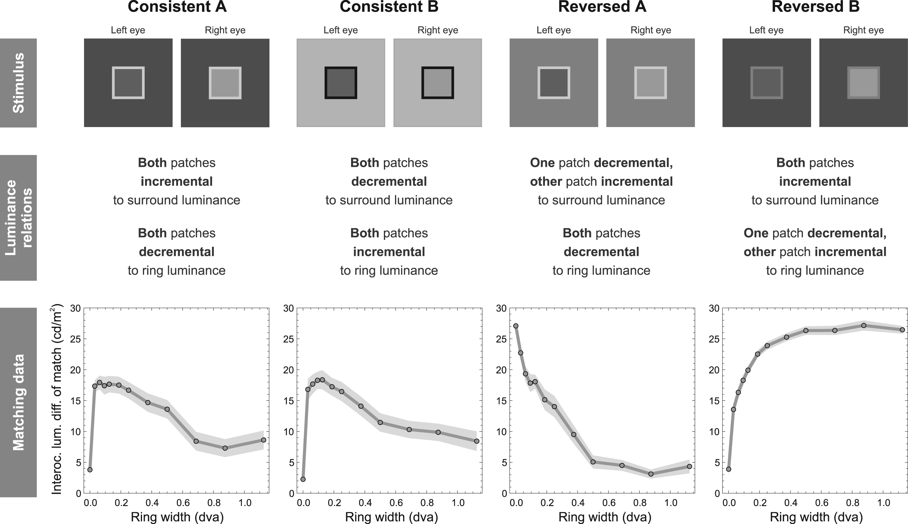
Example results from Wendt and Faul (2025). In a matching experiment, observers had to assess the strength of the lustrous impression in the central area of dichoptic center-ring-surround stimuli with varying ring widths. In addition, four different combinations of ring and surround luminance were tested, which produced different contrast polarity pairings with regard to the center patch luminances (middle row). In the Consistent A and the Consistent B conditions, corresponding contrast polarities always had the same sign in both eyes. In the remaining conditions, either the surround element (Reversed A) or the ring element (Reversed B) produced reversed contrast polarities (inc-dec) between eyes. The strength of the lustrous impression varied strongly depending on the ring width. The shape of the luster curves was determined by the different contrast conditions. The depicted luster settings were obtained with square center patches with a side length of 4 degrees of visual angle and a luminance difference of 30 cd/m2 between the monocular center patches. Transparent areas represent the SEM in both directions.
In our previous work, we have shown that all these observations can be explained by a simple neural process located at an early stage of the visual pathway (Wendt & Faul, 2022a, 2025; see also Appendix A). The basic component of this mechanism is a binocular cell that receives its input signals from two types of monocular contrast detector cells, whose receptive fields have reversed excitatory and inhibitory areas, making them sensitive to light patterns with opposite polarity. Suitable candidates for such monocular cells include neurons with an antagonistic circular-symmetric center-surround organization of their receptive fields (similar to the retinal ganglion ON- and OFF-center cells; see Schiller, 1992), as well as orientation-selective cells, whose excitatory and inhibitory subregions are arranged side-by-side (e.g., with a Gabor-like layout, where the ON- and OFF-cells are represented by opposite phases). One main characteristic of the binocular cell is that its response strongly depends on the types of monocular cells that provide the input signals from corresponding locations of the two eyes. Signals from monocular cells of the same type (ON–ON or OFF–OFF pairings) produce much weaker responses than the pairing of an ON-mechanism with an OFF-mechanism.
The results of adaptation experiments conducted by Kingdom et al. (2018) support the idea that the phenomenon of binocular luster is mediated by specific binocular neurons. Evidence for the existence of binocular cells with the above-mentioned response characteristics has already been provided by Poggio and Fischer (1977). These binocular neurons, located in the primary visual cortex and referred to as tuned-inhibitory cells, have been shown to be highly sensitive to monocular contrast signals with reversed polarity and may serve as a type of interocular conflict detector (Read & Cumming, 2007; see also Goncalves & Welchman, 2017; Katyal et al., 2016; Katyal et al., 2018). Kingdom et al. (2022) therefore assume that these tuned-inhibitory cells may play a crucial role in the luster phenomenon.
Taking the Consistent A and the Reversed B conditions as examples (see Figure 1), we demonstrate in Appendix A how such a mechanism can account for the existing findings (see also Wendt & Faul, 2022a, 2025). These two contrast conditions also play a central role in the present study, as they have some interesting properties: Although they differ only in the luminance of the ring element, this difference has an almost opposite effect on the luster curves. While the lustrous response in the Reversed B condition becomes stronger with increasing ring width, it generally decreases monotonically in the Consistent A condition (after an initial steep increase at very small ring widths, see Figure 1).
In this study, we employed a “hybrid” of these two contrast conditions to investigate how perceived luster depends on more complex stimulus patterns that combine different contrast effects. This can be achieved by dividing the ring into segments that differ either in luminance alone or in both luminance and width (Figure 2). Our study specifically addresses three questions: (1) How are the different influences on the luster phenomenon spatially integrated? For example, do they contribute equally to the overall response (balanced integration) or is the response determined by the stronger of the two effects (winner-takes-all)? (2) Can the luster judgments obtained with such mixed stimuli be predicted by our interocular conflict model, which implements a balanced integration (Wendt & Faul, 2022a, 2025)? Would a circular-symmetric layout of the receptive field of the monocular contrast detector cells lead to different predictions than an orientation-selective side-by-side organization of the excitatory and inhibitory regions? (3) Finally, is the lustrous impression within the target area of these mixed stimuli spatially homogeneous, and if not, how does the perceived inhomogeneity affect the overall luster judgments?
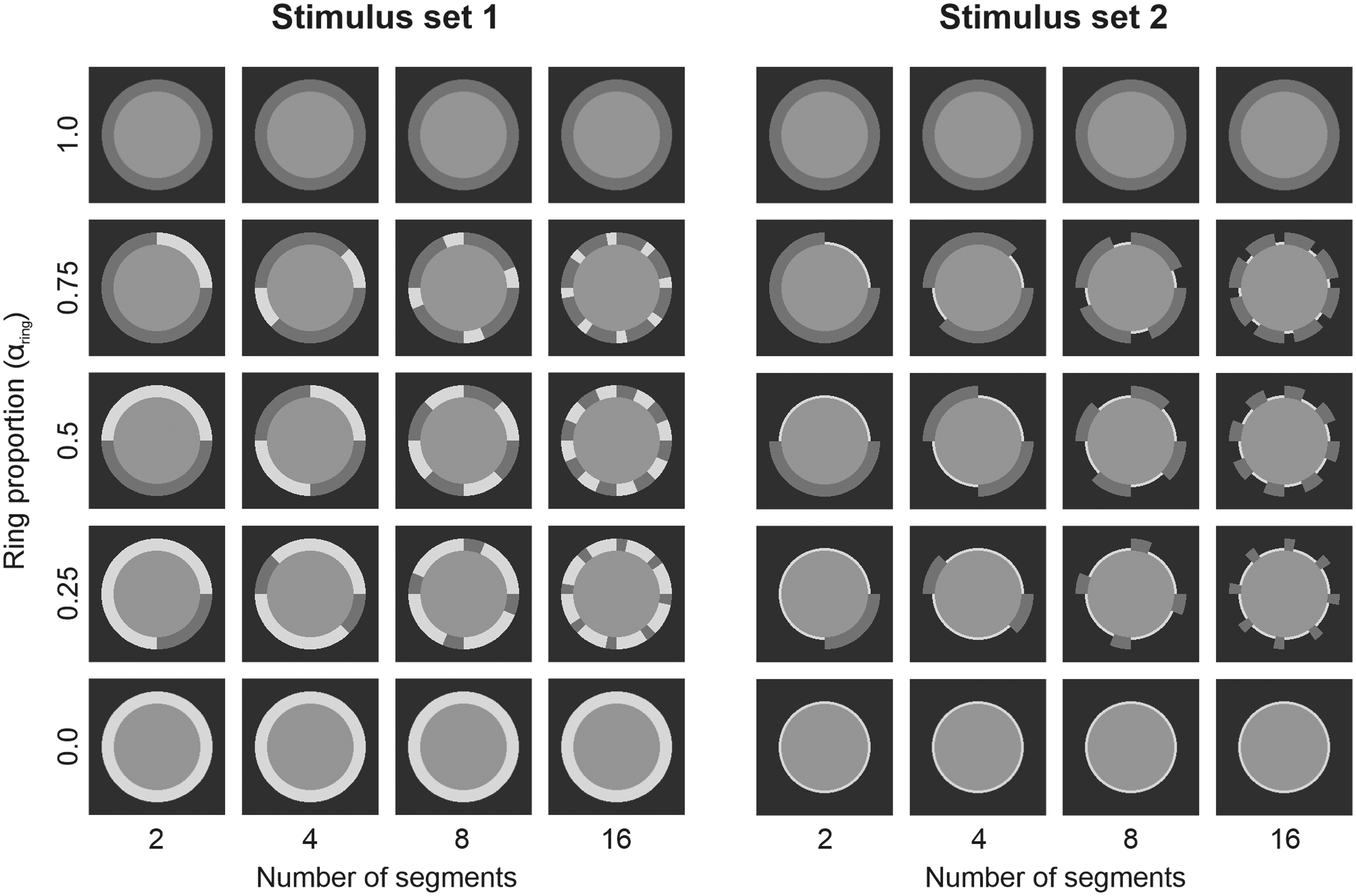
Ring structures as they were used in the two different stimulus sets. In set 1 (left panel), the two ring parts generally had different luminances (except for stimuli with ring proportions of 0.0 or 1.0, respectively) but the same ring width in each stimulus (here shown with a fixed ring width of 0.5625 dva). In set 2 (right panel), one ring part had a constant width of 0.5625 dva and a luminance of 25 cd/m2, whereas the other ring part had a variable width and a luminance of 75 cd/m2 (here shown with a constant ring width of 0.125 dva).
Methods
Observers
Eight subjects participated in the experiment, one of them being the first author of the study (GW). Five of the participants were female and three male, with their ages ranging from 20 to 53 years. All subjects had normal or corrected-to-normal visual acuity. Prior to the experiment, we obtained written informed consent from all subjects. The study was conducted in agreement with the ethical standards of the Deutsche Forschungsgemeinschaft (German Research Foundation, DFG) and was approved by the Central Ethics Committee of Kiel University (ZEK-18/24).
Stimuli and Apparatus
In order to test how the visual system spatially integrates different contrast effects on binocular luster, we used dichoptic center-ring-surround configurations with a circular shape as test stimuli that were mixed versions of the two original contrast conditions Consistent A and Reversed B (see Figure 1; note that we use the term contrast effects in a largely descriptive sense here to refer to the different effects on the lustrous response produced by the two “pure” contrast conditions Consistent A and Reversed B). We used stimuli in which the ring element was subdivided into either 2, 4, 8, or 16 segments, where neighboring segments either differed in luminance only (stimulus set 1, left panel in Figure 2), or both in luminance and width (stimulus set 2, right panel in Figure 2). In addition, we varied the relative length of the two segment types. The ring proportions are defined by the mixing factor αring, which represents the relative length of the stronger ring part (based on the Reversed B contrast condition, see Figure 1), whereas the weaker part (based on the Consistent A condition) has a proportion of 1.0 - αring. Stimuli with αring = 0, 0.25, 0.5, 0.75, and 1.0 were tested. Stimuli with αring = 0 and 1.0 are the two original contrast conditions with a uniform ring. Finally, we varied the width of the ring segments, either equally for the two ring parts (stimulus set 1), or for one ring part only, while the other ring part was kept at a constant width (stimulus set 2). Ring widths of 0.0, 0.0625, 0.125, 0.25, 0.375, 0.5625, 0.8125, and 1.0625 dva were used for the varying part of the ring in stimulus set 2. In stimulus set 1, however, the no-ring condition (0 dva) was omitted, because this condition would produce identical center-surround stimuli for all combinations of segment number and ring proportion. The luminance of the common surround, which covered the entire upper half of the monitor in which the test stimuli were presented, always had a constant luminance of 5 cd/m2. The circular center patches, representing the target area of the stimuli, had a radius of 2.0 dva and a luminance of 10 cd/m2 for one eye and 40 cd/m2 for the other (these luminances were swapped between eyes in half of the trials to account for potential imbalances in eye dominance).
The stimuli were displayed on a monitor with a diagonal of 24 inches (EIZO CG243 W) and a resolution of 1,920 × 1,200 pixels. To color calibrate the monitor, a JETI specbos 1211 spectroradiometer was used, following a method described in Brainard (1989). The dichoptic stimulus pairs were presented side by side on the screen and fused using a mirror-stereoscope (ScreenScope) mounted on the monitor. The light paths from the screen to the observer's eyes had a length of 50 cm.
Procedure
In each trial, observers evaluated three properties of the test stimulus. First, they had to determine whether the target area of the test stimulus appeared lustrous at all. To this end, the test stimulus (in the top half of the monitor) was presented together with an anchor stimulus (in the bottom half). While the ring structure and the background of the anchor stimulus were always identical to those of the test, the center patches of the anchor always had the same luminance of 22.5 cd/m2 and thus appeared matte. This luminance was chosen such that (a) it was close to the mean luminance of the two center patches of the test stimulus (which was always 25 cd/m2) and (b) it still allowed for spatial discrimination between the center patch area and the ring area in cases where the ring element had a luminance of 25 cd/m2. This anchor stimulus was meant to facilitate the detection of weaker lustrous sensations in the test. Using the arrow keys on the keyboard, the observer could switch between the two response alternatives “lustrous” and “nonlustrous.” If “nonlustrous” was selected, the trial was terminated and the next trial began after a dark adaptation period of 3 s. If “lustrous” was selected, the trial proceeded to the second part, in which the test stimulus was presented together with a matching stimulus consisting of a dichoptic center-ring-surround configuration with a square outline (Figure 3). The center patches of the match had a side-length of 2.0 dva and were enclosed by a 0.125 dva wide ring with a fixed luminance of 25 cd/m2. The luminance of the common surround, which filled the entire bottom half of the screen, was 10 cd/m2. Using the arrow keys on the keyboard, the observer had to adjust the interocular luminance difference |Cl – Cr| between the two center patches such that the perceived luster in the match was indistinguishable from that of the target patch of the test stimulus. This luminance difference was used as a measure for the perceived luster strength (see also Wendt & Faul, 2025). This choice is supported by the strong correlations between the interocular luminance difference |Cl – Cr| and corresponding rating values in our previous studies (Wendt & Faul, 2020, 2022a, 2024), in which the observers additionally rated the strength of the lustrous impression on a scale from 0 to 5. The observers adjusted a parameter p, which was used to determine the two luminances, Cl and Cr, of the centers of the match as follows:
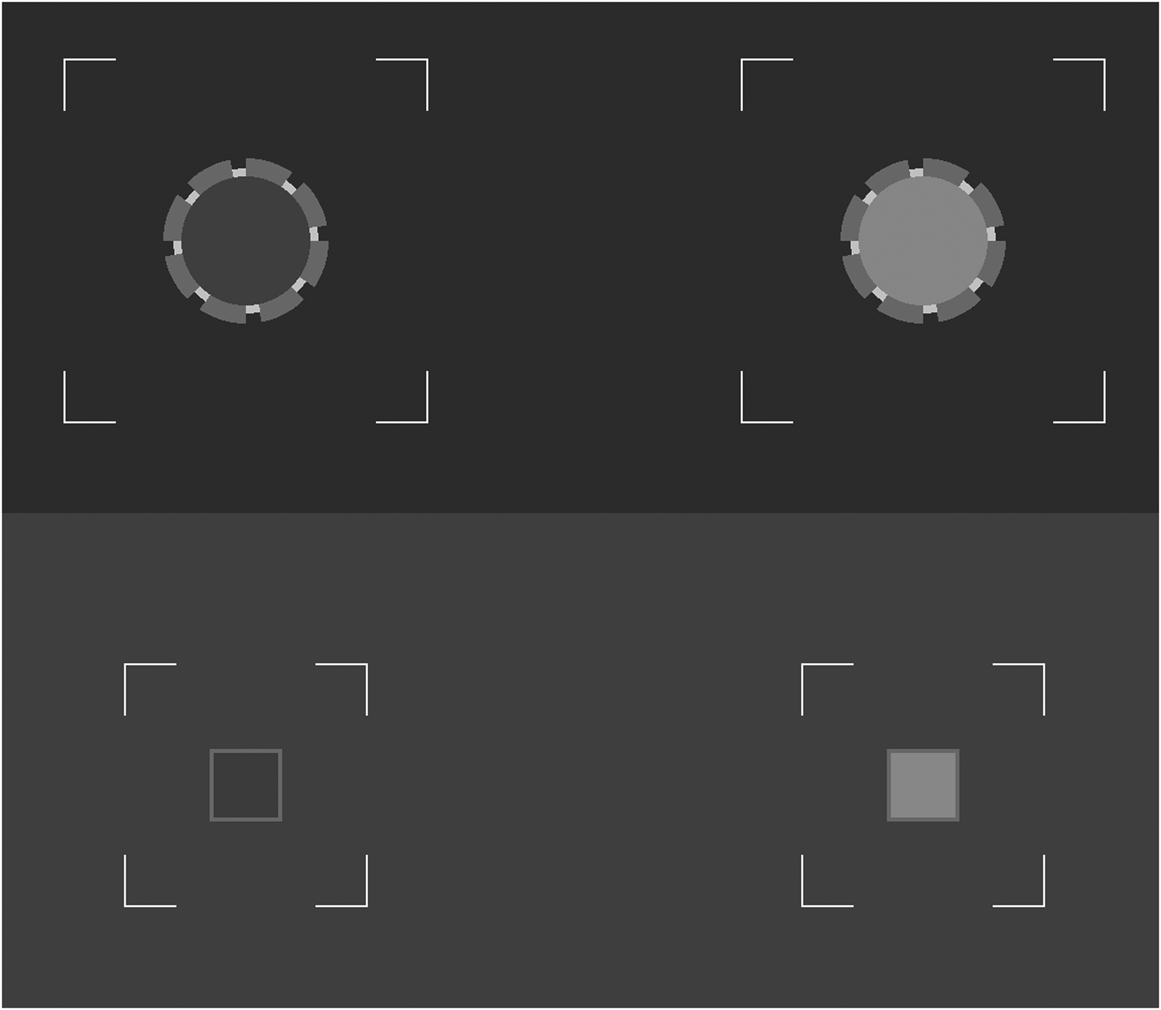
Central part of the screen area during the matching task. The dichoptic test stimulus was always presented in the upper half of the screen, the matching stimulus always in the lower half. The task of the subject was to adjust the interocular luminance difference between the two center patches of the match such that the perceived luster was indistinguishable from that of the test stimulus.
Cl,r = 25 · (1 ± ps) cd/m2, for 0 ≤ p ≤ 1 and s = 1/0.77.
The constant s in this equation was selected such that the relationship between p and the strength of perceived luster was approximately linear (see Wendt & Faul, 2019).
Since the two different ring parts of the mixed-ring stimuli have different effects on the lustrous impression, it is possible that the perceived strength of the luster varies spatially within the target patch. For instance, areas close to the ring parts with the stronger effect could be perceived as more lustrous than areas adjacent to the weaker ring parts. This could be problematic for the matching task, as the observer has to match the perceived luster in the test with a match stimulus that always produces a uniform lustrous appearance. In these cases, a perfect match would be difficult to achieve and the observer may then use an alternative (conscious or unconscious) strategy to complete this task, for instance, by basing the luster judgment exclusively on those areas with the stronger luster or by using a weighted mixture. To check whether such effects could play a role in our study, we asked the observers in the third part of a trial to assess the perceived spatial homogeneity of the luster within the target area. To this end, the same test stimulus as in the previous two parts of the trial was shown in isolation and the observer had to select an integer rating value between 0 (= “extremely inhomogeneous”) and 10 (= “perfectly homogeneous”) using the arrow keys on the keyboard.
Prior to the experiment, each observer was carefully instructed and a series of test trials had to be performed under the supervision of the experimenter. The stimuli used in these test trials were selected from the entire set of stimulus conditions used in the experiment and provided a wide range of different luster impressions. In total, 210 different stimulus combinations were tested, each of them with four repetitions. The entire set of trials was presented in random order.
Calculating the Predictions for the Mixed-Ring Conditions
The empirical luster curves were evaluated with respect to two alternative integration mechanisms: a winner-takes-all integration and a balanced integration.
Winner-Takes-All
Under a winner-takes-all integration model, the magnitudes of the lustrous responses obtained with the mixed-ring stimuli (combining a stronger and a weaker effect) should equal those of the “pure” condition with the stronger effect. That is, in combinations of the stronger Reversed B condition and the weaker Consistent A condition, a winner-takes-all mechanism would produce the same lustrous response as Reversed B stimuli with a homogeneous ring (with αring = 1.0, see Figure 2). Therefore, the luster curves associated with the mixed-ring stimuli should then be identical to the curve observed with the stronger effect in the pure condition.
Balanced Integration
In a balanced integration model, different predictions for the lustrous responses obtained with the mixed-ring stimuli can be derived. We tested two alternatives:
A very intuitive method is to predict these luster curves on the basis of the two pure luster curves with uniform rings. It would be reasonable to assume that the luster curve for the mixed-ring stimuli results from a weighted combination of these two curves, with the weights corresponding to the respective ring proportions. That is, with a fixed proportion of αring it would be a convex combination of the luster curve for the stronger effect weighted by αring and the luster curve for the weaker effect weighted by 1.0 - αring. As an alternative to this descriptive or combined-data method for predicting the luster curves, we applied a method based on our interocular conflict model of binocular luster (Wendt & Faul, 2022a; a detailed description of the model is provided in Appendix A). Since this model incorporates a balanced integration of the conflict signals within the target area, it seems well suited for predicting the luster curves for the mixed-ring conditions. The model was fed with the same stimuli used in the experiment to predict the corresponding empirical luster curves for the mixed-ring stimuli. The model parameters required for calculating these predictions were estimated using the empirical data obtained under the two pure contrast conditions Consistent A and Reversed B. Furthermore, as mentioned in the Introduction, we used two different variants of the model for the predictions, which differ in the type of filter kernel that represents the monocular contrast detector cells. The receptive field has either a circular-symmetric center-surround organization, which was simulated with a Laplacian of Gaussian filter kernel (LoG, see Appendix A), or a side-by-side arrangement of the excitatory and inhibitory areas simulated with Gabor filters (see Appendix B). There is evidence from neurophysiological studies for the existence of both cell types in the primary visual cortex (Hubel & Wiesel, 1962; Sincich & Blasdel, 2001), making both suitable candidates for representing the monocular level in our model. The comparison between these two types of filter kernels was also motivated by the fact that mixed-ring stimuli often show a complex pattern of luminance edges that occur not only between the target area and the ring element but also between neighboring ring segments (which produce so-called T-junctions with luminance edges that are orthogonal to each other, see Figure 2). This suggests that an orientation-selective filter kernel may lead to different predictions than a filter kernel based on an LoG kernel—and, if true, this may provide some deeper insights into the specific types of monocular contrast detector cells involved in the underlying mechanism. Since both models are based on the between-eye interaction of ON and OFF contrast mechanisms, we will refer to the two variants in the following as the LoG ON–OFF model and the oriented ON–OFF model, respectively.
Results
Since all mixed-ring stimuli combine the pure contrast conditions Consistent A and Reversed B, we will first take a look at the luster curves for these basic stimulus sets. The luster settings averaged across all eight subjects are shown in the top row of Figure 4 as colored symbols (left diagram, yellow for the Consistent A and blue for the Reversed B condition). Also shown are the corresponding predictions and best-fitting parameter values of the LoG (middle diagram, see also Appendix A) and the oriented ON–OFF model (right diagram, see also Appendix B). The luster curve for the Reversed B condition (blue) is very similar to those observed in our previous studies (see Figure 1). The curve for the Consistent A condition, however, deviates considerably from previous results. The general shape of the curve is similar: it is non-monotonic with a steep increase between the no-ring condition and a ring width of 0.0625 dva, and a smoother decrease at larger ring widths. However, the peak of the curve is shifted to a much larger ring width (at 0.375 dva) and the decrease of the luster settings for subsequent ring widths is much smoother than we previously found.
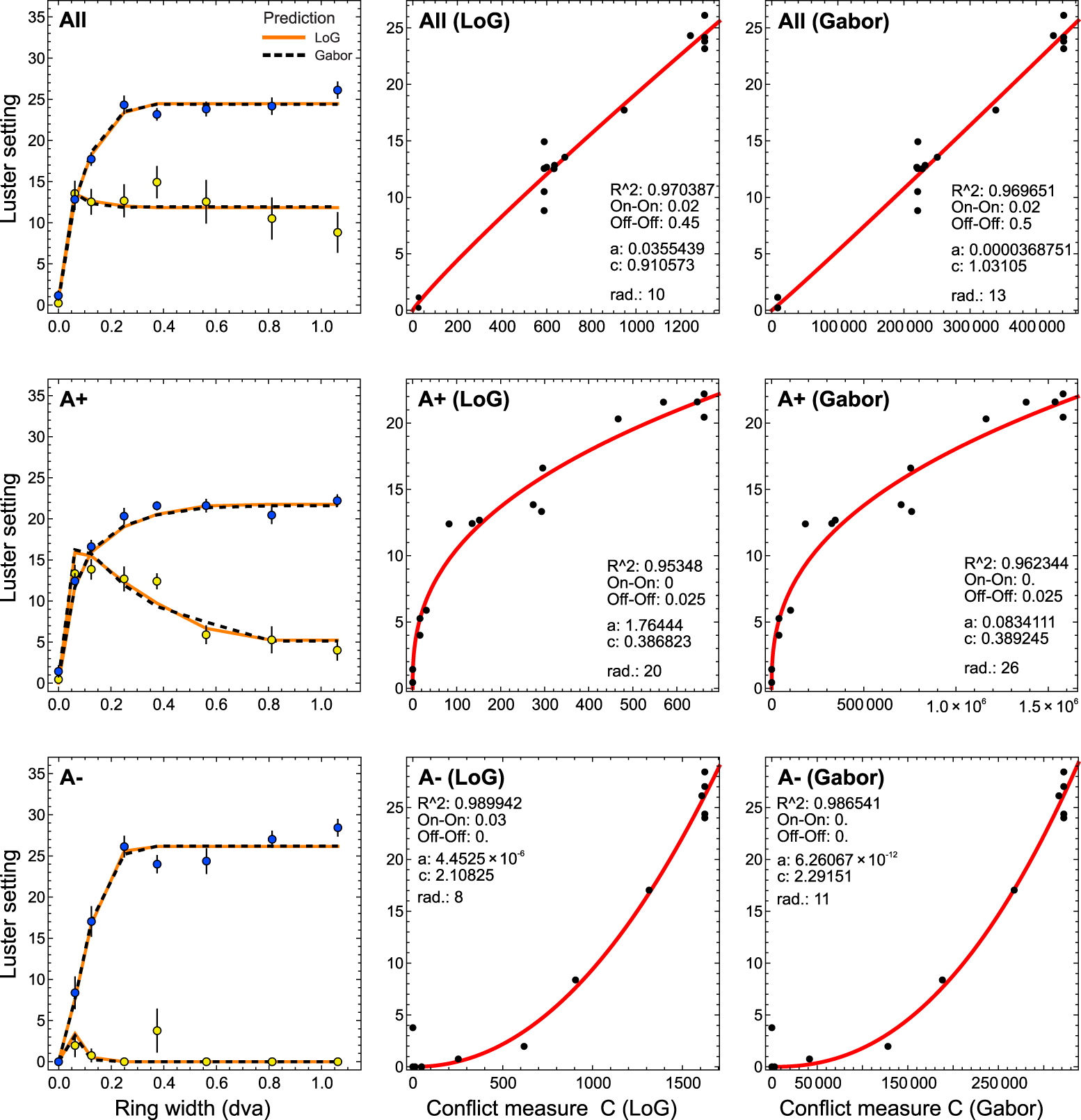
Left column: empirical luster settings for the pure Consistent A (yellow disks, error bars represent the SEM in both directions) and Reversed B (blue disks) contrast conditions and their corresponding predictions based on the LoG (orange lines) and the oriented ON–OFF model (dashed black lines). The middle and the right diagrams show the relationship between the empirical luster settings and the conflict measure C for the LoG (middle diagram) and the oriented ON–OFF model (right diagram), respectively, based on the parameters of the best fit. Note that conflict measure C is not the final output of the model (which is C’, as it was used for the prediction lines in the left diagrams, s. also Appendix A), but an intermediate result which we use here to demonstrate the shape of the transducer functions (red curves). The top row shows the results for the entire sample of eight subjects, the middle and bottom rows those for the two sub-groups
The reason for this unexpected shape of the Consistent A luster curve becomes clearer when comparing the empirical luster settings of the individual subjects (see Appendix C). In the Reversed B condition, the luster curves of all subjects have a similar shape: The lustrous response increases sharply with increasing ring width until it reaches an asymptote, with slight variations in the steepness of the increase and the absolute level of the asymptote. However, the subjects show clear differences in their sensitivity to luster in the Consistent A condition. There appear to be two main trends, which are also reflected in the parameter values of the corresponding model fits. One group of subjects (S01, S02, and S04), who showed high luster sensitivity for stimuli from the Consistent A condition (which we will refer to as the
Figures 5 and 6 show the empirical results of the matching task for the
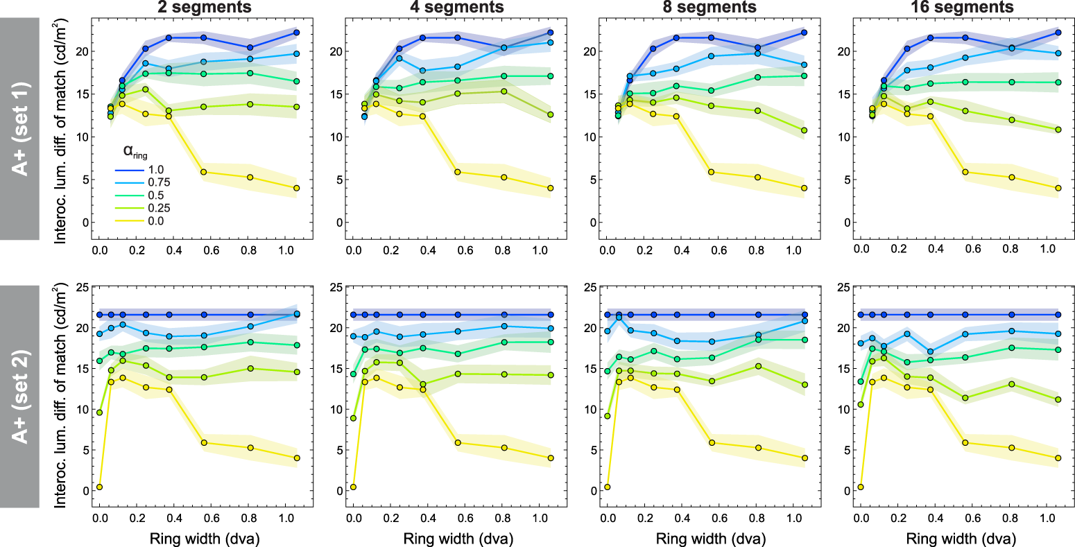
Results of the matching task of group
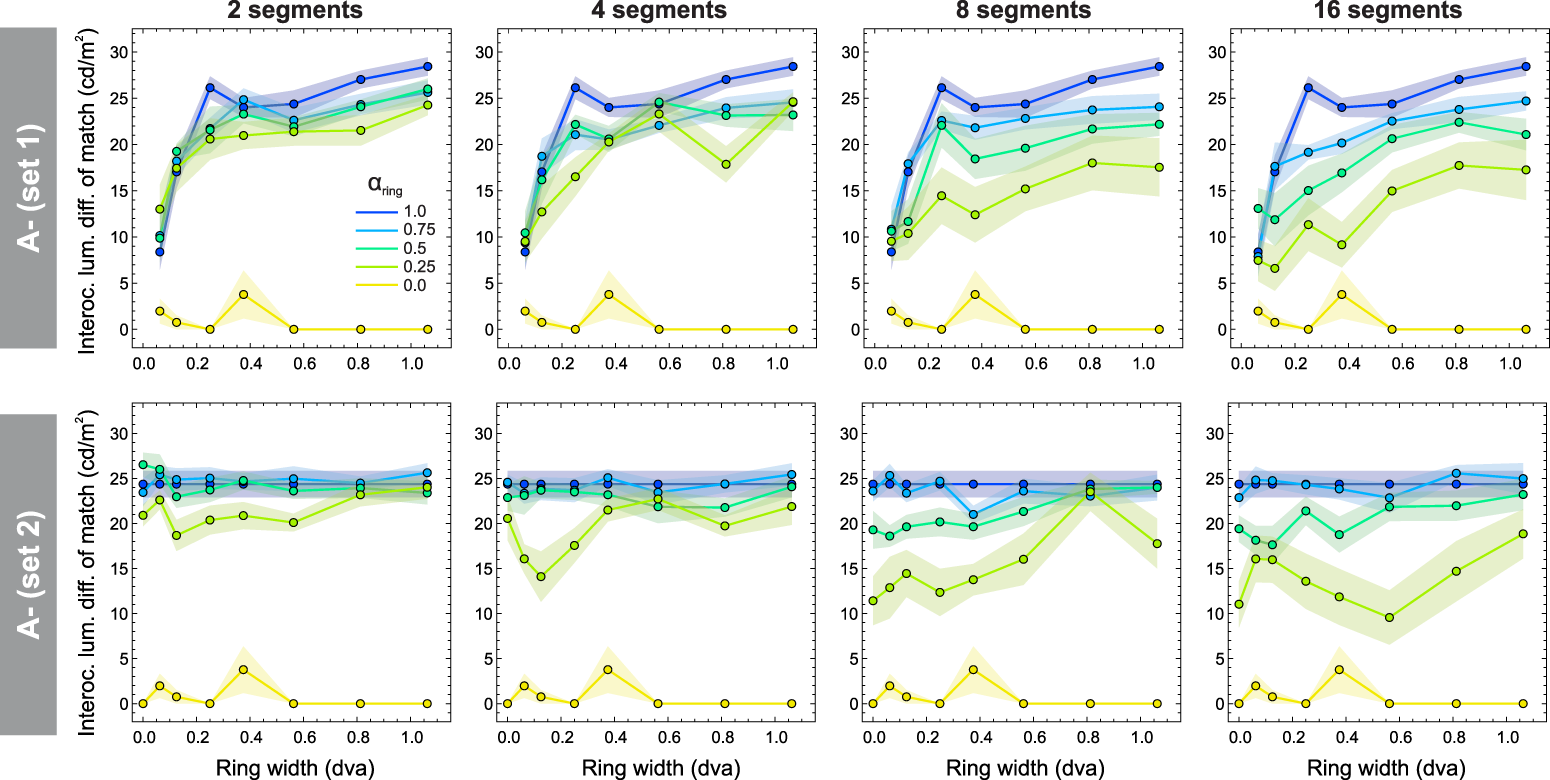
Results of the matching task of group
We will now compare the findings of both groups, starting with the results of the
So far, it is obvious that the data cannot be explained by the assumption that the stronger of the two contrast effects fully determines the lustrous appearance in the mixed-ring stimuli (winner-takes-all). But how well are the empirical luster curves predicted by the alternative integration process, which assumes equal weights for the two effects? In Figure 7, we give a first impression of how the data of the two different subject groups
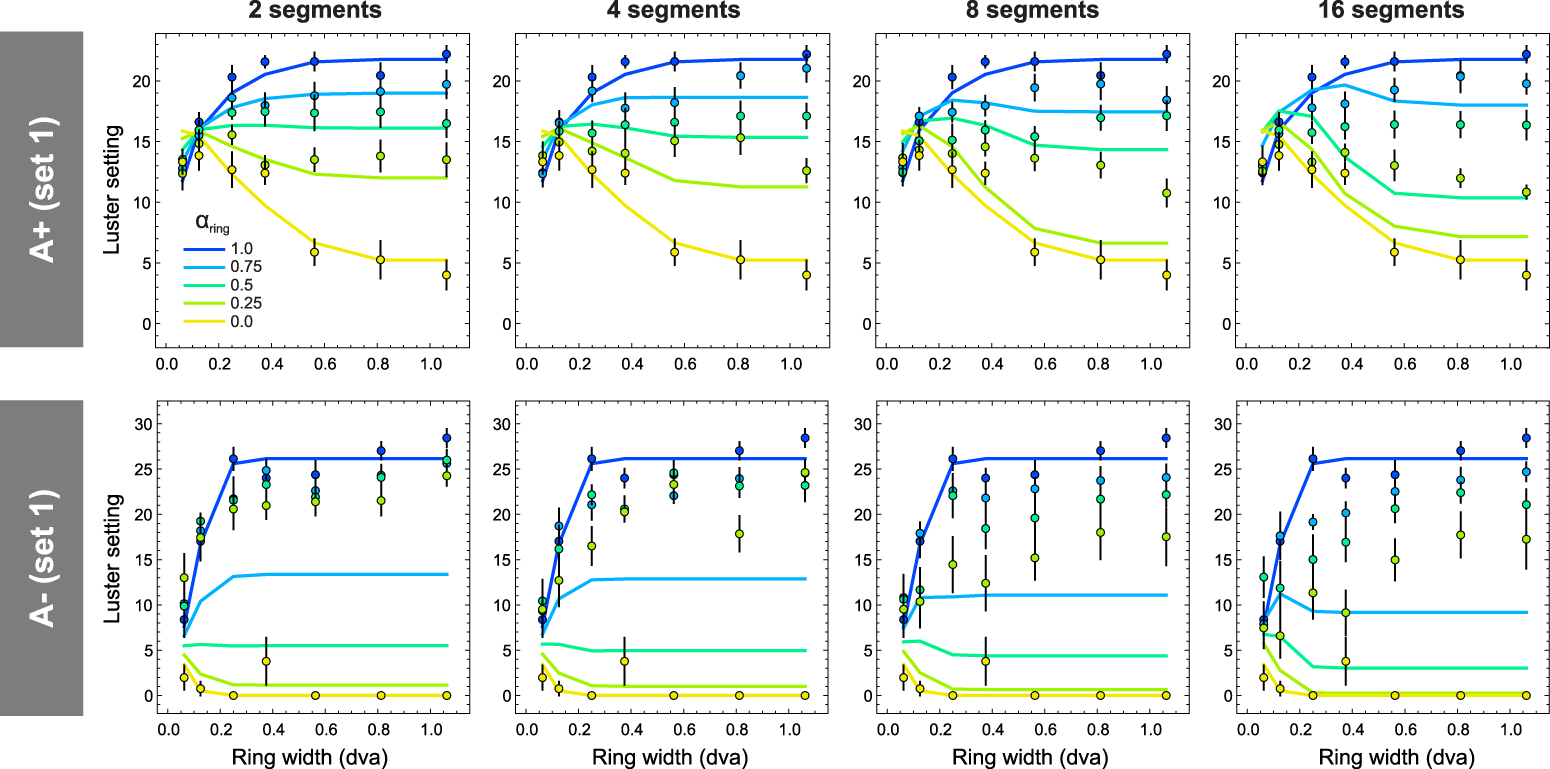
Example luster settings (colored disks) obtained with stimulus set 1 for groups
To provide a more condensed overview of how the empirical luster data relate to the corresponding predictions for the two alternative integration methods, we calculated an index k that indicates how strongly each luster curve deviates from its prediction for balanced integration, relative to the prediction for the winner-takes-all integration. This means that index k lies in an interval between 0.0 and 1.0, where a value of 0.0 means that the given luster curve is fully consistent with the assumption of balanced integration, whereas a value of 1.0 means that the data perfectly align with a winner-takes-all integration process. Values between these poles mean that the two different contrast effects are integrated by an “unbalanced” mechanism, in which the stronger contrast effect has a greater weight than the weaker effect, that is, the higher the index k, the greater the weight for the stronger contrast effect.
For the combined-data method, in which each prediction curve is a convex mixture of the two pure luster curves with a spatially uniform ring (the blue and the yellow curves in the respective diagrams, see Section 2.4), we determined the mixing factor αemp that best fits the empirical luster curve. We then set αemp in relation to the two values representing the two different integration methods, where αbal represents balanced integration (which is identical to the spatial proportion αring of the mixed-ring stimuli) and αwin = 1.0 represents winner-takes-all integration (see the left diagram in Figure 8): kdata = (αemp – αbal) / (1.0 – αbal).
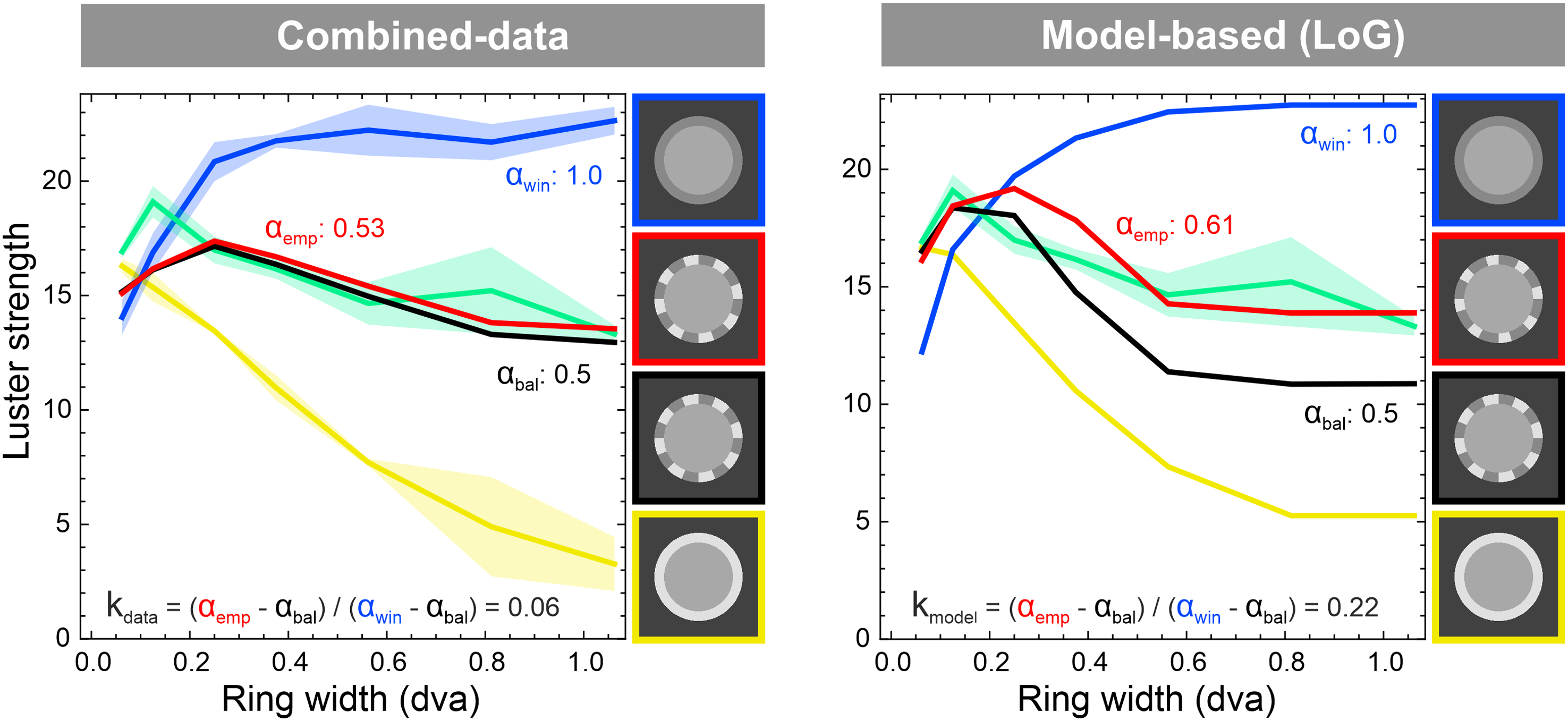
Illustration of how the indices kdata (left) and kmodel (right) are calculated. As an example, we use the luster curve from subject S01 of the first stimulus set where the mixed-ring condition had 16 segments and a spatial proportion of αring = 0.5 (stimulus with black frame). For the combined-data method, the empirical luster curve (green) was fitted with a convex combination of the two curves that represent the pure effects (yellow for the weaker effect, blue for the stronger effect). For the model-based method, the parameter αemp represents the spatial proportion of that specific stimulus (with varying ring widths), for which the model calculates a curve (red) that best fits the empirical luster curve (green). In both cases, index k represents how strongly the empirical luster curve deviates from the curve representing the prediction for the balanced integration method (αbal, black), relative to the prediction for the winner-takes-all integration method (αwin, blue, which always has a value of 1.0): k = (αemp − αbal) / (1.0 – αbal).
For the model-based methods, we had to a use a different approach to determine the best fit for the empirical luster curve, as this method requires actual stimuli to calculate a model output (see Appendix A). We therefore needed additional stimuli in addition to those used in the experiment: For each segment number and each ring width, we generated mixed-ring stimuli with spatial proportions αi for the two ring parts between 0.0 and 1.0 in steps of 0.01 leading in each case to 101 candidate curves. We then determined for each empirical luster curve, which of the 101 curves best fits the empirical curve and set αemp to the corresponding αi and calculated the index kmodel in the same way as kdata (see the right diagram in Figure 8).
Figure 9 shows the different types of k indices (columns) separately for the two groups
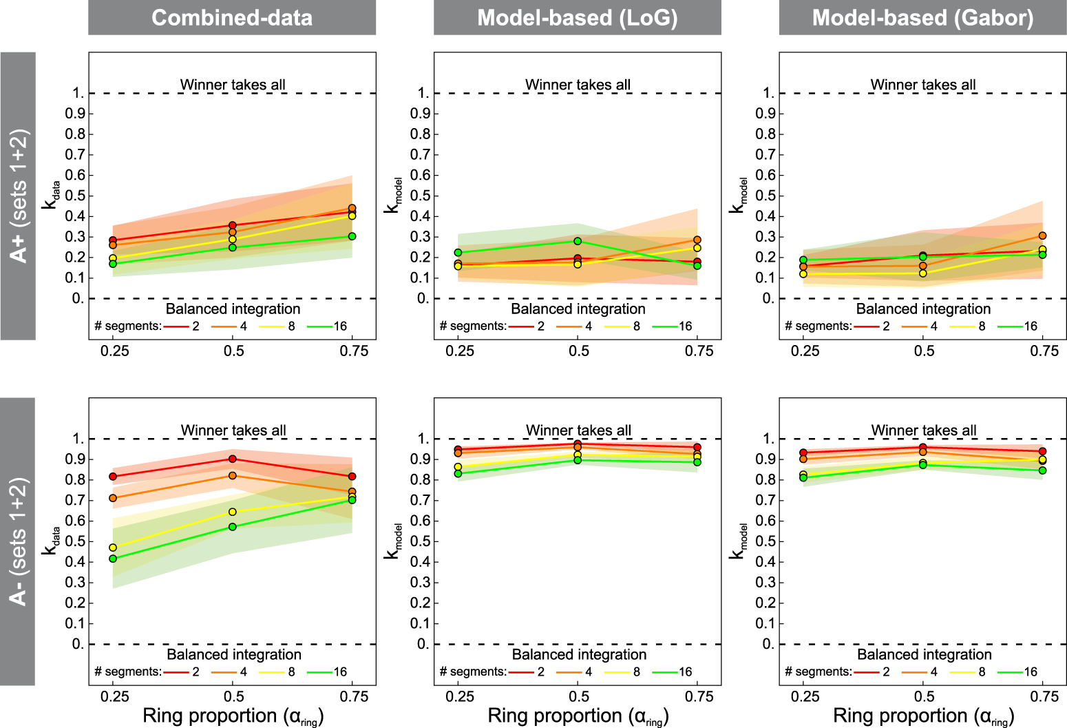
The different types of k indices calculated using either the combined-data method (left column) or the model-based method (middle column for the LoG, right column for the oriented ON–OFF model), separately for the two subject groups
Figure 10 shows the results of the homogeneity rating task, separately for the two groups
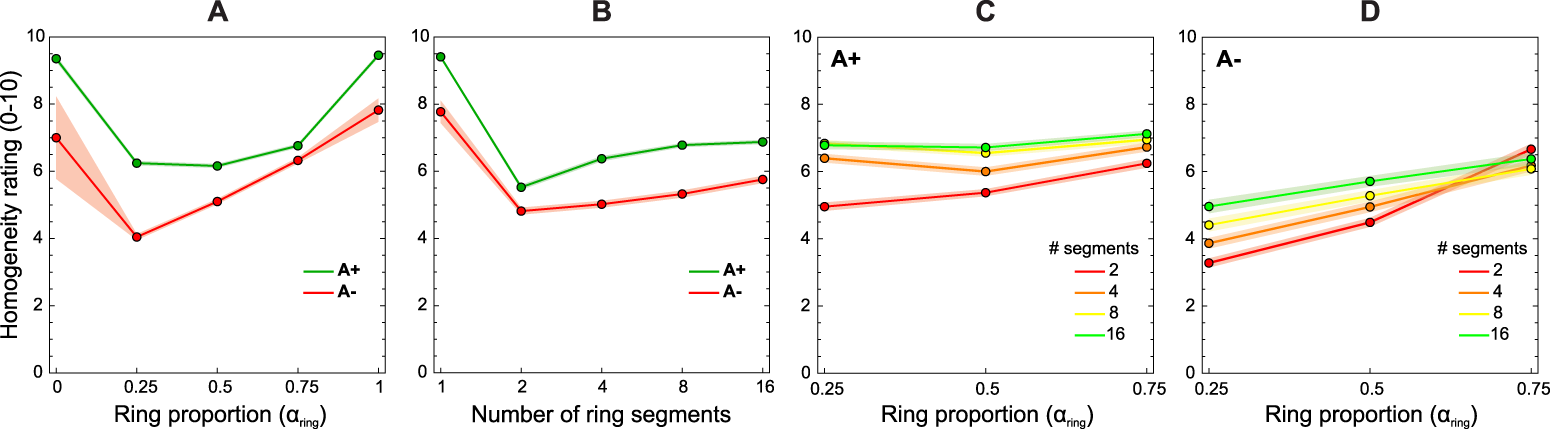
Results of the homogeneity rating task. Diagrams A and B show the mean homogeneity ratings depending on the spatial proportion between the two ring parts (A) and the number of ring segments (B), separately for the two groups
Panels A and B in Figure 10 reveal two very clear trends. First, both groups perceived the luster in the target area of the mixed-ring stimuli (with spatial proportions between 0.25 and 0.75 or segment numbers greater than 1, respectively) as significantly less homogeneous than in the two pure conditions with a full ring. Second, spatial homogeneity of the lustrous impression was generally rated significantly lower by group
Discussion
The results of the matching task suggest that the two subject groups
To test the assumption of a balanced integration, we used different methods to calculate corresponding luster predictions for the mixed-ring stimuli (see Appendix D), namely a combined-data method and two model-based methods, which are based on the LoG ON–OFF model and the oriented ON–OFF model variant, respectively (see Section 2.4.). To determine how well the empirical luster data obtained with the mixed-ring stimuli could be predicted by the two model-based methods, we calculated the corresponding prediction curves using the same model parameters that had previously been determined by fitting the data of the two pure contrast conditions Consistent A and Reversed B (see Figure 4), separately for the two subject groups
However, if these models (including the combined-data method) are applied to the mixed-ring data, none of them is able to accurately predict the empirical luster settings. The best results, in terms of the coefficient of determination R2, were obtained for group
The failure to predict the mixed-ring data with these models (which assume balanced integration) therefore suggests an unbalanced integration of the two contrast effects, where both effects contribute to the lustrous impression, but with different weights. In both groups, the stronger of the two contrast effects has a higher weight than the weaker one; however, this weighting asymmetry is considerably more pronounced for group
It is worth noting that the two parametric models (i.e., the LoG ON–OFF model and the oriented ON–OFF model) provide significantly better predictions if we include the data obtained under the two pure contrast conditions and then redetermine the best-fitting model parameters based on these complete datasets for the two subject groups. The goodness of fit is very similar for the two model variants; however, as before, the predictions for group
We next investigate why the kdata and the kmodel indices differ. By construction, the combined-data method produces luster curves that are equally spaced and do not depend on the number of ring segments (see the lines in the top panels of Figures D1 and D2 in Appendix D). In contrast, the model-based predictions show shifts that are not only influenced by the number of ring segments but also clearly differ between groups
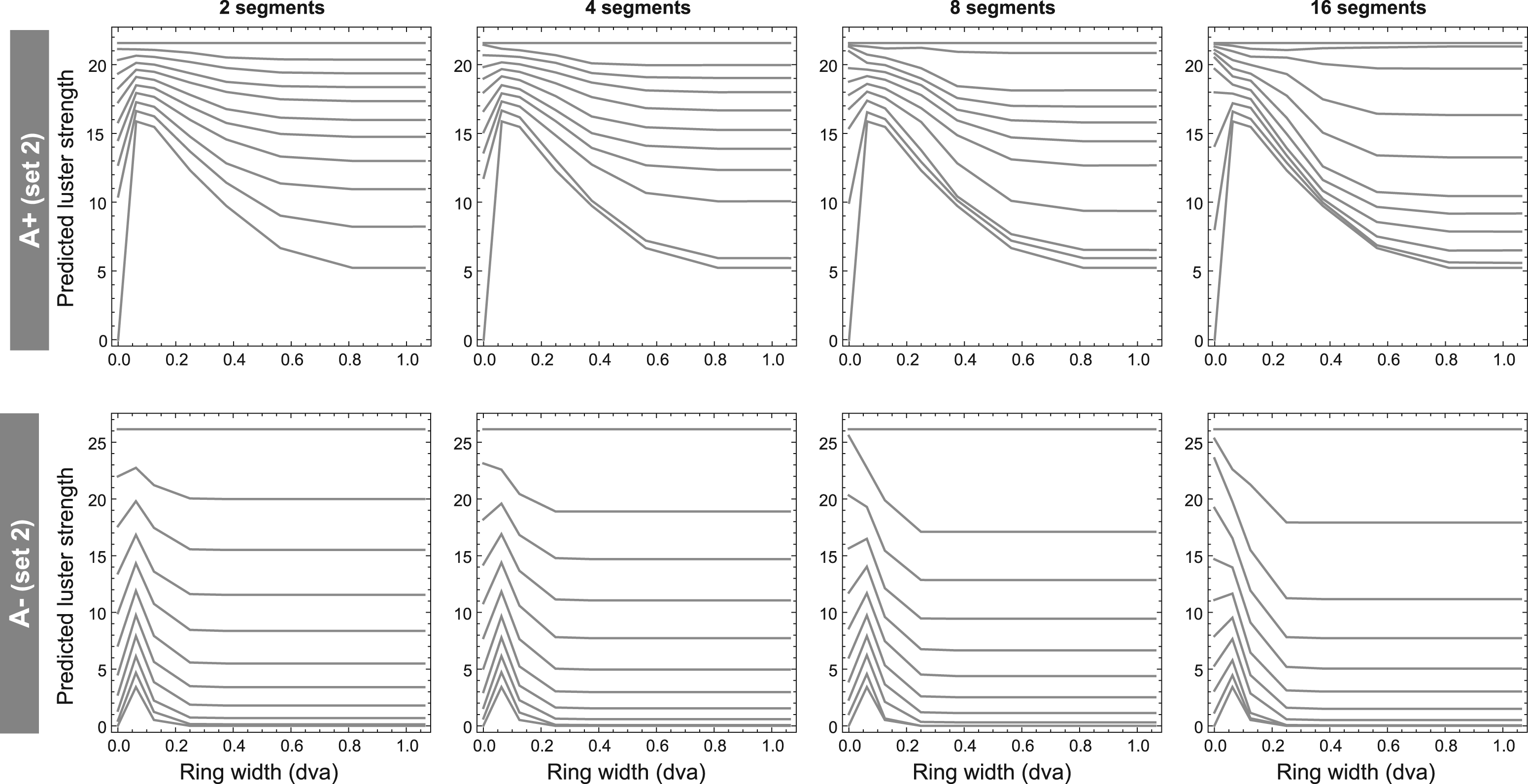
Curve shifts in the model-based predictions. The diagrams show the predicted luster curves for stimuli of set 2 based on the LoG ON–OFF model for eleven different ring proportions (between 0.0 and 1.0 in steps of 0.1) and the four different segment numbers (columns), separately for group
The first effect is most clearly observed in the diagrams showing the prediction curves for stimuli with only two ring segments, because these curves are only weakly affected by the second effect, which depends on the number of ring segments (left column in Figure 11). For group
The second effect underlying the shifts of the luster curves strongly depends on the number of ring segments and has its origin at the level of the monocular contrast detectors, which in our model are simulated either with an LoG or a Garbor filter kernel. As shown in Figure 11, with increasing number of ring segments the luster curves tend to move downward. That is, the more ring segments, the weaker the lustrous impression becomes—an effect that has the same direction for both subject groups. As mentioned in the model description (Appendix A), the magnitude of the lustrous response mainly depends on the relative proportion of local conflicts produced by ON–OFF pairings, whereas ON–ON and OFF–OFF pairings contribute much less to the overall response (Figure A2 in Appendix A). Figure 12 illustrates how the proportion of these ON–OFF pairings depends on the number of ring segments, using example stimuli from stimulus set 1. Figure 12A illustrates which types of monocular contrast mechanisms are activated at different locations within the target area of the stimulus. OFF-center mechanisms are stimulated at corresponding positions when the filter kernels exclusively cover areas that include the lighter ring part (associated with the weaker Consistent A condition, see the red areas in Figure 12). Stronger ON–OFF signals are generated at those locations, at which the filter kernels cover areas that only contain the darker ring part (associated with the Reversed B condition, see the yellow areas in Figure 12). The critical stimulus locations responsible for the reduction of ON–OFF signals are intersections between the two different ring parts where two different ring luminances are spatially integrated by the filter kernels. In these cases, slightly less ON–OFF pairings than pairings with equal polarities are produced. For the stimulus example with two ring segments shown in Figure 12A, the proportion of ON–OFF pairings is about 48%. With increasing number of ring segments, and therefore with increasing number of such intersections, the relative number of ON–OFF pairings continuously decreases until it reaches a proportion of less than 36% with rings having 16 segments (Figure 12B). Note that this effect also depends on the size of the filter kernel. At some locations within the target area, larger kernels can even cover more than two ring segments. This is especially the case for group
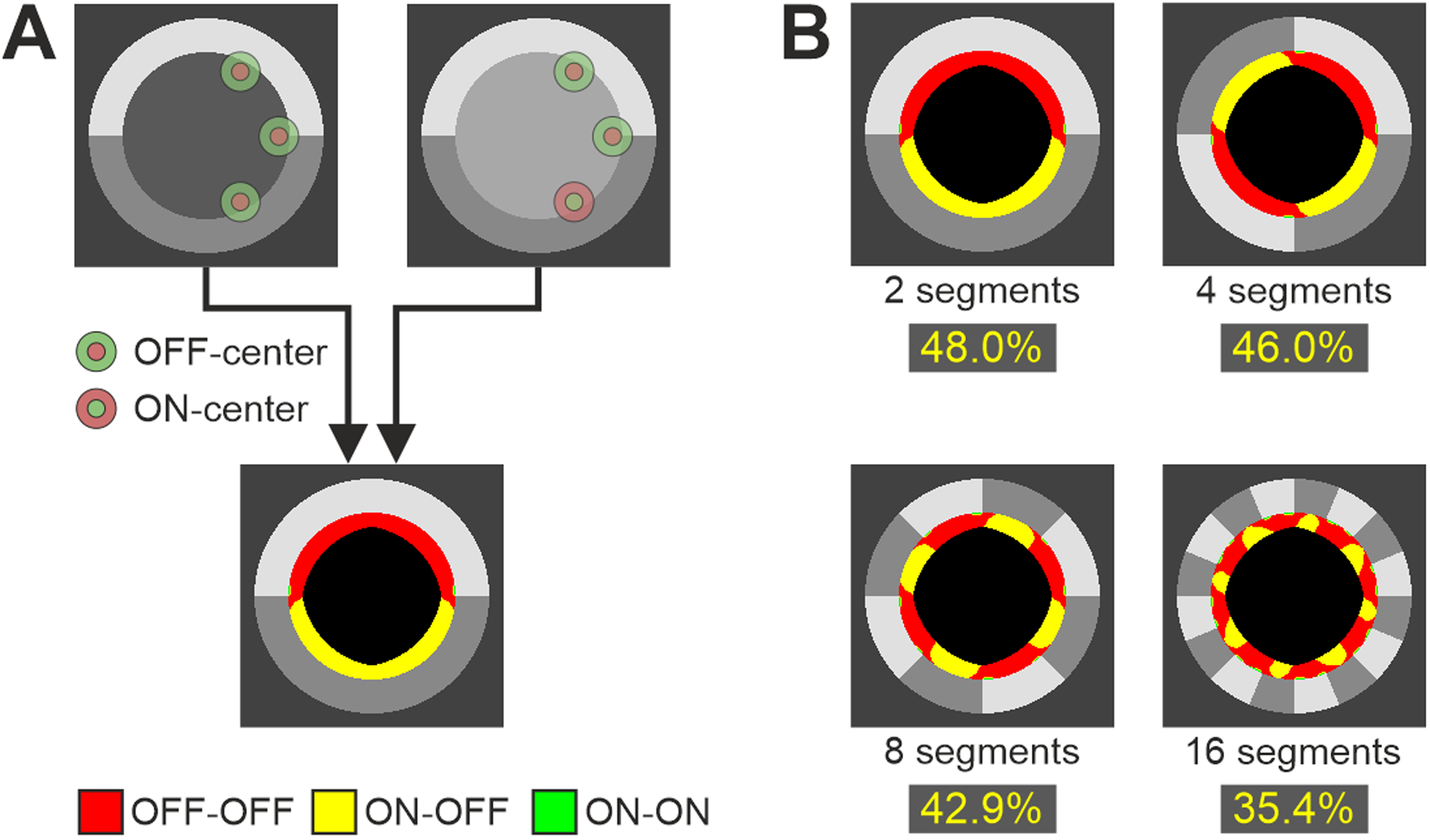
Why do the model-based predictions depend on the number of ring segments? (A) Example stimulus pair from the first stimulus set with a ring subdivided into two segments. Filter kernels that exclusively cover one ring part either produce weak OFF–OFF pairings (red areas) or strong ON–OFF pairings (yellow areas). At the intersections between two ring parts, at which two different ring luminances are spatially integrated by the filter kernel, more OFF–OFF than ON–OFF pairings are produced. (B) The proportion of ON–OFF signals continuously decreases with increasing number of ring segments, or number of intersections, respectively. Since the magnitude of the model output mainly depends on the number of strong ON–OFF signals, this explains why the model predicts weaker lustrous responses for stimuli with increasing number of ring segments.
The differences between the kdata and the kmodel indices are therefore due to the fact the model-based method predicts curve shifts that depend on both the number of ring segments and the different sensitivities to the luster phenomenon, whereas the combined-data method does not take either of these influences into account. At least with regard to the number of ring segments, the empirical data indicate that the magnitude of the lustrous response does indeed depend on this variable. In particular, the results of group
However, an alternative interpretation for this effect exists that is not based on the properties of our model. The results of the homogeneity task suggest that the number of ring segments also has an influence on the spatial homogeneity of the luster (Figure 10). As the number of segments increases, the luster within the target area is increasingly perceived as spatially uniform. This could mean that in mixed-ring stimuli with only a few segments, the observers can clearly distinguish between areas with different degrees of luster. As we have already speculated in the Methods section (see 2.3. Procedure), the observers may then (consciously or unconsciously) base their judgments more strongly on those areas with stronger luster. As the number of ring segments increases, the two effects may gradually merge into a spatially more homogeneous luster impression, in which the weighting of the two effects becomes more balanced. The stronger impact of the number of ring segments observed in group
Interestingly, though, the subjects reported that the homogeneity task was the most difficult and the most time-consuming part of a trial. While they had no problems matching the strength of the lustrous impressions, they described the evaluation of the spatial homogeneity of the luster as a very artificial and abstract task that required direct comparisons between different areas of the stimulus. This could indicate that a greater weighting of the stronger effect during the matching task was, at least, not a conscious strategy.
General Discussion
The aim of this study was to investigate how the visual system processes complex luster stimuli in which two different contrast effects are combined. For this purpose, we used dichoptic center-ring-surround stimuli with a ring element that was divided into a varying number of segments, where neighboring ring parts differed in their luminance and in the strength of the effect on perceived luster. We tested in particular how the two different contrast effects are spatially integrated by the visual system.
The results from both the matching experiment and the lustrous/non-lustrous classification task revealed significant individual differences in sensitivity to binocular luster. We identified two main trends in the data, where one group of subjects (
In the present study, the two groups
Regarding the performance of the two ON–OFF model variants, it turned out that, although the luster data obtained with the two pure contrast conditions could be accurately predicted (see Figure 4 and Figure C1), they were generally much less accurate in predicting the lustrous impressions elicited by the mixed-ring stimuli, particularly those of group
To accurately predict the lustrous appearance of the mixed-ring stimuli, the model would first require an additional parameter that represents the imbalance between the weights for the two different contrast effects—which is exactly what the k index does (see Figure 9). As we have seen in Appendix A, the basic elements of our model are local binocular conflict signals (step 2 in Figure A1). These local conflict signals are the units to which the different weights for the different contrast effects would have to be assigned. However, there is a problem: If we consider an individual binocular conflict signal at a given location within the target area, what weighting does it receive? In our present study, in which the two ring parts generally also produce different types of interocular polarity pairings, with the stronger contrast effect associated with ON–OFF pairings and the weaker effect associated with OFF–OFF pairings (see Figure 12), the answer seems simple: Assign the stronger weight to those conflict signals that are produced by monocular ON–OFF pairings and the weaker weight to those conflict signals that result from OFF–OFF pairings. However, as we have shown in Figure A2, ON–OFF signals are not produced exclusively by the ring luminance that represents the stronger contrast effect, but also, depending on the width of the ring, by the other ring luminance, so this would be an inappropriate procedure. Furthermore, if we would use two different ring parts that differ in luminance but produce the same type of polarity pairing, this would also fail. In other words, the local conflict signal alone does not reveal whether it was generated by a stronger or a weaker contrast effect. This means that more information, based on comparisons between local conflict signals across the entire set of signals, would be required to determine the weight for an individual conflict signal. Constructing a corresponding model component would therefore be a major challenge and it is questionable whether such a mechanism has a physiological counterpart at a low level of visual processing.
It is therefore likely that higher-level processes are involved here: At least in the case of stimuli with a spatially uniform target area, as those used in most of our studies, binocular luster is assumed to be a filling-in phenomenon originating at the contour of the target area and then spreading to the remaining parts (Wendt & Faul, 2020; Zöller, 1998; for a different type of luster stimuli in which the target area comprises a complex pattern in the form of horizontal luminance gratings, see Georgeson et al., 2016; Kingdom et al., 2018; Kingdom et al., 2019; Kingdom et al., 2023). In fact, as can be seen in Figures A1 and A2 in Appendix A, local conflict signals only occur in a narrow strip along the luminance edge of the target patch; the lustrous quality, on the other hand, extends across the entire area of the patch. It is therefore not unreasonable to assume that the spatial integration of various contrast effects takes place at the same level as the filling-in mechanism, that is, at a level that goes beyond the scope of our model, which serves primarily to explain the early neural processes underlying the phenomenon of binocular luster.
Footnotes
Acknowledgments
The authors thank Laura Groninger, Angelika Roth, and Theresa Thielemann for their assistance in collecting the experimental data.

Author Contribution(s)
Funding
The authors disclosed receipt of the following financial support for the research, authorship, and/or publication of this article: This work was funded by the Deutsche Forschungsgemeinschaft (DFG, German Research Foundation) - 519638685.
Declaration of Conflicting Interests
The authors declared no potential conflicts of interest with respect to the research, authorship, and/or publication of this article.
How to Cite This Article
Appendix A. The LoG Variant of the Interocular Conflict Model of Binocular Luster (LoG ON-OFF Model)
One method to test the assumption that the visual system equally weights both contrast influences in mixed-ring stimuli is to calculate the luster predictions using our interocular conflict model, which implements balanced spatial integration. Since all test stimuli had a target area of constant size, we could use the simple version of the model (Wendt & Faul, 2022a), which comprises a total of five free parameters (a more advanced version that accounts for additional effects due to differences in stimulus size can be found in Wendt & Faul, 2025).
The basic output of the ON–OFF model is a conflict measure C
Each of these monocular contrast signal pairings is then combined into a binocular response, which we refer to as the local conflict value v(x,y) (step 2 in Figure A1). Irrespective of the type of polarity pairing, the two signals are integrated by the same binocular mechanism, which is based on a differencing process (Georgeson et al., 2025; Henriksen & Read, 2016; Kingdom, 2012). In our model, the difference between the two corresponding filter values I'l(x,y) and I'r(x,y) is full-wave rectified and then multiplied with weight w. In case the two filter values of a pair had opposite signs (representing the occurrence of an ON–OFF pairing), weight wON−OFF was set 1.0. The weights wON−ON and wOFF−OFF for the two remaining cases with equal signs (representing either an ON–ON or an OFF–OFF pairing) are further parameters of our model whose values are determined by a fit with the empirical data. Generally, these two weights are considerably lower than weight wON−OFF.
The sum of these local conflict values then represents the global conflict measure C (step 3 in Figure A1):
In the final step (see step 4 in Figure A1), a nonlinear transducer is applied to conflict measure C to produce the model output C
Factor a and exponent c of the transducer function are the remaining parameters of our model, which are also determined by a fit with the empirical data.
Figure A2 demonstrates how the empirical data of our previous studies with dichoptic center-ring-surround stimuli can be explained by the LoG ON–OFF model, using two luster curves from Figure 1 as examples. For each of the two contrast conditions Reversed B (upper panel) and Consistent A (lower panel), three different stimulus pairs are shown which differ in the width of the ring element. The third row in each panel shows, how the width of the ring influences the proportions of the three different types of polarity pairings (see the differently colored pixels in the binocularly-combined images). Since the magnitude of the lustrous response is mainly determined by the relative number of ON–OFF pairings, which produce strong conflict signals, this explains the different shapes of the two luster curves. While in the Reversed B condition the proportion of ON–OFF pairings increases with increasing ring width, the Consistent A condition only produces relevant proportions of these strong signals at lower ring widths.
Appendix B. The Garbor Variant of the Interocular Conflict Model (Oriented ON–OFF Model)
As a variant of the model, which uses the same five free parameters as the LoG variant (Appendix A), we used Gabor filters in which the antagonistic parts (i.e., filter weights with opposite signs) are spatially arranged side by side. The Gabors had a fixed spatial frequency of 1 cycle/radius. To produce a kernel with an OFF-center structure, we applied a phase shift of π to the Gabor, such that the central part has negative signs and is flanked by parts with positive signs (see Figure B1–F). In analogy to the LoG-based model, this means that a filter response with a negative sign would represent the stimulation of an ON-center cell and a positive sign the stimulation of an OFF-center cell. For each radius of the Gabor filter, the two half-images of a stimulus pair were convolved with 16 differently oriented kernels (which were sum-normalized to 0 and square-normalized to 1) with orientations between 0° and 168.75° in steps of 11.25° (see the example filter bank in Figure B1–F).
For the binocular level of the Gabor variant, we first had to define a rule how corresponding monocular signals I'l,i(x,y) and I'r,j(x,y) (where indices i and j refer to specific orientations of the kernels) are combined to form a local conflict value v(x,y). One variant would be to select the two values from corresponding sets of 16 filter responses that represent the strongest (absolute) filter signals. We investigated whether these two strongest signals are produced by Gabor kernels with same or different orientations and found that, in most cases, the strongest (absolute) signals indeed come from corresponding filters with the same orientation. However, at many locations within the target area of the stimulus, this was not the case, depending on the size of the Gabor and the complexity of the ring structure of the stimulus (in Figure B1 we show an example with a more problematic ring structure in this regard). Since we consider it more physiologically plausible that, at the binocular level, monocular cells tuned to the same orientation are paired, we decided to apply a different rule. The local conflict value v(x,y) therefore results from corresponding signals produced by Gabor kernels with same orientations showing the largest absolute difference between them:
As in the LoG-based model (see Appendix A), weight w depends on the interocular contrast polarity combination (wON−OFF, wON−ON and wOFF−OFF). The remaining steps for the calculation of the adjusted global conflict measure C’ are identical to those of the LoG ON-OFF model (Appendix A).
Appendix C. Model Parameter Estimation for the Individual Datasets
Appendix D. Predictions for the Balanced Integration Process
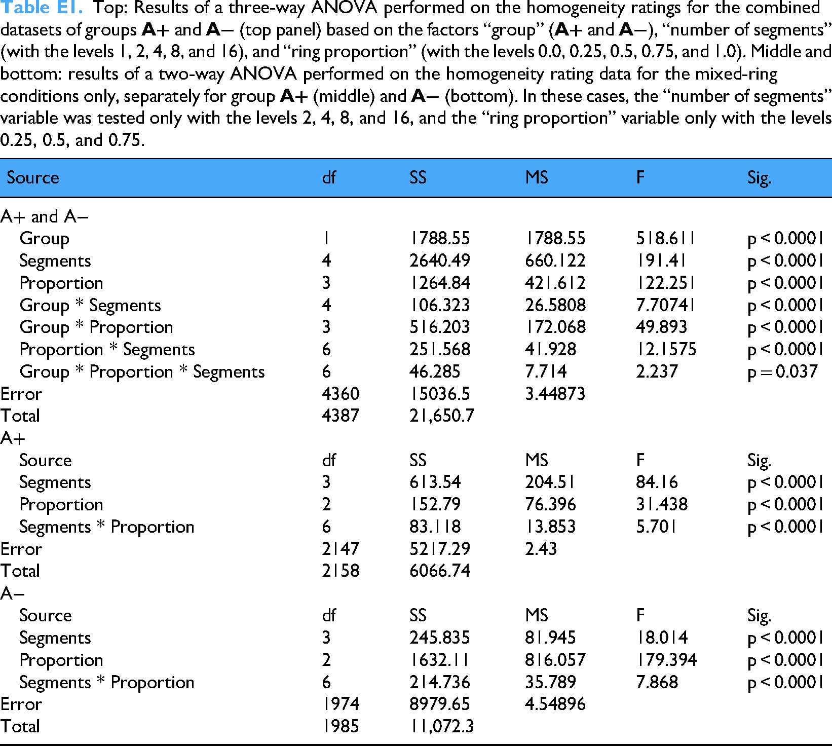
Appendix E. ANOVA Results for the Homogeneity Rating Data
Top: Results of a three-way ANOVA performed on the homogeneity ratings for the combined datasets of groups
| Source | df | SS | MS | F | Sig. |
|---|---|---|---|---|---|
| A+ and A− | |||||
| Group | 1 | 1788.55 | 1788.55 | 518.611 | p < 0.0001 |
| Segments | 4 | 2640.49 | 660.122 | 191.41 | p < 0.0001 |
| Proportion | 3 | 1264.84 | 421.612 | 122.251 | p < 0.0001 |
| Group * Segments | 4 | 106.323 | 26.5808 | 7.70741 | p < 0.0001 |
| Group * Proportion | 3 | 516.203 | 172.068 | 49.893 | p < 0.0001 |
| Proportion * Segments | 6 | 251.568 | 41.928 | 12.1575 | p < 0.0001 |
| Group * Proportion * Segments | 6 | 46.285 | 7.714 | 2.237 | p = 0.037 |
| Error | 4360 | 15036.5 | 3.44873 | ||
| Total | 4387 | 21,650.7 | |||
| A+ | |||||
| Source | df | SS | MS | F | Sig. |
| Segments | 3 | 613.54 | 204.51 | 84.16 | p < 0.0001 |
| Proportion | 2 | 152.79 | 76.396 | 31.438 | p < 0.0001 |
| Segments * Proportion | 6 | 83.118 | 13.853 | 5.701 | p < 0.0001 |
| Error | 2147 | 5217.29 | 2.43 | ||
| Total | 2158 | 6066.74 | |||
| A− | |||||
| Source | df | SS | MS | F | Sig. |
| Segments | 3 | 245.835 | 81.945 | 18.014 | p < 0.0001 |
| Proportion | 2 | 1632.11 | 816.057 | 179.394 | p < 0.0001 |
| Segments * Proportion | 6 | 214.736 | 35.789 | 7.868 | p < 0.0001 |
| Error | 1974 | 8979.65 | 4.54896 | ||
| Total | 1985 | 11,072.3 | |||