Multivariate Logit and Probit models for simultaneous purchases: Presentation,uses,appeal and limitations

Abstract

This article presents Multivariate Logit (MVL) and Probit (MVP) models, which make it possible to analyse simultaneous purchases and relax the restrictive hypothesis that utility maximization leads to a single choice. These models enable a deeper analysis of competitive dynamics in a given category (variety seeking, complementarity, substitutability). The MVL model using a random parameter specification is illustrated in relation to the chocolate category. We underline the advantages and limitations of these models and propose new research avenues.

Keywords

coincidences complementarity cross-effects food products (chocolate)multinomial logit probit multivariate logit probit random parameters simultaneous purchase variety seeking

Introduction

Since the article by Guadagni and Little (1983),¹ the MultiNomial Logit (MNL) model has been a key reference point in modeling (discrete) individual choices within a given product category. It has a great many applications to the field of marketing, particularly in relation to analysis of the impact of marketing action variables on choice (price, promotions, product features, etc.), analysis of market structures, analysis of preferences and conjoint analysis (see for example Aurier, 1993; Desmet, 1993; Erdem, 1996; Fader and Hardie, 1996; Kamakura and Russell, 1994; Krishnamurthi and Raj, 1991). The MNL’s underlying utility model has become the dominant paradigm when it comes to modeling choices (Chandukala et al., 2007).

Yet the MNL model carries significant limitations, mainly because of two highly restrictive hypotheses that it imposes on the choice process. The first, which is the better known of the two and has received more attention in the literature, is the IIA (Independence of Irrelevant Alternatives) hypothesis: given that the probability that an option (product or brand) will be chosen is expressed in terms of the relationship between its utility and the combined utility of the other options belonging to the overall choice set, the MNL model postulates that the relationship between the probabilities of two options i and j ( $\frac{P_{i}}{P_{j}}$ ) is independent of this overall choice set. It depends only on the features of i and j, independently of those of the other available options. As a result, the competitive structure is considered to be perfectly homogenous (equally competitive brands) within the category. This hypothesis is very unrealistic in many situations, which explains why it has been the target of so much criticism. On a market such as chocolate bars, this would suggest that the competition between Lindt and Nestlé is independent of the presence of other brands such as Milka, Crunch or Côte d’Or and their relative products.

Several variants of the MNL model have been developed with a view to relaxing this restrictive hypothesis. The most well-known solutions are the MultiNomial Probit model (MNP; Elrod and Keane, 1995), the hierarchical MNL model (HMNL; McFadden, 1986) and the Nested Logit model (Ben-Akiva and Lerman, 1985). The first of these considers a non-homogenous competitive structure within a given category based on the correlations between the random terms of the products’ utility functions. However, the use of this model suffers from the excessive bulk of its estimation (Greene, 1998). The second is a variant of the MNL model that involves making the overall set of options more homogenous by breaking them down into sub-sets through a hierarchical modeling process divided into several stages. In the case of inter-category choices, for example, this would involve modeling the choice within a particular category from the world of snacks (chocolate, dairy-based deserts, sugary biscuits, etc.), followed by the choice of a brand (lower segment of the hierarchy) based on the choice of one of the categories (e.g. chocolate bars). In the case of intra-category choices, staying with the example of chocolate, it would involve modeling the choice within one of the segments from the category (‘gourmet’, ‘standard’ or ‘cooking’ chocolate, forming the upper segment of the hierarchy) and then conditionally choosing from the various brands that make up the chosen segment (lower segment of the hierarchy). The IIA hypothesis continues to apply to each level of the hierarchy, but it is now more tenable given that the categories have been made more homogenous.

The second limitation has been the subject of much less discussion and was slower to appear in the literature (Simonson, 1990; Harlam and Lodish, 1995; Aurier, 1999; Kim et al., 2002, 2007; Chib et al., 2004; Dubé, 2004; Chandukala et al., 2007). The MNL and MNP models, regardless of which variant is used, use the hypothesis that utility maximisation results in a single choice, or alternatively in the absence of a choice. Behavioural observation has shown that this is not true, particularly in the most common purchasing categories such as food products. A significant proportion of choices are ‘multiple’ in that an individual may choose two, three or more units of choice (products, brands, etc.) from within a given category during a single purchasing session. For example, a consumer may simultaneously choose ‘milk’ chocolate and ‘dark’ chocolate, or ‘cooking’ chocolate and ‘gourmet’ chocolate. One common response to this problem is to deny the multiplicity of choices by arguing that it is the result of several parallel choice processes within various category segments. This has led researchers to study very narrow categories containing a small number of brands (for example ‘gourmet’ chocolate only). Another, equally common response is to eliminate the multiple buyers from the sample on the basis that they are ‘atypical’. Due to the low number of brands and the homogeneity of the competitive structure that emerges from these simplifications, the IIA and single-choice hypotheses are made tenable. Yet such an approach means that some of the competitive dynamic is overlooked: very real albeit non-frontal competition between brands positioned in various segments, the variety-seeking between the products of a single brand’s line that are positioned on different category segments, etc.

The objective of this article is to provide a response to this second limitation. We will present the Multivariate Logit and Probit (MVL and MVP) models for use with multiple choices. We will first look at the structure of MNL and MNP models, before presenting the MVL and MVP models. We will illustrate how they are used in a category of frequently purchased products, i.e. chocolate bars. Finally, we will outline their limitations and future research avenues in this area.

MNL and MNP models

For the last three decades, MNL and MNP models² and their variants have been used to model individual choices. The specificity of a choice is based on its discrete nature (choice or non-choice) in respect of continuous variables such as quantities purchased or market shares. These discrete choices are considered to be a reflection of a non-observable latent variable – probability of choice – which is then modeled.

Model structure

In MNL and MNP models (known as ‘random utility models’ – Greene, 2005), the overall utility U_iht of a unit of choice i (1…I) (product, brand, etc.) for an individual h (1…H) at time t (1…T)³ can be broken down into a deterministic part V_iht (based on the characteristics associated with the unit of choice) and a random part ϵ_iht due to the impact of factors not controlled for in the model:

U_{i h t} = V_{i h t} + ε_{i h t}

(1)

Deterministic utility is expressed as a linear combination of the characteristics of i: the attributes of a product (Fader and Hardie, 1996; Harlam and Lodish, 1995) or brand (Kamakura and Russell, 1994), marketing action variables such as price or advertising (see, for example, Mazumdar and Papatla, 2000; Seetharaman and Chintagunta, 1998), or the individual’s characteristics:

V_{i h t} = α_{i} + β X_{i h t} + γ_{i} Z_{h t}

(2)

Where:

- α_i: constant utility of the choice unit, corresponding to its unique features not taken into account by the model;

- X_iht: vector of the k characteristics of i for h at t (price, presence of promotions, flavour, brand, etc.);

- Z_ht: vector of the j characteristics of h at t (revenue, household size, etc.);

- β and γ_i: vectors of parameters to be estimated.

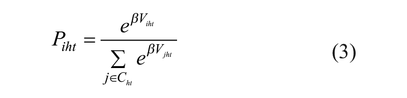
The specification of the law followed by random utility (ϵ_iht in equation (1)) enables the parameters to be estimated: Gumbel’s law⁴ in the case of the MNL model, normal law in the case of MNP. In the former, the probability that unit i will be chosen is expressed as follows (Ben-Akiva and Lerman, 1985):

P_{i h t} = \frac{e^{β V_{i h t}}}{\sum_{j \in C_{h t}} e^{β V_{j h t}}}

(3)

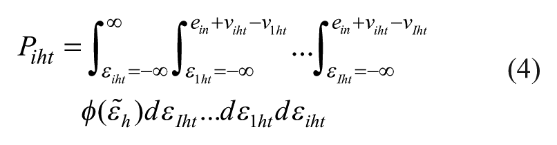
In the latter, it is expressed as follows (Train, 1986):

P_{i h t} = \int_{ε_{i h t} = - \infty}^{\infty} \int_{ε_{1 h t} = - \infty}^{e_{i n} + v_{i h t} - v_{1 h t}} \dots \int_{ε_{I h t} = - \infty}^{e_{i n} + v_{i h t} - v_{I h t}} Φ ({\tilde{ε}}_{h}) d ε_{I h t} \dots d ε_{1 h t} d ε_{i h t}

(4)

Where:

- ${\tilde{ε}}_{h}$ : vector of the random components of the utility function, ${\tilde{ε}}_{h} = [\begin{matrix} ε_{1 h t}, & \dots, & ε_{I h t} \end{matrix}]$ , distributed according to a multivariate normal law with mean 0, variance-covariance matrix Σ and size I × I, $Σ = [\begin{matrix} σ_{11} & \dots & ρ_{I 1} \\ \dots & \dots & \dots \\ ρ_{1 I} & \dots & σ_{I I} \end{matrix}] .$ .

Two significant differences should be noted here. First, in the MNL model (3), random variables ϵ_iht are considered to be independent ( $cov [ε_{i}, ε_{j}] = 0$ ), while they can be correlated ( $cov [ε_{i}, ε_{j}] = ρ_{i j}$ ) in the MNP model (4). It is for this reason that the MNL model is based on the IIA hypothesis:

\frac{P_{i h t}}{P_{j h t}} = \frac{\exp (β V_{i h t}) / \sum_{k} \exp (β V_{k h t})}{\exp (β V_{j h t}) / \sum_{k} \exp (β V_{k h t})} = \frac{\exp (β V_{i h t})}{\exp (β V_{j h t})}

(5)

This means that the ratio between two choice units is affected only by their characteristics, regardless of those of the other available choice units and the size of the overall choice set. Second, using Gumbel’s distribution, the MNL model can be directly expressed and calculated, whereas the MNP model gives estimates based on numeric calculations (McFadden, 1986). These two differences are not insignificant where the size of the overall choice set increases. In practice, beyond four or five units of choice, researchers tend to use the MNL model, despite improvements in the calculation capabilities of computers.

Limitation of MNL and MNP models

In these models, individuals make just one choice each time, that which maximizes utility. These so-called ‘pick one’ models are therefore based on the hypothesis that the consumer makes a single choice from an overall choice set (Dubé, 2004; Walsh, 1995). This constitutes a limitation both in theoretical and practical terms, as reality tells us that this hypothesis is often unrealistic and serves only to artificially restrict the overall choice set facing the consumer.

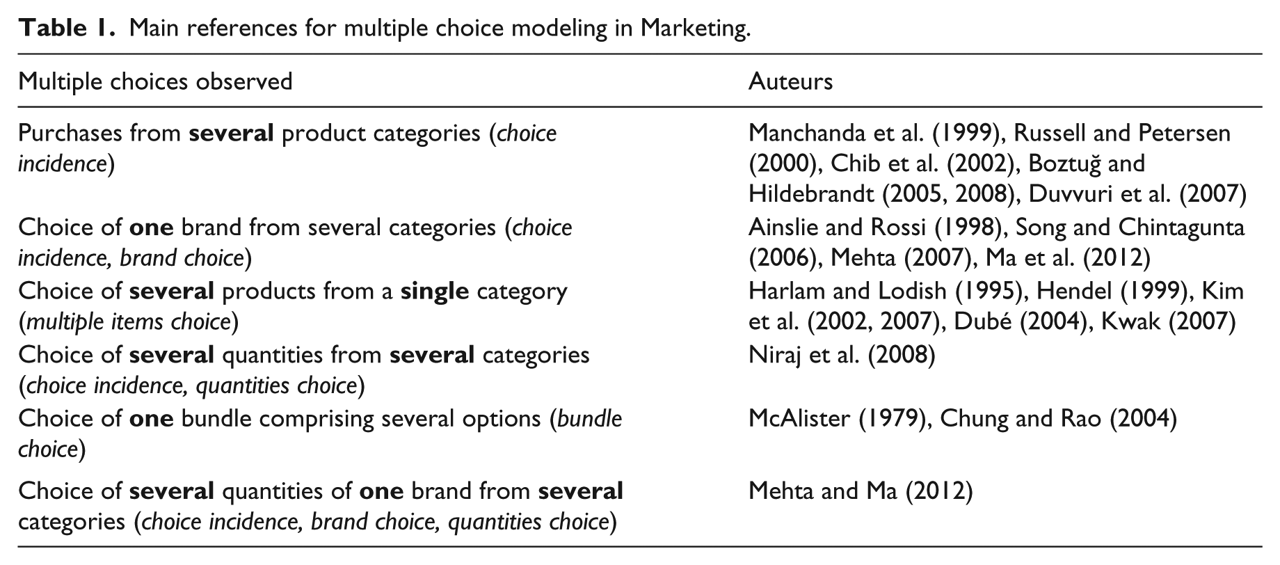
During a single shopping trip, an individual may purchase several products from several different product categories (multi-category choices), and these purchases cannot be considered to be independent of one another (Manchanda et al., 1999; Mehta, 2007; Mehta and Ma, 2012). An individual may also purchase several products from within a single category (intra-category choices; see Chandukala et al., 2007; and Kim et al., 2002, 2007), especially where this category carries a sufficiently broad definition (e.g. chocolate bars). It is therefore no longer possible to postulate that utility maximization results in single and independent choices. In fact, there may be structural links between the different chosen units (McAlister, 1979). For example, when making a multi-category choice, the purchase of a cake mix may be linked to the purchase of frosting (Ma et al., 2012), the purchase of eggs may be linked to the purchase of bacon (Niraj et al., 2008), or the purchase of pasta may be linked to the chosen sauce (Mehta and Ma, 2012). When making an intra-category choice, an individual may purchase both white and red wine, both traditional and diet soda and various flavored crisps in anticipation of different consumption contexts or the need for variety or because the household concerned includes several people with different preferences (Laurent, 1978; Aurier, 1991, 1999; Dubé, 2004; Mejía, 2012). Table 1 outlines the main types of models for multiple choices currently available in the marketing literature.

Table 1.

Main references for multiple choice modeling in Marketing.

Multiple choices observed	Auteurs
Purchases from several product categories (choice incidence)	Manchanda et al. (1999), Russell and Petersen (2000), Chib et al. (2002), Boztuğ and Hildebrandt (2005, 2008), Duvvuri et al. (2007)
Choice of one brand from several categories (choice incidence, brand choice)	Ainslie and Rossi (1998), Song and Chintagunta (2006), Mehta (2007), Ma et al. (2012)
Choice of several products from a single category (multiple items choice)	Harlam and Lodish (1995), Hendel (1999), Kim et al. (2002, 2007), Dubé (2004), Kwak (2007)
Choice of several quantities from several categories (choice incidence, quantities choice)	Niraj et al. (2008)
Choice of one bundle comprising several options (bundle choice)	McAlister (1979), Chung and Rao (2004)
Choice of several quantities of one brand from several categories (choice incidence, brand choice, quantities choice)	Mehta and Ma (2012)

Multivariate Logit and Probit models

MVL and MVP, or so-called ‘pick any’ models were developed in the 2000s with a view to analyzing multiple choices. However, the theoretical postulates on which they are based have been around for much longer (see Besag, 1974 or Cox, 1972 in the case of the MVL). According to the binary Logit or Probit model, consumers face a single option that they can either choose or reject. By generalizing this principle to several simultaneous choices, the observed variable becomes a ‘basket’ made up of binary choices (yes/no; yes/no, and so on). Multivariate models are therefore extensions of the binary Logit and Probit models.

The ‘basket’ concept

Besag’s theorem (1974)⁵ laid the foundations for multivariate models: if the probability that each element in a set exists is greater than zero (condition of positivity) and if each element is dependent on the other elements that belong to that set (condition of dependence), it is possible to calculate the joint probability of the different elements. In the case of multiple choices between different products, this means that if each product can be chosen individually (for example because it is available on the shelves) and if each product can be considered dependent on the others then there is also a joint probability that I products will be chosen.

Let us consider the example of basket b (1…B) containing up to I choice units i (1…I). Purchaser h (1…H) at t (1…T) may include 0, 1, 2 …. I choice units. Each element in basket b is represented by a binary variable $y_{i h t}^{b}$ , which is coded as 1 if i is present (regardless of quantity). This gives us a vector with I components, $y_{h t}^{b} = {y_{1 h t}^{b}, y_{2 h t}^{b}, \dots, y_{I h t}^{b}}$ , representing the I binary choices/non-choices that make up h’s basket b at t. With I choice units, there are two to the power of I (2^I) distinct baskets. For example, where there are three products (A, B and C), there are 2³ = 8 distinct baskets, including a null basket in which there is no choice:

[A, 0, 0], [0, B, 0], [0, 0, C], [A, B, 0], [A, 0, C], [0, B, C], [A, B, C], [0, 0, 0]

(6)

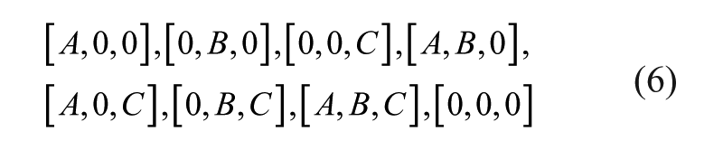
The null basket is not problematic in theoretical terms, but it is usually excluded from the model in practice as there must have been a purchase in the category (Russell and Petersen, 2000; Boztuğ and Hildebrandt, 2005, 2008).

Specification of the utility function

The utility function of a choice unit within a basket is identical to that which was expressed in (1) in the case of MNL and MNP models. As a result, the specificities that resulted from choosing Gumbel’s law or the normal law (equations (3) and (4)) apply to the MVL and MVP models, which are extensions of the binary Logit and Probit models.

In the simplest (and most reductive) version, the deterministic utility (V_iht) of i is expressed as a linear combination of its characteristics (independently of those of the other choice units in the category) and those of the individual:

V_{i h t} = β_{i} X_{i h t}

(7)

Where:

- X_iht: vector of the characteristics of i, for h at t, and the characteristics of h;

- β_i: vector of the associated coefficients to be estimated.

In this case, the resolution of the multivariate model is equivalent to that of I independent binary models expressing the purchase/non-purchase of each of the elements in the basket.

However, the presence of simultaneous purchases in a category is usually the expression of interactions between the different choice units (Ma et al., 2012): cross-effects and coincidences that it is therefore useful to integrate into the model.

Cross-effects (or ‘complementarities’): these correspond to the competitive interactions that are due to the use of marketing levers, in particular pricing and promotions (Manchanda et al., 1999). For example, due to a promotion on ‘cooking’ chocolate, the consumer may decide to make an additional purchase of ‘gourmet’ chocolate. The impact of the characteristics of the other choice units (j) is therefore integrated into the utility function of i:

V_{i h t} = β_{i} X_{i h t} + \sum_{j \neq i} ψ_{j} X_{j h t}

(8)

Where:

- X_jht: vector of the characteristics of j and h;

- ψ_j: vector of the associated coefficients, measuring the impact of each characteristic of j on the deterministic utility of i.

Taking these complementarities into account adds k * I * (I – 1) parameters to the utility function.

Purchasing coincidences: these correspond to a form of complementarity that is not directly brought about by marketing actions. For example, if a consumer purchases ‘milk’ chocolate for their children and ‘dark’ chocolate for themselves, the combined purchase is a result of the composition of the household. This means that purchasing coincidences can be an expression of a purchasing style (an individual who systematically chooses several products), the heterogeneity of preferences within the household, etc., resulting in the simultaneous purchase of several different products. The way in which these coincidences are taken into account differs between the MVL and MVP models. They are naturally integrated in the case of the MVP model into the covariance matrix between the random utilities ϵ_iht (equation (4)). In the MVL model, due to the hypothesis about the independence of random utilities, coincidences must be added to the deterministic utility function (Russell and Petersen, 2000):

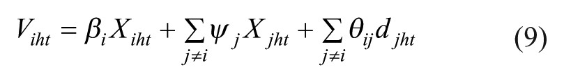
V_{i h t} = β_{i} X_{i h t} + \sum_{j \neq i} ψ_{j} X_{j h t} + \sum_{j \neq i} θ_{i j} d_{j h t}

(9)

Where:

- d_jht: binary variable coded as 1 if j is included in h’s basket at t, and 0 otherwise;

- θ_ij: associated coefficient, measuring the impact of the coincidence on the probability that i will be chosen.

Two restrictions are imposed on θ_ij: θ_ii = 0 for the identification of the model and θ_ij = θ_ji as co-presence is a symmetrical indicator. With I choice units, there are I * (I – 1) / 2 indicators of co-presence.

The significance of coincidences differs in the MVP and MVL models (Niraj et al., 2008). In the former, because it is based on the correlations between random utilities, it is integrated into all of the non-observed elements that resulted in the simultaneous purchase of two units. In the latter, because the coincidence is integrated with the indicator of co-presence, it is only included in the case of a joint purchase of two products. This difference may modify both the importance and significance of coincidences (Seetharaman et al., 2005).

Taking account of the heterogeneity of preferences

Taking heterogeneity (of individuals, retail outlets, etc.) into account involves relaxing the hypothesis of a single value (homogeneity) of a coefficient within the population. Several solutions have been put forward in the case of MNL and MNP models, chief among them being latent class models and random parameter models: see Ma et al. (2012) for an example of a latent class MVP model, and Duvvuri et al. (2007) for an example of a random parameter MVP model.

Latent class models deal with heterogeneity by considering the population to be divided up into Q classes of individuals. They estimate Q coefficients for each parameter (1 per class) and retain the hypothesis of homogeneity in each class (Kamakura and Russell, 1989, 1994; Fader and Hardie, 1996). Random parameter models consider heterogeneity to be ‘continuous’: the inter-individual variations of a given parameter are distributed using a statistical law that is specified beforehand, often the normal law (Chintagunta et al., 1991; Dubé et al., 2010). Inter-individual variations may come from two sources (Revelt and Train, 1997; Bonnet, 2004; Horsky et al., 2004): the first is unknown and therefore not observed by the researcher (specific tastes, preference for a particular brand, etc.), while the second is related to specific characteristics observed by the researcher (household size, revenue, etc.).

In our empirical application, we used a random parameter model. By relaxing the homogeneity hypothesis, each individual has a specific value β_h which deviates from the mean coefficient β according to the normal law. β_h is then expressed as a function of individual observed characteristics z_h, which then explain part of the deviation from β (Greene, 2005):

β_{h} = β + δ z_{h} + σ v_{h}

(10)

Where:

- β_h: coefficient associated with h, such that $β_{h} \sim N [β + δ z_{h}, σ ²]$ ;

- σ: standard deviation of β_h from β;

- β: mean coefficient in the sample;

- z_h: characteristic of h;

- δ: coefficient measuring the impact of z_h on β_h,;

- ν_h: individual heterogeneity, non-observed, standardized.

It should be noted that this heterogeneity can be applied to the utility of each product (coefficients β_i), to complementarities (coefficients ψ_j; see for example Manchanda et al., 1999) and coincidences (coefficients θ_ij).

Model estimation

For basket b as a whole, the overall utility function μ_bht is expressed as the sum of the individual utilities of the i choice units.

In the case of the multivariate Logit model, the utility of basket b is expressed as follows:

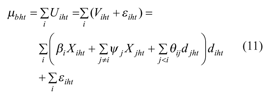
μ_{b h t} = \sum_{i} U_{i h t} = \sum_{i} (V_{i h t} + ε_{i h t}) = \sum_{i} (β_{i} X_{i h t} + \sum_{j \neq i} ψ_{j} X_{j h t} + \sum_{j < i} θ_{i j} d_{j h t}) d_{i h t} + \sum_{i} ε_{i h t}

(11)

Where:

- X_iht (X_jht): vectors of the characteristics of option i (j);

- β_i and ψ_j: vectors of the associated coefficients;

- d_iht (d_jht): binary variable coded as 1 if i (j) is included in the basket, 0 otherwise;

- $θ_{i j}$ : coefficient for the co-presence of i and j.

In the case of the multivariate Probit model, the basket’s utility is expressed as follows:

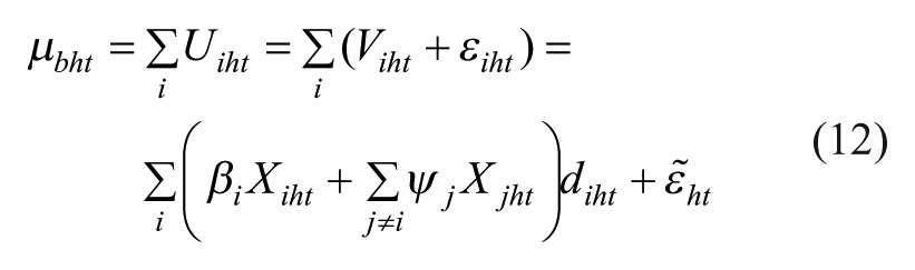
μ_{b h t} = \sum_{i} U_{i h t} = \sum_{i} (V_{i h t} + ε_{i h t}) = \sum_{i} (β_{i} X_{i h t} + \sum_{j \neq i} ψ_{j} X_{j h t}) d_{i h t} + {\tilde{ε}}_{h t}

(12)

Where:

- X_iht (X_jht): vectors of the characteristics of i (j);

- d_iht (d_jht): variable coded as 1 if i (j) is included in the basket;

- β_i et ψ_j: associated coefficients;

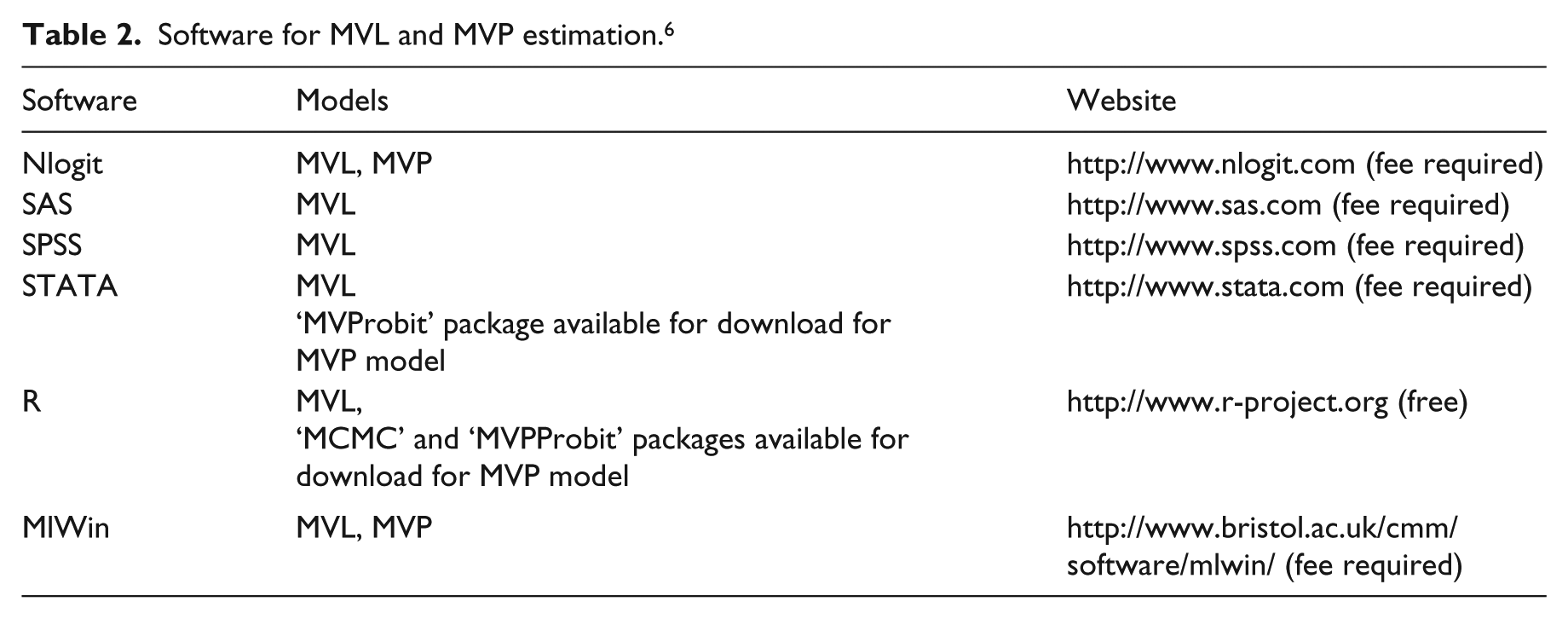
- ${\tilde{ε}}_{h t}$ : vector of the random components distributed according to a multivariate normal law, ${\tilde{ε}}_{h t} \sim M V N (0, Σ)$ where Σ is the matrix for variances-covariances between the basket’s I random utilities.

The estimation is reached using the maximum log-likelihood method (LL). As in the case of the MNL model, the likelihood function in the MVL model may be expressed analytically and calculated (closed version of Gumbel’s law of distribution). With both the MVP and MNP models, it is necessary to use the simulated maximum likelihood (SML) method because the normal law is being used (Niraj et al., 2008). The appeal of the MVL model, therefore, is that it can be estimated using any software that enables MNL model estimation. In contrast, the MVP model requires the use of more sophisticated techniques such as the Monte Carlo Markov Chain (MCMC), which enables the approximation of multivariate normal I distributions (see Chib et al., 1998 for the use of MCMC with MNP, and Chib and Greenberg, 1998 in the case of MVP). Table 2 presents the different software programs that can be used for the resolution of MVL and MVP models.

Table 2.

Software for MVL and MVP estimation.⁶

Software	Models	Website
Nlogit	MVL, MVP	http://www.nlogit.com (fee required)
SAS	MVL	http://www.sas.com (fee required)
SPSS	MVL	http://www.spss.com (fee required)
STATA	MVL ‘MVProbit’ package available for download for MVP model	http://www.stata.com (fee required)
R	MVL, ‘MCMC’ and ‘MVPProbit’ packages available for download for MVP model	http://www.r-project.org (free)
MlWin	MVL, MVP	http://www.bristol.ac.uk/cmm/software/mlwin/ (fee required)

The use of multivariate choice models in the literature

The multivariate models presented above represent the simplest forms. Current developments distinguish between several different levels of choice. In the case of inter-category choices, this means choosing or rejecting a particular category and then choosing or rejecting a given product within the chosen category, whereby at each level a multinomial (1 from a set) or multivariate (1 or more from the set) approach is applied (Seetharaman et al., 2005). In the case of intra-category choices, one analyses the choice of one or several brands and, for each chosen brand, the choice of one or several products. This represents a very realistic extension of models for individual choices.

Table 3 presents the multivariate models identified in the marketing literature. These models are attractive from a theoretical viewpoint as they can easily integrate several interactions between choice units at different levels. Their limitations should nonetheless be pointed out from a practical perspective. An increase in the number of choice units rapidly increases the complexity of the required calculations: for I units described according to k characteristics, there are 2^I different possible baskets to be modeled, I * (I − 1) / 2 coincidences and I * (I − 1) * k cross-effects to be integrated. Where k = 2 (pricing and promotions) and I = 4, this gives 16 baskets, 6 coincidences and 24 cross-effects. Where I = 5, the number of baskets increases to 32, with 10 coincidences and 40 cross-effects. Where I = 6, the model includes 64 baskets, 15 coincidences and 60 cross-effects, and so on. Applications are therefore limited to four to six units of choice and/or include restrictions that limit the number of parameters and/or combinations (Kwak, 2007; Ma et al., 2012; Mehta, 2007). For example, Kwak (2007) produces a multivariate model of the choice between six flavours and two brands, which represents 2¹² theoretical combinations. Given that consumers may choose one or more flavours within a single brand, the number of combinations is reduced to 2 * 2⁶.

Table 3.

The different multivariate models identified in the marketing literature.

Authors	Structure	Dependent variable	Interactions
Manchanda et al. (1999)	Multivariate probit	4 product categories	Cross-effects and coincidences
Russell and Petersen (2000)	Multivariate logit	4 product categories	Coincidences
Erdem and Sun (2002)	Bivariate multinomial probit	2 categories with 1 product in each category	Cross-effects between categories and within a category, coincidences between categories
Song and Chintagunta (2006)	Multivariate logit – multinomial	4 categories with 1 brand per category	Coincidences and cross-effects between categories
Duvvuri et al. (2007)	Multivariate probit	6 categories	Coincidences and cross-effects
Kwak (2007)	Multinomial logit – multivariate	1 brand and 1 or more products of the brand	Coincidences between products
Iyer and Seetharaman (2008)	Trivariate logit	‘Pricing’ strategies, ‘objective’ and ‘subjective’ quality (low vs. high)	Correlations (coincidences) between the three strategies
Niraj et al. (2008)	Bivariate logit – binomial	2 categories and one quantity (1 or 2)	Cross-effects between categories and conjoint utility of multiple basket (2 quantities in 2 categories)
Ma et al. (2012)	Bivariate logit – multinomial	2 categories and 1 brand in each category	Cross-effects and coincidences between brands and between categories, coincidences between brands within a single category

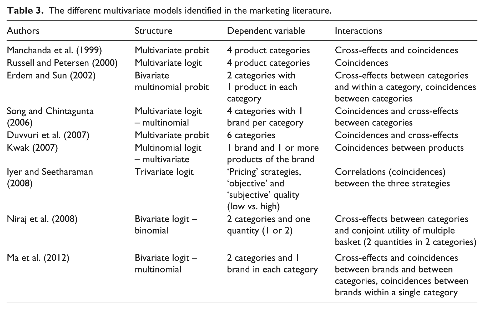
The possibilities for multivariate models are very wide in scope and depend on the researcher’s chosen objective: intra- or inter-category choices, controlling for the impact of cross-effects and coincidences. The available data has an influence on the possible analyses. The development of multivariate ‘cross-category’ models is therefore linked to the simultaneous collection of data in several different categories (Chib et al., 2002). Finally, the desired level of complexity will determine which model should be used (simple or multilevel multivariate model). It should be noted that Table 3 is not intended as a guide, but rather a (non-exhaustive) reflection of the way in which multivariate models are used. The application of these models is not limited to panel data alone: the data contained in the customer files of companies and of course the data compiled from choices made online (retailing websites) are just as (if not more) suitable as they provide information about historic multiple choices at both intra- and inter-category levels. We would welcome the development of applications using such data.

Illustration: Modeling simultaneous purchases in the category of chocolate bars

We present a random parameter intra-category MVL model. In contrast to the vast majority of applications, which are inter-category (where multiple choices made from several different categories are modeled), we have adopted an intra-category approach. It is common for consumers to make simultaneous purchases from within a single category during a single purchasing session (see for example Walsh, 1995; Kim et al., 2002; Dubé, 2004).

Analyzed data

The data used comes from a panel generated by MarketingScan in the category of chocolate bars, relating to a period from 31 December 2007 to 25 September 2010 (143 weeks) in 21 retail outlets located in two closed zones in France. From a total of 64,699 purchases (representing 55,600 purchasing sessions) and after the elimination of mono-purchasers who never buy more than one product during a single session (4132 purchasers and 18,987 purchases), the total sample is made up of ‘multiple’ purchasers who on at least one occasion made multiple purchases during the period observed, i.e. 2327 panellists (36%), representing 36,613 purchasing sessions and 45,712 purchases (66% and 71% of sessions and purchases respectively). It is worth noting that although they are fewer in number (one third of consumers), the multiple purchasers made more than two-thirds of all purchases, all the more reason to include them in the model. From this overall set, we observed 7572 multiple-purchase sessions (21% of all sessions), covering 16,671 multiple choices (36% of purchases), an average of 2.2 multiple purchases per session. These figures are lower than those reported in other research studies. Harlam and Lodish (1995), for example, observed 69% of multiple-purchase sessions, and Dubé (2004), 30%.

In the interest of clear pedagogy, so as to simplify the interpretation of the findings, we considered the choice unit to be the brand. This reduces the overall set of choices but also the number of simultaneous purchases observed, given that many simultaneous purchases are made up of products from a single brand (Mejía, 2012). Three brands were selected – Lindt, Nestlé and Milka – representing more than 90% of purchases, with the other brands placed in the ‘Other’ category.⁷ This gave us 15 valid baskets. In order to reduce the calculation time (this application was primarily intended as an illustration), we decreased the size of the sample, retaining only those panelists involved in at least six multiple-purchase sessions, giving us a final sample of 136 panelists representing 6521 purchasing sessions (26% of which were multiple-purchase sessions) and 8340 purchases (42% of which were multiple purchases). The poor representativity of this sample is compensated for by a higher rate of multiple purchases, making our estimates more robust. Figure 1 presents the composition and frequency of purchase of each basket as a proportion of the overall set of purchasing sessions. The numbers 1, 2, 3 and 4 correspond respectively to the Nestlé, Lindt, Milka and ‘Other’ brands: number 12 indicates the basket simultaneously containing the Nestlé and Lindt brands; this represents 7.5% of purchasing sessions (490) and 11.75% of purchases (980).

Figure 1.

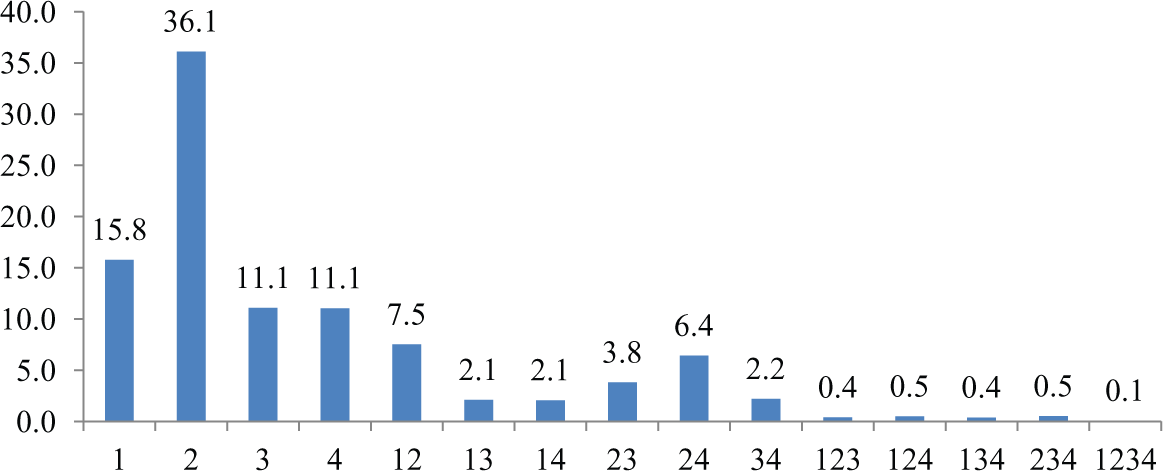
Content and frequency of baskets (total: 6521).

We observed a high proportion of single-brand baskets (baskets 1, 2, 3 and 4, representing 74% of all baskets), with around 25% containing more than one brand (mostly no more than two).⁸

Model estimation

The deterministic utility function of brand i (1…I) for household h (1…H) at t (1…T) is expressed as follows (we have removed h and t for improved readability):

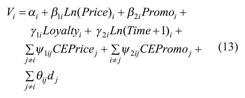
\begin{array}{l} V_{i} = α_{i} + β_{1 i} L n {(P r i c e)}_{i} + β_{2 i} P r o m o_{i} + γ_{1 i} L o y a l t y_{i} + γ_{2 i} L n {(T i m e + 1)}_{i} \\ + \sum_{j \neq i} ψ_{1 i j} C E P r i c e_{j} + \sum_{i \neq j} ψ_{2 i j} C E P r o m o_{j} + \sum_{j \neq i} θ_{i j} d_{j} \end{array}

(13)

Where:

- α_i: constant measuring the intrinsic utility of brand i;

- Ln(Price)_i: logarithm of the price of i at t;

- Promo_i: binary variable coded as 1 where promotional activities are present (product facing and/or in-store entertainment and/or price reductions) for i at t;⁹

- β_1i and β_2i: coefficients to be estimated, measuring the impact of price and promotions on the utility of i;

- Loyalty_i: behavioural loyalty to brand i for purchaser h representing past choices of i (Dubé et al., 2010). Loyalty is an important variable in discrete choice models as it has a high explicative value and enables the researcher to pick up on some inter-individual variations (Guadagni and Little, 1983, Kamakura and Russell, 1994, Erdem, 1996). Here it is measured as a logarithm of the number of purchasing sessions (excluding the current session) in which brand i was purchased (Fader, 1993). This function is set to 0 for each individual;

- γ_1i: coefficient measuring the impact of loyalty on the utility of i;

- Ln(Time + 1)_i: logarithm of the time elapsed since the last purchase of i, expressed in weeks, comparable to the notion of ‘recency’;

- γ_2i: coefficient measuring the impact of the time elapsed on the utility of i;

- CEPrice_j and CEPromo_j: cross-effects (equation (8)) measuring the impact of the characteristics of the other brands (j) on the utility of i;

- ψ_1ij and ψ_2ij: coefficients measuring the impact of these characteristics on the utility of i;

- θ_ij: coefficient measuring the impact of purchase coincidences involving i and j (equation (9));

- d_j: binary variable coded as 1 when j is included in h’s basket at t.

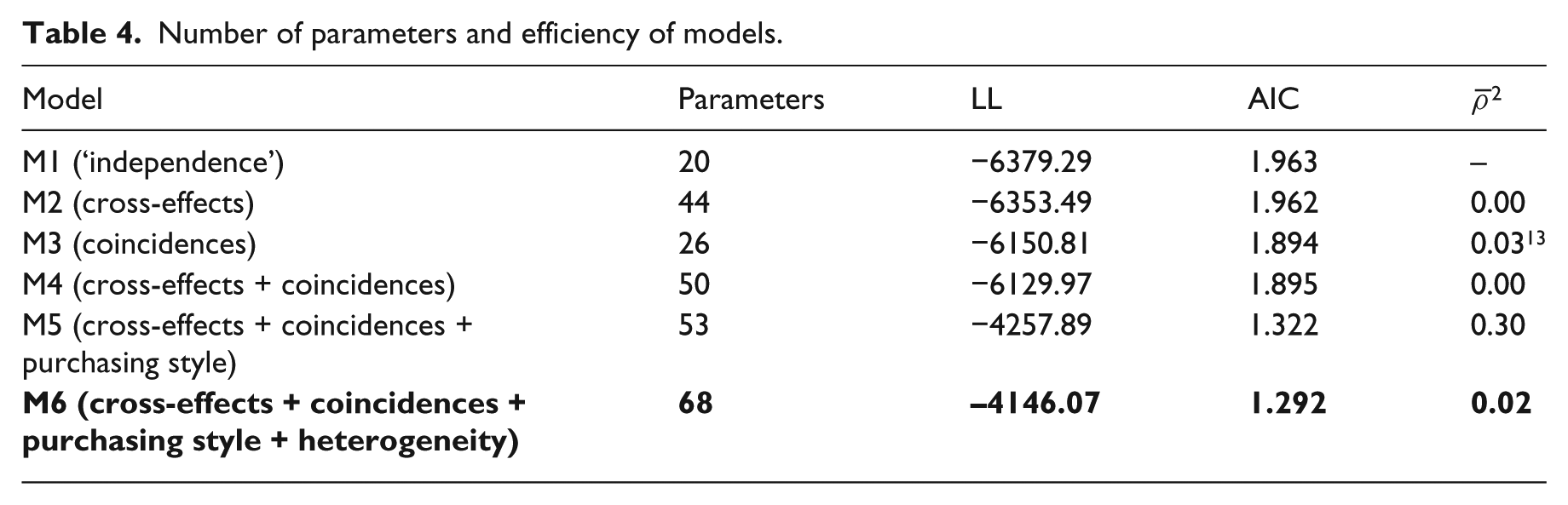
We successively estimated six models (M1 to M6). M4 is the complete model defined in equation (13), the formulation of which is provided in equation (11). Other simpler models are used by way of comparison: M1 represents the ‘independent’ model expressed in equation (7). It corresponds to the estimation of four simultaneous binary Logit models (one for each brand), thereby allowing us to test the benchmark MNL model so it can be compared to the MVL models (M2 to M6). M2 integrates the cross-effects (equation (8)), while M3 integrates the coincidences (equation (9)) by reducing the cross-effects to 0. M4 simultaneously integrates the cross-effects and coincidences. M5 builds on M4 by integrating the impact of three individual characteristics (frequency of purchase, time elapsed since last session and size of basket) into the coincidences equation, as in Russell and Petersen (2000):

θ_{i j} = δ_{i j} + υ F r e q_{h} + τ Q u a n_{h} + η \ln (L a g_{h})

(14)

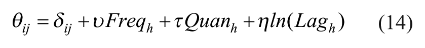
Where:

- δ_ij: coefficient of coincidence between i and j to be estimated, net of the effects of individual characteristics;

- Freq_h: average frequency of purchase of household h (average number of purchasing sessions per week) over the study period;

- Quan_h: average quantities purchased by h over the study period (number of products / number of purchasing sessions);

- ln(Lag_ht): logarithm of the time elapsed since the last purchasing session;

- υ, τ and η: coefficients to be estimated, representing the impact of these individual variables on coincidences.

This equation takes into account the purchasing style of consumers, which may explain the combined purchase of several products. The coefficients υ, τ and η are identical regardless of coincidences; this means they measure the utility of making multiple purchases compared to a single choice.¹⁰

Finally, M6 is a random parameter model that builds on M5 by controlling for inter-individual heterogeneity: the coefficients δ_ij, ν, τ and η vary according to the size of the household (equation 10). We believe that household size has an impact on coincidences (for example, the purchase of ‘adult’ and ‘children’s’ brands simultaneously) and purchasing style.

The software application used is Nlogit 4 (Greene, 2008), and the procedure is presented in Appendix 1. The advantage of this application is its considerable flexibility: e.g. different forms of heterogeneity can be taken into account, and MVP models can be directly estimated. In our experience, its main weakness is that the time required for calculations can be extremely long: several days for a random parameter MNL model estimated using a standard laptop!

Table 4 displays the goodness of fit for each model: number of parameters, maximum log likelihood (LL), AIC¹¹ and $\bar{ρ} ²$ ¹² efficiency criteria (Ben-Akiva and Lerman, 1985). The most efficient model minimizes the AIC. $\bar{ρ} ²$ is an indicator of the ‘incremental’ performance of a model containing more parameters than more parsimonious models.

Table 4.

Number of parameters and efficiency of models.

Model	Parameters	LL	AIC	$\bar{ρ} ²$
M1 (‘independence’)	20	−6379.29	1.963	–
M2 (cross-effects)	44	−6353.49	1.962	0.00
M3 (coincidences)	26	−6150.81	1.894	0.03¹³
M4 (cross-effects + coincidences)	50	−6129.97	1.895	0.00
M5 (cross-effects + coincidences + purchasing style)	53	−4257.89	1.322	0.30
M6 (cross-effects + coincidences + purchasing style + heterogeneity)	68	–4146.07	1.292	0.02

Analysis of findings

Table 4 makes it clear that the integration of cross-effects in M2 does not improve M1 ( $\bar{ρ} ²$ = 0.00), perhaps because of the high number of parameters it generates (24) and because of the aggregation of choice units. However, the integration of coincidences (M3 compared to M1) significantly improves the model ( $\bar{ρ} ²$ = 0.03). This finding shows that the MVL model surpasses the MNL model. M5, which controls for the effect of purchasing ‘style’ (frequency, quantities and time elapsed) on coincidences, constitutes the greatest improvement of the model ( $\bar{ρ} ²$ = 0.30). Finally, the inter-individual heterogeneity integrated into M6 further improves the model’s goodness of fit ( $\bar{ρ} ²$ = 0.02).

Estimated coefficients in M6

Tables 5 to 8 display all of the model’s coefficients.

Table 5.

Utility function. Estimated coefficients (standard deviations).

	Nestlé	Lindt	Milka	‘Other’
Constant	–2.83 (0.75) **	–2.81 (0.75) **	–3.08 (0.76) **	–2.93 (0.76) **
Loyalty	0.59 (0.06) **	0.58 (0.06) **	0.66 (0.07) **	0.59 (0.07) **
Time	–8.67 (0.40) **	–8.69 (0.40) **	–8.54 (0.40) **	–8.61 (0.40) **

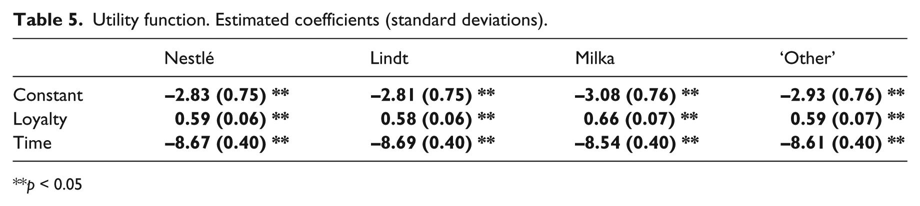
p < 0.05

Table 6.

‘Pricing’ cross-effects. Estimated coefficients (standard deviations).

		Impact of pricing of
		Nestlé	Lindt	Milka	‘Other’
On the utility of	Nestlé	−0.54 (0.36)	0.62 (0.44)	−0.56 (0.40)	−0.56 (0.38)
	Lindt	0.37 (0.33)	0.21 (0.41)	–1.04 (0.37) **	–1.06 (0.36) **
	Milka	−0.23 (0.39)	0.16 (0.49)	–0.90 (0.04) **	–0.81 (0.43) *
	‘Other’	0.16 (0.38)	0.88 (0.47) *	–1.01 (0.42) **	–1.45 (0.41) **

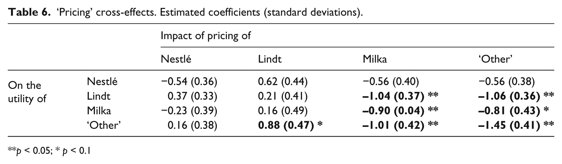
p < 0.05; * p < 0.1

Table 7.

‘Promotions’ cross-effects. Estimated coefficients (standard deviations).

		Impact of promotions by
		Nestlé	Lindt	Milka	‘Other’
On the utility of	Nestlé	−0.01 (0.29)	0.09 (0.19)	0.46 (0.34)	–0.74 (0.24) **
	Lindt	0.01 (0.27)	0.45 (0.18) **	0.17 (0.32)	–0.83 (0.22) **
	Milka	0.21 (0.31)	0.22 (0.21)	0.18 (0.37)	–0.98 (0.26) **
	‘Other’	0.21 (0.30)	−0.23 (0.20)	0.38 (0.36)	–0.65 (0.25) **

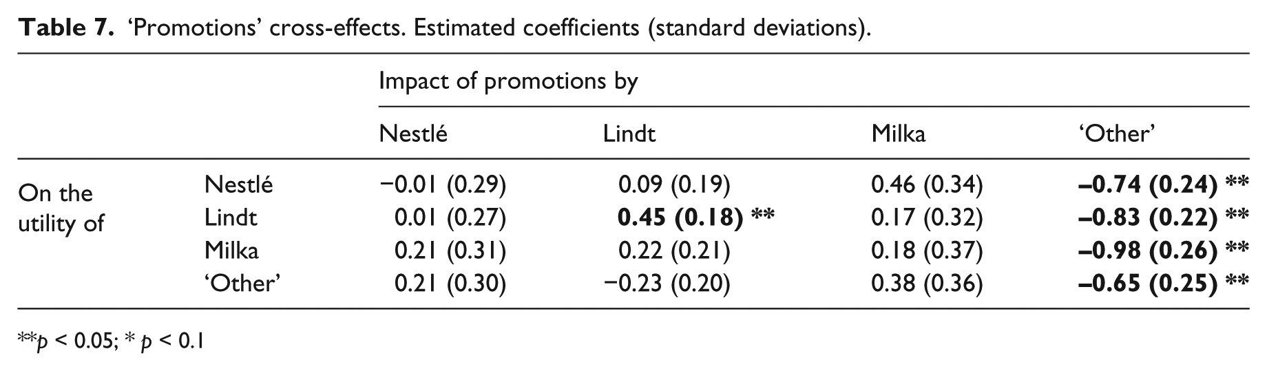
p < 0.05; * p < 0.1

Table 8.

Coincidences between brands, purchasing style and inter-individual heterogeneity. Estimated coefficients (standard deviations).

	Nestlé	Lindt	Milka	‘Other’
Frequency of purchase	–5.05 (1.06) **
δ_{household size}	0.13 (0.27)
σ_population	4.75 (0.44) **
Quantity purchased	0.61 (0.22) **
δ_{household size}	–0.05 (0.06)
σ_population	0.19 (0.17)
Time since last purchase	8.19 (0.14) **
δ_{household size}	0.03 (0.06)
σ_population	0.13 (0.13)
Nestlé		2.94 (0.62) **	2.09 (0.95) **	2.35 (0.63) **
δ_{household size}		0.02 (0.10)	0.07 (0.20) **	−0.20 (0.14)
σ_population		1.25 (0.29) **	4.03 (0.64) **	2.45 (0.29) **
Lindt	2.94 (0.62) **		2.33 (0.65) **	1.76 (0.58) **
δ_{household size}	0.02 (0.10)		0.04 (0.11)	0.17 (0.11)

σ_population	1.25 (0.29) **		1.25 (0.29) **	2.45 (0.29) **
Milka	–2.09 (0.95) **	2.33 (0.65) **		1.74 (0.67) **
δ_{household size}	0.07 (0.20) **	0.04 (0.11)		0.15 (0.14)
σ_population	4.03 (0.64) **	1.25 (0.29) **		2.45 (0.29) **
‘Other’	2.35 (0.63) **	1.76 (0.58) **	1.74 (0.67) **
δ_{household size}	−0.20 (0.14)	0.17 (0.11)	0.15 (0.14)
σ_population	2.45 (0.29) **	2.45 (0.29) **	2.45 (0.29) **

p < 0.05; * p < 0.1

All of the coefficients associated with loyalty are positive and significant, underscoring the impact of loyalty on the probability that a given brand will be purchased. Conversely, all of the coefficients associated with the time elapsed since the last purchase are negative: the greater the duration, the lower the likelihood of a purchase, as the brand is progressively removed from the consumer’s consideration and overall choice set.

Tables 6 to 7 display the effects (simple and cross) of pricing and promotions on the probability that a brand will be chosen (the diagonal shows simple effects). Five coefficients of the cross-effects of pricing are significant: Milka → Lindt (-1.04), ‘Other’ → Lindt (-1.06), ‘Other’ → Milka (-0.81), Lindt → ‘Other’ (0.88) and Milka → ‘Other’ (-1.01). In a reversal of the other cross-effects, in relation to ‘pricing’ complementarities, a positive coefficient indicates a relationship of substitution (competition) between two brands (a rise in the price of one increases the probability that the other will be chosen), and a negative coefficient indicates complementarity. Lindt is complementary to Milka and ‘Other’ brands, just as Milka and ‘Other’ brands are mutually complementary. From the perspective of simultaneous purchases, this means for example that a fall in the price of Milka increases the probability of a simultaneous purchase of a product from the Lindt brand. Conversely, ‘Other’ appears as a substitute for a Lindt. Three coefficients of the cross-effects of promotions are significant and negative: ‘Other’ → Nestlé (-0.74), ‘Other’ → Lindt (-0.80), ‘Other’ → Milka (-0.98). A promotion involving ‘Other’ brands has a negative impact on the probability that the three main brands in the category will be chosen. The cross-effects shown in Tables 6 and 7 clearly reflect the asymmetry of competitive relationships, as highlighted in the literature (Allenby and Rossi, 1991; Carpenter et al., 1988).

The literature emphasizes that simultaneous purchases may be due to the search for anticipated variety, multiple consumer contexts or heterogeneous preferences within the household (Aurier, 1999; Laurent, 1978; Walsh, 1995). We also observed that prices have an impact on one’s propensity for simultaneous purchases. As pointed out by Trivedi and Morgan (2003) in an inter-temporal model, variety-seeking is influenced by price reductions and promotions. We observed this effect in relation to price, but in relation to variety-seeking expressed through instantaneous purchases. A fall in the price of Milka products encourages households to simultaneously purchase other brands, Lindt in particular. This means that the search for anticipated variety or the presence of multiple needs resulting in multiple purchases may be partially satisfied by consumers adopting a ‘pricing’ strategy.

Table 8 shows the impact of purchasing style (frequency of purchase, average quantities purchased, time elapsed since last purchasing session) on simultaneous purchases and coincidences, i.e. co-presences between brands that cannot be explained by the use of pricing levers and promotions and which are net of the effects of a particular purchasing style. It also presents our findings on the heterogeneity of individuals: the δ coefficients represent the impact of household size on the estimated coefficients and the σ coefficients represent non-observed individual heterogeneity (equation (10)).

Frequency of purchase has a negative impact: frequent purchasers make fewer multiple purchases than others. They buy often but less during each session. Conversely, the average quantities purchased per session and the time elapsed since the last session have a positive and significant impact: a big purchaser or an individual who has made no purchase for a long time will make more simultaneous purchases. The rate of purchasing therefore has an impact on simultaneous purchases. The average coincidences between brands are significant and positive with the exception of Nestlé–Milka (-2.09): these two brands act more as substitutes than complements. Other brands appear concomitantly in consumers’ baskets, even the main brands (Lindt and Nestlé in particular). This finding highlights the need to relax the hypothesis of a single choice in a given category (hypothesis of the MNL and MNP models) and instead to model choices using MVL or MVP models.

Household size does not have a significant impact on estimated coefficients, with the exception of the Nestlé–Milka coincidence (0.07): it increases the probability that a household will simultaneously purchase Milka and Nestlé. It appears that the main source of heterogeneity is non-observed, as the σ coefficients have high values. Net of the effects of heterogeneity, the Nestlé–Lindt and Lindt–Milka coincidences remain significant (T_{Nestlé – Lindt} = 2.94 / 1.25 = 2.352, p < 0.05, T_{Lindt – Milka} = 2.33 / 1.25 = 1.864, p < 0.10). Despite considerable variations between individuals in the composition of multiple baskets, there are positive interactions between Lindt and its two main competitors, Nestlé and Milka. This supports the relationship of ‘pricing’ complementarity observed between these brands.

Conclusion

The appeal of multivariate choice models

The MVL and MVP models offer a dual appeal. First, where consumers make simultaneous purchases (or multiple choices), this type of model is more realistic than the MNL and MNP models, which are based on the rather unrealistic hypothesis that utility maximization leads to a single choice. In our empirical application, despite a limited proportion of multiple purchases, the use of an MVL model (M2 to M6) enables a significant improvement in the quality of the estimation when compared to an equivalent MNL model (M1). Its flexible structure (equations (8), (9) and (10)) means that the impact of the cross-effects associated with marketing levers, as well as coincidences and household heterogeneity, can be accounted for simultaneously. Furthermore, by modeling the global utility of a basket (rather than a brand), it is possible to study the effect of variables (frequency of purchase, loyalty, etc.) that may have a different impact compared to a situation in which only a single choice is modeled.

Although our illustration relates to intra-category multiple choices (‘simultaneous purchases’), multivariate models are primarily used to model inter-category multiple choices: choices between bundles (McAlister, 1979; Chung and Rao, 2003) and choices from several different product categories, the most common approach in the literature (Manchanda et al., 1999; Russell and Petersen, 2000; Niraj et al., 2008; Ma et al., 2012). Although the cross-effects associated with marketing levers have a low level of impact in our application (this can be explained by the aggregation at ‘brand’ level), coincidences are shown to be positive and significant, including between the main competing brands. Our findings therefore highlight the existence of implicit complementarities (not directly observed) between the brands of one category, something the MNL and MNP models are unable to do. This means that multivariate models can provide us with a greater level of understanding of the way competition works within a given product category.

Limitations and future research

It is important to emphasize the limitations of multivariate choice models. First of all, in terms of the complexity and reliability of estimates, it is difficult to model more than eight units of choice simultaneously. Because the number of ‘baskets’ is calculated as 2 to the power of the number of choice units, the number of observations relating to each basket very quickly decreases, making estimation unreliable, while the time required to carry out the estimates increases considerably. Furthermore, the multiple choices must be divided evenly between baskets. If they are concentrated in no more than a few baskets (baskets with two brands in our application), models for the least observed baskets become unreliable. In light of these challenges, there is a significant temptation to aggregate units of choice (for example different products from the line of a single brand) or to reduce one’s analysis to a market segment (for example ‘gourmet’ chocolate). Unfortunately, this all runs counter to the objective of these models by crushing simultaneous purchases between the aggregated choice units. In our example, we were forced to limit our analysis to four brands (including ‘Other’), thereby eliminating simultaneous purchases of different items from the product lines of the brands studied, i.e. all of the intra-brand dynamic (complementarity, competition, variety-seeking). Similarly, by aggregating small brands, we eliminated part of the instantaneous inter-brand variety-seeking.

Our findings also reveal a certain number of weaknesses. The introduction of cross-effects associated with pricing and promotions (M2) did not result in a significant improvement of goodness of fit compared to M1, which used the hypothesis of independence between the units of choice. It is difficult to say if that can be attributed to the nature of our data (category analyzed, aggregation at ‘brand’ level, etc.) or to a more general weakness inherent in the method. Nonetheless, the literature shows a lack of consistency in the findings concerning the significance and the sign of the coefficients associated with cross-effects and coincidences. One would logically expect their sign to be positive (as in our findings), since products purchased simultaneously reflect a relationship of complementarity rather than substitutability (Aurier, 1999). For example, in Lindt’s product line one might expect the purchase of a ‘gourmet dark’ chocolate bar to increase the probability that a ‘mini-square milk’ chocolate bar will also be purchased. This phenomenon corresponds to one of the product line’s traditional vocations, i.e. generating cross-purchases with a view to developing behavioral loyalty (Bolton et al., 2004). This is reinforced by the fact that in most of the applications observed in the literature, the choice units belong to different categories or different segments within a single category. And a certain number of studies observe negative coefficients of coincidence, even where there is a high rate of simultaneous purchases (Russell and Petersen, 2000; Boztuğ and Hildebrandt, 2008). Some applications have observed very few significant coefficients (Kwak, 2007; Ma et al., 2012), which raises questions about the utility of this method. While multivariate models are appealing because of their flexibility, such limitations must not be overlooked when these models are being used and interpreted.

Other limitations are worth noting. First, it should be pointed out that this article did not set out to offer an exhaustive overview of the modeling of consumer baskets. While utility maximization models (which include the MVL and MVP models studied herein) represent the dominant paradigm in choice modeling, other approaches exist such as genetic algorithms and neuronal methods.

We feel that future research should focus on three approaches. The first relates to intra-category multiple choice modeling, following on from our application. A study of the literature shows that very few researchers have adopted this approach, even though multiple choices often represent a significant proportion of intra-category choices: 30% in the case of Dubé (2004), 70% for Harlam and Lodish (1995), and 50–70 % for Walsh (1995). It is therefore important, both in conceptual and managerial terms, to identify categories that bring a significant proportion of multiple purchases into play so that the hypothesis of a single choice can be abandoned and MVL or MVP multivariate models can be used. Laurent (1978) emphasized that categories with multiple needs involve multiple choices. This would facilitate improved analysis not only of the dynamic that exists between brands, but also between the products within the line of a single brand, a level of analysis that is rarely used in marketing. The objective is to improve our understanding of the way product ranges work and to develop loyalty by limiting inter-brand simultaneous purchases.

The third approach is to analyze the multi-level strategies adopted by brands. Many brands are now established in several different product categories with a view to expanding their market presence and benefiting from greater leverage. For example, Milka now has a presence in categories such as cakes and ice cream. It would be interesting to be able to analyze the overall dynamic of these product sets, either with a view to developing brand-level initiatives in a single retail outlet or brand-level communications strategies.

The third approach is to improve the implementation of multivariate models by increasing the number of units of choice that can be integrated into the model (Seetharaman et al., 2005). Our application clearly illustrates the limitation imposed by a restricted capacity for calculations, forcing the researcher or market analyst to over-simplify the competitive environment and skew their understanding of the competitive dynamic.

Footnotes

Appendix

Appendix 1:

MVL procedure using Nlogit4

Nlogit: extension of Limdep

Procedure used: ‘Nlogit’

Each set of commands must be separated by a semi-colon, and the end of each line of commands is marked with a $.

‘Lhs’ (left-hand side) corresponds to the dependent variable known as ‘choice’, followed by the variable ‘nijt’, which indicates the size of the overall set of choices.

‘choices’ indicates the name of the units of choice.

‘rhs =’ (right-hand side) corresponds to the explicative variables that must be separated by commas.

In the case of M5, the line of commands is as follows:

Nlogit; lhs = choice, nijt

;choices=sku1,sku2,sku3,sku4,sku5,sku6,sku7,sku8,sku9,sku10,sku11,sku12,sku13,sku14,sku15

;rhs=constants,loyalty,price,promo,time,ceprice1,ceprice2,ceprice3,ceprice4,cepromo1,cepromo2, cepromo3,cepromo4,coincidences,basketsize,frequency,lag$

‘constants’, ‘loyalty’, ‘price’, ‘promo’ and ‘time’ are groups of variables each containing four variables (one for each brand).

‘ceprice_i’ and ‘cepromo_i’ are groups of variables each containing thee variables (three complementarity variables for each unit of choice).

‘coincidences’ is a group of variables containing all six co-presence variables.

‘basketsize’, ‘frequency’ and ‘lag’ are variables that have been integrated into the co-presence function.

The procedure used to group the variables is as follows:

Namelist; group name= variable 1, … variable n $

For the random parameter model, M6, the procedure used is RPLogit (Random Parameters Logit) and the line of commands is as follows:

RPLogit;lhs=choice,nijt;choices=sku1,sku2,sku3,sku4,sku5,sku6,sku7,sku8,sku9,sku10,sku11,sku12, sku13,sku14,sku15

;rhs=constants,price,promo,loyalty,lag,ceprice1,ceprice2,ceprice3,ceprice4, cepromo1,cepromo2,cepromo3,cepromo4, coïncidences, basketsize,frequency,lag

;fcn=theta12(n),theta13(n),theta14(n),theta23(n),theta24(n),theta34(n),basket(n),freqha(n),lag(n );rpl=family;pts=100$

Fcn specifies the random parameters and the term in brackets specifies the distribution law (n for normal). Finally, rpl = specifies the source heterogeneity variable(s), while pts = indicates the number of random draws in the model.

In the case of a Multivariate Probit (not used in this article), the MProbit procedure is used.

lhs = contains the I dependent variables (presence of product i in the basket).

EQi = contains the (Rhs) variables relating to equation i.

In the case of our model, the procedure would be as follows:

Mprobit ; lhs = brand1, brand2, brand 3, brand 4

; EQ1 = one, price1, promo1, lag1, loyalty1, ceprice1, cepromo1, basketsize,frequency,lag

; EQ2 = one, price2, promo2, lag2, loyalty2, ceprice2, cepromo2, basketsize,frequency,lag

; EQ3 = one, price3, promo3, lag3, loyalty3, ceprice3, cepromo3, basketsize,frequency,lag

; EQ4 = one, price4, promo4, lag4, loyalty4, ceprice4, cepromo4, basketsize,frequency,lag

;rst = ba1,ba2,ba3,ba4,ba5, ba6,ba7,ba8,ba9,ba10,ba11, ba12,ba13,ba14,

bb1,bb2,bb3,bb4,bb5, bb6,bb7,bb8,bb9,bb10,bb11, ba12,ba13,ba14,

bc1,bc2,bc3,bc4,bc5, bc6,bc7,bc8,bc9,bc10,bc11, ba12,ba13,ba14,

bd1,bd2,bd3,bd4,bd5, bd6,bd7,bd8,bd9,bd10,bd11, ba12,ba13,ba14

Price, promo, lag and loyalty are variables, while ceprice and cepromo are groups of three variables.

Rst allows constraints to be placed on the estimated coefficients. Here, coefficients ba12, ba13 and ba14 are the same in all four equations, meaning that basketsize, frequency and lag all have the same impact on multiple purchases.

It should be noted that the Mprobit procedure does not enable random parameters to be estimated.

Acknowledgements

The authors thank MarketingScan France for supplying the data and the anonymous reviewers for their helpful comments. This research received financial support from the French National Research Agency through the program ‘Investments for the Future’ under reference number ANR-10-LabX-11-01.

Notes

References

Ainslie

Rossi

(1998) Similarities in choice behavior across product categories. Marketing Science 17(2): 91–106.

Allenby

Rossi

(1991) Quality perceptions and asymmetric switching between brands. Marketing Science 10(3): 185–204.

Aurier

(1991) La recherche de variété: un concept majeur de la théorie en marketing. Recherche et Applications en Marketing 6(1): 85–106.

Aurier

(1993) Analyse de la structure des marchés: le point sur les modèles. Recherche et Applications en Marketing 8(2): 79–104.

Aurier

(1999) Achat Simultané et mesure de la substituabilité avec des données de panel multi-catégories. Recherche et Applications en Marketing 14(2): 49–70.

Ben-Akiva

Lerman

(1985) Discrete Choice Analysis: Theory and Application to Travel Demand. Cambridge, MA: MIT Press.

Besag

(1974) Spatial interaction and the statistical analysis of lattice systems. Journal of the Royal Statistical Society. Series B (Methodological) 36(2): 192–236.

Bolton

Lemon

Verhoef

(2004) The theoretical underpinnings of customer asset management: a framework and propositions for future research. Journal of the Academy of Marketing Science 32(3): 271–292.

Bonnet

(2004) Le modèle Logit multinomial à coefficients aléatoires. Recherche et Applications en Marketing 19(3): 61–72.

10.

Boztuğ

Hildebrandt

(2005) A market basket analysis conducted with a multivariate Logit model. SFB 649, Discussion Paper 028: 1–8.

11.

Boztuğ

Hildebrandt

(2008) Modeling joint purchases with a multivariate MNL approach. Schmalenbach Business Review 60: 400–422.

12.

Carpenter

Cooper

Hanssens

Midgley

(1988) Modeling asymmetric competition. Marketing Science 7(4): 393–412.

13.

Chandukala

Kim

Otter

Rossi

Allenby

(2007) Choice models in marketing: Economic assumptions, challenges and trends. Foundations and Trends in Marketing 2(2): 97–184.

14.

Chib

Greenberg

(1998) Analysis of multivariate probit models. Biometrika 85(2): 347–361.

15.

Chib

Greenberg

Chen

(1998) MCMC methods for fitting and comparing multinomial response models. Research paper.

16.

Chib

Seetharaman

Strijnev

(2002) Analysis of multi-category purchase incidence decisions using IRI market basket data. Econometric Models in Marketing 16: 55–90.

17.

Chib

Seetharaman

Strijnev

(2004) A model of brand choice with a no-purchase option calibrated to scanner-panel data. Journal of Marketing Research 41: 184–196.

18.

Chintagunta

Jain

Vilcassim

(1991) Investigating Heterogeneity in brand preferences in logit models for panel data. Journal of Marketing Research 28(4): 417–428.

19.

Chung

Rao

(2003) A general choice model for bundles with multiple-category products: Application to market segmentation and optimal pricing for bundles. Journal of Marketing Research 40: 115–130.

20.

Cox

(1972) The analysis of multivariate binary data. Journal of the Royal Statistical Society : Series C Applied Statistics 21(2): 113–120.

21.

Davidson

MacKinnon

(1993) Estimation and Inference in Econometrics. Oxford: Oxford University Press.

22.

Desmet

(1993) Portée et limites de l’utilisation du modèle Logit pour l’étude des comportements d’achat. Recherche et Applications en Marketing 8(3): 65–78.

23.

Domencich

McFadden

(1975) Urban Travel Demand, a Behavioral Analysis. Amsterdam–Oxford: North-Holland Publishing.

24.

Dubé

J-P

(2004) Multiple discreteness and product differentiation: demand for carbonated soft drinks. Marketing Science 23(1): 66–81.

25.

Dubé

J-P.

Hitsch

Rossi

(2010) State dependence and alternative explanations for consumer inertia. RAND Journal of Economics 41( 3): 417–445.

26.

Duvvuri

Ansari

Gupta

(2007) Consumers’ price sensitivities across complementary categories. Management Science 53(12): 1933–1945.

27.

Elrod

Keane

(1995) A factor-analytic probit model for representing the market structure in panel data. Journal of Marketing Research 32(1): 1–16.

28.

Erdem

(1996) A dynamic analysis of market structure based on panel data. Marketing Science 15(4): 359–378.

29.

Erdem

Sun

(2002) An empirical investigation of the spillover effects of advertising and sales promotions in umbrella branding. Journal of Marketing Research 39(4): 408–420.

30.

Fader

(1993) Integrating the Dirichlet-Multinomial and Multinomial Logit models of brand choice. Marketing Letters 4(2): 99–112.

31.

Fader

Hardie

BGS

(1996) Modeling consumer choice among SKUs. Journal of Marketing Research 36 (November): 442–452.

32.

Guadagni

P.M

Little

JDC

(1983) A Logit model of brand choice calibrated on scanner data. Marketing Science 2(3): 203–238.

33.

Greene

(1998) Limdep 7.0 User’s Manual. New York: Econometric Software.

34.

Greene

(2005) Econometric Analysis, 7th edition. New York: Pearson Education.

35.

Greene

(2008) NLogit 4 User’s Guide. New York: Econometric Software.

36.

Hammersley

Clifford

(1971) Markov fields on finite graphs and lattice. Research paper, University of California.

37.

Harlam

Lodish

(1995) Modeling consumers’ choices of multiple items. Journal of Marketing Research 32(4): 404–418.

38.

Hendel

(1999) Estimating multiple-discrete choice models: An application to computerization returns. The Review of Economic Studies 66(227): 423–446.

39.

Horsky

Misra

Nelson

(2004) Observed and unobserved preference heterogeneity in brand choice models. Research paper, Rochester University.

40.

Iyer

Seetharaman

(2008) Too close to be similar: product and price competition in retail gasoline markets. Quantitative Marketing and Economics 6: 205–234.

41.

Kamakura

Russell

(1989) A probabilistic choice model For market segmentation and elasticity structure. Journal of Marketing Research 26(4): 379–390.

42.

Kamakura

Russell

(1994) Measuring brand value with scanner data. International Journal of Research in Marketing 10: 9–22.

43.

Kim

Allenby

Rossi

(2002) Modeling consumer demand for variety. Marketing Science 21(3): 229–250.

44.

Kim

Allenby

Rossi

(2007) Product attributes and models of multiple discreteness. Journal of Econometrics 138: 208–230.

45.

Krishnamurthi

Raj

(1991) An empirical analysis of the relationship between brand loyalty and consumer price elasticity. Marketing Science 10(2): 172–183.

46.

Kwak

(2007) Price response in multiple item choice: Spillover effects of reference price. Doctoral thesis, University of Iowa.

47.

Laurent

(1978) A study of multiple variant consumption for frequently purchased consumer products. Doctoral thesis, Massachusetts.

48.

Seetharaman

Narasimhan

(2012) Modeling dependencies in brand choice outcomes across complementary categories. Journal of Retailing 88(1): 47–62.

49.

Manchanda

Ansari

Gupta

(1999) The ‘shopping basket’: A model for multicategory purchase incidence decisions. Marketing Science 18(2): 95–114.

50.

Mazumdar

Papatla

(2000) An investigation of reference price segments. Journal of Marketing Research 37(2): 246–258.

51.

McAlister (1979) Choosing multiple items from a product class. Journal of Consumer Research 6 (December): 213–224.

52.

McFadden

(1986) The choice theory approach to market research. Marketing Science 5(4): 275–297.

53.

Mehta

(2007) Investigating consumers’ purchase incidence and brand choice decisions across multiple product categories: A theoretical and empirical analysis. Marketing Science 26(2): 196–217.

54.

Mehta

(2012) A multicategory model of consumers’ purchase incidence, quantity, and brand choice decisions: Methodological issues and implications on promotional decisions. Journal of Marketing Research 49 (August): 435–451.

55.

Mejía

(2012) Modélisation de la recherche de variété intramarque : comprendre la recherche de variété au sein d’une gamme de produits d’une marque par l’analyse des choix des consommateurs. Doctoral thesis, Université Montpellier II.

56.

Niraj

Padmanabhan

Seetharaman

(2008) A cross-category model of households’ incidence and quantity decisions. Marketing Science 27(2): 225–235.

57.

Revelt

Train

(1997) Mixed Logit with repeated choices: Households’ choices of appliance efficiency level. Review of Economics and Statistics 80(4): 657–657.

58.

Russell

Petersen

(2000) Analysis of cross category dependence in market basket selection. Journal of Retailing 76(3): 367–392.

59.

Seetharaman

Chintagunta

(1998) A model of inertia and variety-seeking with marketing variables. International Journal of Research in Marketing 15: 1–17.

60.

Seetharaman

Chib

Ainsle

BoatWright

Chan

Gupta

Mehta

Rao

Strijnev

(2005) Models of multi-category choice behavior. Marketing Letters 16(3/4): 239–254.

61.

Simonson

(1990) The effect of Purchase quantity and timing on variety-seeking behavior. Journal of Marketing Research 27(2): 150–162.

62.

Song

Chintagunta

(2006) Measuring cross-category price effects with aggregate store data. Management Science 52(10): 1594–1609.

63.

Train

(1986) Qualitative Choice Analysis, Theory, Econometrics and Application to Automobile Demand. Cambridge, MA: MIT Press.

64.

Trivedi

Morgan

(2003) Promotional evaluation and response among variety seeking segments. Journal of Product and Brand Management 12(6): 408–425.

65.

Walsh

(1995) Flexibility in consumer purchasing for uncertain future tastes/ Marketing Science 14(2): 148–165.