






Abstract
This is a statistical analysis of several time series to find the best evidence to determine when the Holocene ended. We utilize nonparametric statistical methods (which are model free) to determine structural breaks on whether the cumulative human impacts on land, air and oceans are indicative of the end of the Holocene Epoch. It is shown that the use of fossil fuels was the dominant factor in achieving high standards of living, and increased life expectancy in some regions of the globe. However, human prosperity also entailed destructive impacts on the Earth System, which led Paul Crutzen to suggest that a new epoch, the Anthropocene, had begun. But there were several possible dates for the beginning of the epoch. The statistical techniques used here support 1952 as the start of the epoch, which agrees with the conclusions of the Anthropocene Working Group.
Introduction
There is a large and growing literature on the deleterious impacts on the nature and extent of human activity on the Earth System as an integrated and interdependent whole, beginning with Kant (1797) and the Bible (e.g. Numbers 35:33; Isaiah 24:4-6b; Jeremiah 12:14). Early environmentalism can be discerned at least 5000 years ago in the Buddhist and Taoist religion, and in Greek and North American First Nation mythology. However, modern activist environmentalism began in the US with the founding of the Sierra Club in 1892 by John Muir. In the 20th century the anti-nuclear manifesto initiated by Bertrand Russell and Albert Einstein in 1955 is a major milestone; this was followed by the Clean Air Act of the UK in 1956.
In the United States, several pathbreaking books by Carson (1941a, 1941b, 1951) all warn of the gradual but growing degradation of the global environment. This literature was all about the slow but accumulating environmental impacts. The US EPA was founded in December 1970 and in the same month the US passed their own Clean Air Act. Paul Crutzen’s pathbreaking research beginning in the 1970s on the ozone hole led to the successful international Treaty, called The Montreal Protocol.
The awareness of a cumulative and momentous change was perhaps first reflected by Paul Crutzen at the conference in Mexico in 2000 when he coined the term “Anthropocene.” The paper by Crutzen and Stoermer (2000) formalizes this by focusing on the measured increased concentration of atmospheric greenhouse gases, carbon dioxide and methane, in ice cores that occurred in the “second half of the 18th century.” Crutzen and Stoermer were careful not to point to any single year, but they observed that human industry had sufficiently altered the planet to warrant a new geological epoch called the Anthropocene, signifying an end to the Holocene Epoch. In his early writings, Crutzen alluded to the start of the Industrial Revolution as the tipping point but later came to accept the Great Acceleration of the mid-20th century as the preferred onset of the new epoch (Steffen et al., 2016).
A candidate “date” for the start of the Anthropocene must be grounded on a criterion of scientific validity based on observation and measurable detection supporting some seismic change experienced worldwide, based on a globally synchronous marker preserved in the geologic record. Furthermore, it should stand up to global scrutiny and can also be validated by alternative scientific observations and measurable quantities.
Data and methods
In this paper we use statistical method that is free of imposed models as the scientific criterion of validity in determining the end of the Holocene and the start of Anthropocene epoch. That statistical discriminant is the concept of a structural break in the underlying data generating process. Some researchers utilize the assumptions of a fitted linear regression methods first and then determining the structural break or “change point” in the fitted models. In this paper we use nonparametric methods which are model free and use two techniques of determining “change points.” These two methods are BinSeg and PELT. A conceptual overview of the two methods is given in Appendix 1.
We consider the impacts of human action and their observable consequences on time series in: (a) the atmosphere, (b) the oceans, and (c) land, using a minimalist approach to seek the maximum information on the course of the last 2500 years before present. In particular, we analyze the Earth system as follows: (a) for the atmosphere, we analyze the time series data on carbon dioxide (CO2) and other greenhouse gases, methane and nitrous oxide; (b) for the oceans, we consider the evidence of acidification and sea-level rise and its implications for marine life. Our time series model on pH and CO2 confirms the ocean acidification. And finally (c), for land, there is large body of evidence of the consequences of human activity, namely deforestation and loss of habitat that led to the global loss of biodiversity. Finally in Section 5, we consider the time series of the global average temperature and estimate structural breaks in that time series, using nonparametric methods. This is important as the global average temperature is an integrated planetary index of human impacts on the biosphere. But we also report on an index of the loss of biodiversity, and supplement that with one example of a fragile species: the impacts on the population of butterflies, using UK time series.
All three greenhouse gases tend to “move” in tandem, and are said to be cointegrated, as demonstrated in Appendix 2. Cointegration is a statistical relationship that shows that the three gasses are linearly dependent; hence their time paths are not independent. Their co-movement is not surprising as all three gases originate either from the production of energy from fossil fuels (coal, oil and gas), or they originate from the use of fossil fuel energy. Therefore, we can concentrate on the time path of CO2 alone.
Other human-made greenhouse gases have very high global warming potentials, such as those gases controlled by the Montreal Protocol, as well as other gases, such as hydrofluorocarbons, perfluorinated compounds, fluorinated ethers, perfluoropolyethers, and various hydrocarbons, (see ghgprotocol.org). They are likely to be very harmful; international organizations and the IPCC will need to act to ban them or control them in the interim.
The global warming potential (GWP) depends on both the efficiency of the molecule of a greenhouse gas and its atmospheric lifetime, more commonly referred to as residence time in the Earth system. GWP is measured relative to the same mass of CO2 and evaluated for a specific timescale. Thus, if a gas has a high (positive) radiative forcing but also a short lifetime, it will have a large GWP on a 20-year scale but a small one on a 100-year scale. Conversely, if a molecule has a longer atmospheric lifetime than CO2, its GWP will increase when the timescale is considered. Carbon dioxide is defined to have a GWP of 1 over all time periods.
Methane has an atmospheric lifetime of 12 ± 2 years. The 2021 IPCC report lists its GWP as 83 over a time scale of 20 years, 30 over 100 years and 10 over 500 years. Edwards and Trancik (2014) argue that although methane’s initial impact is about 100 times greater than that of CO2, because of the shorter atmospheric lifetime, after six or seven decades, the impact of the two gases is about equal, and from then on methane’s relative role continues to decline. The decrease in GWP at longer times is because methane decomposes to water and CO2 through chemical reactions in the atmosphere.
For the sake of completeness, we should note that there are other greenhouse gases with much higher GWP than CO2. For some examples, see Table 1. For more details, see www.ghqpropotocol.org Note that SF6 is banned in the EU.
Greenhouse gases and their Global Warming Potential over 100 years.
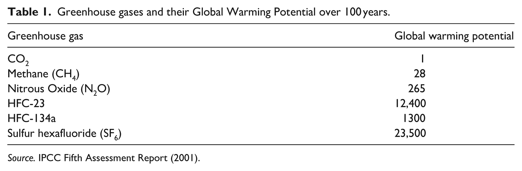
Source. IPCC Fifth Assessment Report (2001).
Results for the atmosphere
We begin with the longest time series of the CO2 concentrations in the atmosphere, and using nonparametric statistical tests, we show structural breaks, or “change points” in this long time series. We concentrate on the modern period in the analysis of Figure 1, running from the year 1502 to 2022, with results of the statistically identified structural breaks, or change points. Note specially the first change point is in 1780, showing a structural break in the distribution as a result of fossil fuel use, beginning with the Industrial Revolution.
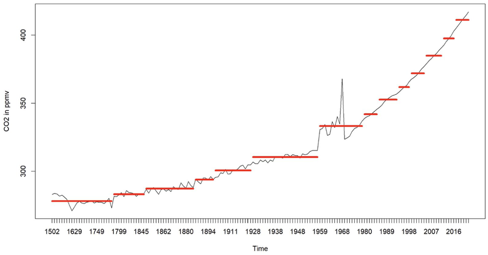
CO2 emissions in parts per million volume in the modern period starting in 1502, with the structure breaks identified by nonparametric tests.
From Figure 1, we can see that the statistical tests identify the following years as structural breaks, or change points: “1780”; “1846”; “1886”; “1900”; “1925”; “1958”; “1979”; “1985”; “1993”; “1998”; “2004”; “2011”’; “2016.”
As is customary, we can use exogenous information, such as historical events, that seem most likely to account for most of these structural breaks.
The modern era: The year 1500 and beyond
We note that from 1500, our statistical tests do not identify any breaks for 270 years. But we note the first structural break at 1780, showing the effects of the Industrial Revolution. The Industrial Age brought oil-using machines that slowly displaced coal-driven steam in factories, farms and railways beginning in the latter half of the 19th century, although coal continues to be used worldwide for power generation. The invention and mass production of the automobile and other engines relying on oil led to the exponential civilian use of oil through the 20th century. But that demand for oil was soon augmented by the armament industry, and the global military establishments. The exponential growth in demand for crude oil in the mid-20th century was no doubt behind the global exponential CO2 emissions shown in Figure 2, and is one of the key metrics of the Great Acceleration and its impact on the Earth system (Steffen et al., 2015).
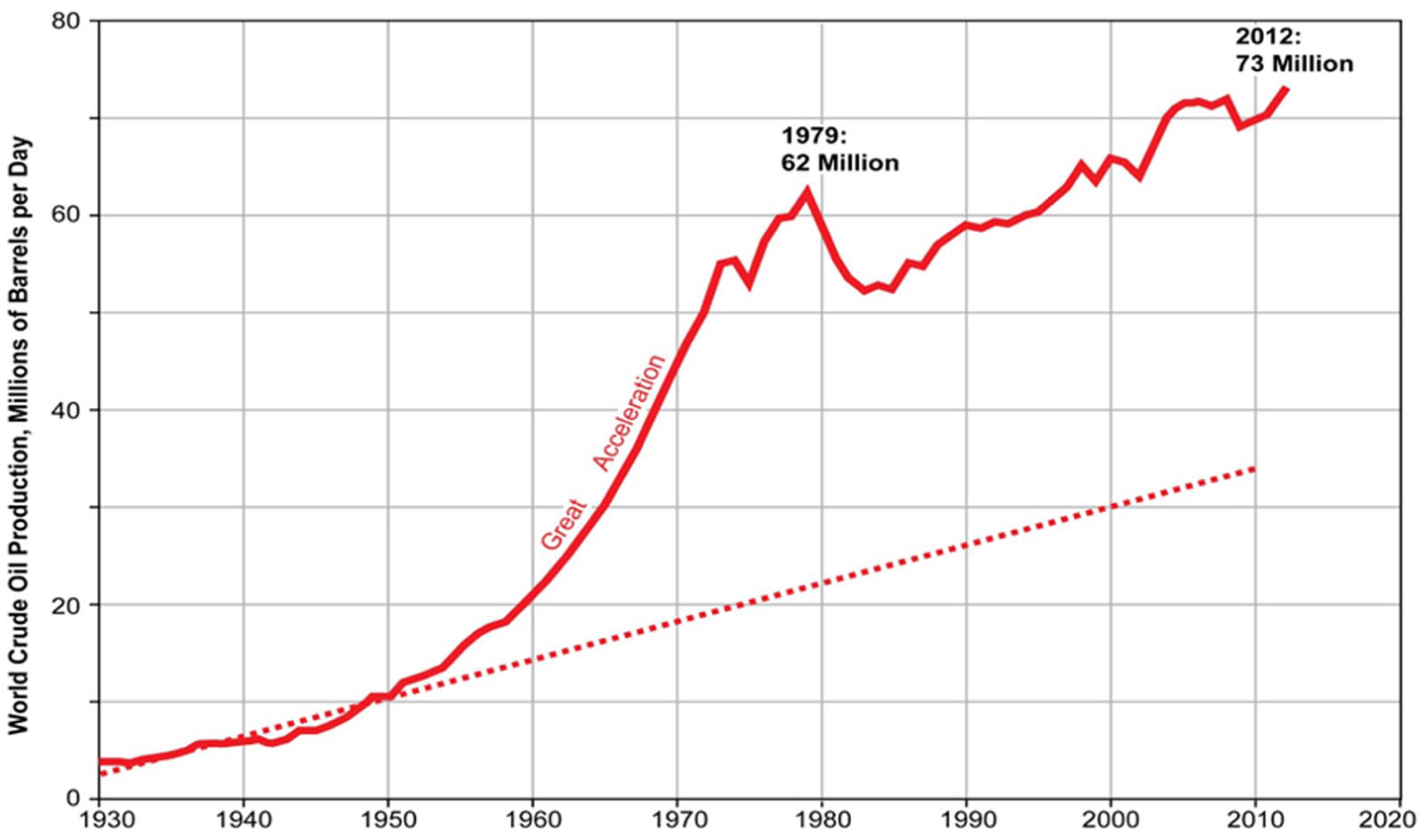
The exponential global growth of oil demand, needed by agriculture, industry, and the military.
We may now return to the structural breaks in the CO2 emissions identified in Figure 1, using two nonparametric tests, called BinSeg and PELT (for details see Appendix 1). Both tests identify roughly the same dates, with minor variations. Note however, that we are only considering the intersection of the two sets of structural breaks. These are breaks that are identified and confirmed by both tests.
The first structural break of 1780 is of course the impact of the Industrial Revolution. The other structural breaks can be plausibly associated with other exogenous information to account for the structural breaks, but the structural breaks that follow the year 1780 reflect increased “normal” civilian and military CO2 emissions, due to exponential growth in the consumption of coal, petroleum, and gas. This is shown in Table 2, using the dates identified by both tests. However, a word of caution: a structural break indicates a higher mean of the subperiod of CO2 emissions. This implies higher emissions from the previous subperiod. But Table 2 should not be interpreted as direct cause-and-effect, as in mechanical causes, but as being highly probable association of the impacts of petroleum-using inventions, or other historical “events” and their additional impacts on the growth of CO2 emissions. It is the exogenous information that seeks to explain and interpret these structural breaks in Table 2.
Structural breaks identified by “pelt” and “binseg” and inventions or historical events that increased the consumption of fossil fuels.
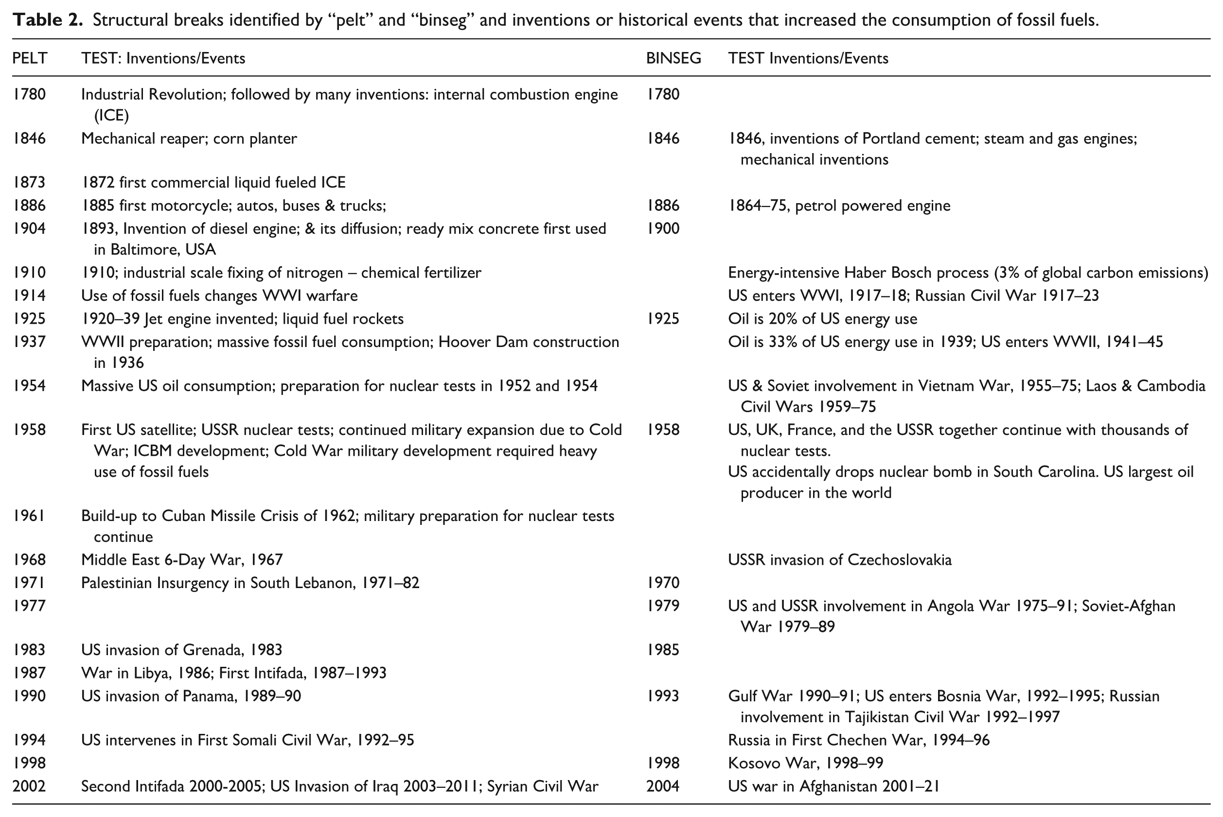
We see that the majority of those structural breaks, indicating a major change in the time series of CO2, are associated with the fruits of inventions such as the internal combustion engines and its uses in an increasing variety of mechanical inventions that are labor-saving and increase the productivity or output per unit of labor hour: for example mechanical reapers, corn planters, petroleum powered engines for motor cycles and automobiles, increased use of diesel (first developed from oil in 1893) in machines. This age of invention increased both food production as well as industrial production. The social costs of the use of fossil fuel were not known to humankind; the use of “cheap” fossil fuel energy, together with technological innovation turned out be the most important necessary conditions for the phenomenal growth of per capita income, output, and wealth in the developed or industrialized world. No doubt this was complemented by advances in hygiene and medical sciences, which then led to a dramatic rise in human populations.
Pari passu with industrial and agricultural development, fossil fuel changed the nature of war from World War I onward (for evidence see Gliech (2015)). The development of the jet engine in the 1920s (using fossil fuel of course) changed air transportation but it first transformed war once again (see Table 2). The “radial” expansion of industrial and commercial use of petroleum continued through population growth, and the cheapening of industrial goods, through productivity gains and technological improvements. But to this, one must superimpose, the new “structural” factor of war preparation and the military use of fossil fuels by all the major powers, which was later to include China.
The military preparation included nuclear bomb testing that spanned from 1944 onward, including the 1950s and the 1960s, when bombs were exploded both in the air, and underground as well as on islands, mostly in the Pacific. According to the Arms Control Association, at least eight countries have carried out a total of 2056 nuclear tests since 1945. Of those, 507 have been atmospheric explosions, which spread radioactive materials through the atmosphere. The United States has conducted just over half of all nuclear tests, with 1030 tests between 1945 and 1992. However, each test requires enormous preparation and use of fossil fuel energy for construction and testing, which leads to increased CO2 emissions in addition to that produced by the civilian populations of the world. But note that a nuclear explosion itself does not release CO2, except when followed by fires and burning of materials. But the preparation for each test requires enormous amounts of fossil fuel energy.
Each nuclear bomb test releases several radionuclides such as 137Cs, 90Sr, 239+240Pu, 241Am, and 131I. These nuclides end up in the atmosphere and the geosphere; they also ended up in living cells by way of the food chain. Following the successful testing of the first ever nuclear bomb on July 16, 1945, residents of New Mexico suffered radiation poisoning and sued the US government. A subsequent scientific reconstruction of the possible radiation damage to the population was published in National Cancer Institute (2020). The reconstruction was carried out by scientists and doctors at the US Center for Disease Control, at the request of the US government. But, of course, the definitive proof of death, destruction and radiation poisoning comes from the two nuclear bombs that were dropped on Hiroshima and Nagasaki in August 1945. Hence 1945 is a high watermark of the human impact on the Earth System; the fallout affected the atmosphere, the land and the marine environment.
One of the most representative examples is the isotope 14C produced in the upper atmosphere during nuclear tests, which then reached the marine environment, by means of the ocean–atmosphere gas exchange, or the biosphere through the process of photosynthesis. The increase in the thyroidal cancer incidence in many areas of the globe (strongly affected by the radioactive contamination with the 131I radionuclide) is the one among the worst consequences of nuclear testing. Eventually in 1963, the Limited Test Ban Treaty was passed; it led to a huge reduction in atmospheric explosions.
Military emissions are recognized as a very large component of global GHG emissions but reliable data on such emissions are difficult to find. The Paris Agreement of 2015, signed at COP21, has no specific requirement to report on direct emissions of defense departments of all countries. This is now being referred to as the “military emissions gap” (Climate Change Performance Index, 2024). The submission of data on total GHG emissions for military establishments is voluntary, and very little information has been reported to the IPCC. The major powers of the developed countries have not complied.
One estimate of global military emissions put it as 5.5% of all global CO2 emissions, which is more than the total annual emissions for the whole of Africa (Linsey Cottrell at Conflict and Environments Observatory). The US Department of Defense uses 93% of all US fossil fuel energy used by the government. The Union of Concerned Scientists (June 30, 2014) claimed that the US military consumes 100 million barrels of oil per year. Using the EPA calculator, 1 barrel of oil yields 426.10 kg of CO2 emissions. It follows that this method indicates that for 100 million barrels, the CO2 emissions must be 426.1 million MT of CO2. Crawford (2022) has used the Defence Logistics Agency data, and she concluded that the US Defence Depart used 122.4 million barrels of oil per year, which raises the estimate to 521.5 million MT of CO2 per year. In 2022 total US emissions were 6343 million MT of CO2 (EPA data). That would mean that annual military emissions would be between 6.7% and 8.2% per year for the US.
It should be noted that the above estimates of US military CO2 emissions are based on “normal” day-to-day operations of the US military, covering regular military exercises. Those estimates do not cover CO2 emissions when the US military is engaged in wars. A war outside the US can add more 100 million MT of oil per year. According to Reisch and Kretzmann (2008), the Iraq War (2003–2011), added 141 million metric tons of CO2 from March 2003 to March 2008. To quote them: “If the [Iraq] war was ranked as a country in terms of emissions, it would emit more CO2 each year than 139 of the world’s nations do annually.” (Reisch and Kretzmann, 2008).
Furthermore, while we suggest that the larger wars stand out in the structural breaks listed in Table 2, it is not possible to ascertain the CO2 impacts of the smaller US wars, such as (1) US occupation of Nicaragua 1912–33; (2) US occupation of Haiti 1915–34; (3) US occupation of the Dominican Republic 1916–34; (4) Bay of Pig invasion of Cuba 1961; and (5) continued supply of CO2 emitting military hardware to Israeli war efforts over the last 77 years.
The UK too has been involved in colonial and civil wars in southeast Asia and Africa over the last 50 years; France had its own colonial wars in Algeria and elsewhere; China has had wars over the south Pacific with Vietnam (1965–69), with the conquest of the Paracel islands (1974) as well as other minor skirmishes with India; and Russia has intervened militarily several times after 1990 in several of the former Soviet republics.
Hence the global military powers that are also states with nuclear weapons may have contributed massively to CO2 emissions not only through their military preparedness exercises and war games but also in actual wars involving deaths and destruction, in the past. Sadly, wars and proxy wars between rival military powers are continuing in the present. These continuing war emissions pose a major threat to the planet, both through additional CO2 emissions as well as land degradation.
Results for the oceans
The earth’s carbon is stored in four reservoirs: ocean, atmosphere, plants and soil, and fossil fuels. Carbon flows between each reservoir in an exchange called the carbon cycle, which has slow and fast components. Any change in the cycle that shifts carbon out of one reservoir puts more carbon in the other reservoirs. Changes that put carbon gases into the atmosphere result in warmer temperatures on Earth and also of the oceans. The oceans have been absorbing about 26% of the CO2 emissions; the oceans are also absorbing 90% of the heat generated on earth over the last 50 years, without which land temperatures would have been much higher. Their capacity to do so is not limitless, however, and cannot compensate for increased emissions.
NASA scientists have found that global mean sea level has risen 10.1 cm (3.98 inches) since 1992. Over the past 140 years, satellites and tide gauges together show that global sea level has risen 21–24 cm (8 –9 inches).
The absorption of CO2 has also led to the acidification of the oceans. The chemistry of acidification is well known. Dissolved CO2 combines with water to form carbonic acid (H2CO3) and increases the hydrogen ion (H+) concentration in the ocean, and thus decreases ocean pH, as follows:
The decrease in ocean pH is acidification, with serious implications for all marine life. Based on chemistry, we regressed pH on CO2. In an ideal world, it would be preferable to use the same time span, for the regression as the CO2 time series of 1502–2022. Unfortunately, such a long time series for ocean CO2 is not available. Fortunately, the shorter time series cannot result in any biases, as a matched shorter CO2 time series will not change the results of the measured ocean CO2, which rely on modern technology, which was not available to public agencies prior to 1985. Also note that a time series of 36 years (1985–2021) is long enough for statistical inference. The available data was from 1985 to 2021 and were obtained from the European Environment Agency (https://www.eea.europa.eu/en/analysis/indicators/ocean-acidification). Here are results of that regression (Table 3):
Regressing pH, with CO2 as the Independent variable.
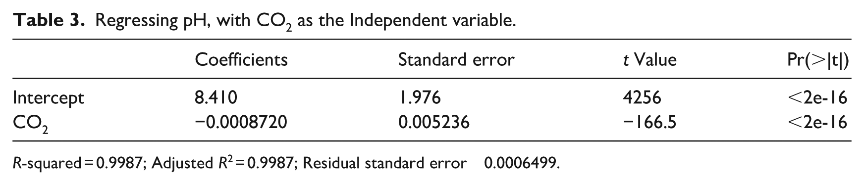
R-squared = 0.9987; Adjusted R2 = 0.9987; Residual standard error 0.0006499.
The regression is an extremely good fit and is justified by the chemistry equation stated above. Based on this model, if CO2 were zero, the average ocean pH predicted by this model would be 8.41. This agrees with the literature on ocean pH. Also, based on the regression model estimated above, we find that an increase of one particle of CO2 per million volume will produce a decrease in pH of −0.0008720. But ocean pH can vary from 8.0 to being as high as 12.5 in deep waters (Mottl, undated, Geochemical Society.)
Less alkaline water makes it harder for some species to form their shells, notably those of microscopic “sea butterflies” that form an important link in Arctic marine food webs. Rising ocean temperatures are causing a variety of problems, including loss of sea ice, more frequent, intense storms, and marine heat waves that can kill off millions of animals.
Results of impacts on land
In the search for increased food production, or for increased profits, large areas of land have been stripped of forests and wetlands; and the oceans have been fished by factory-fishing ships all over the globe. The consequence has been continued loss of biodiversity. The Living Planet Index (LPI) – which tracks populations of mammals, birds, fish, reptiles, and amphibians – reveals an average 69% decrease in monitored wildlife populations since 1970. The 2022 LPI analyzed almost 32,000 species populations. It provides the most comprehensive measure of how these species are responding to pressures in their environment.
The information on the continental distribution of biodiversity loss is given in Table 4.
Continental distribution of the loss of biodiversity.
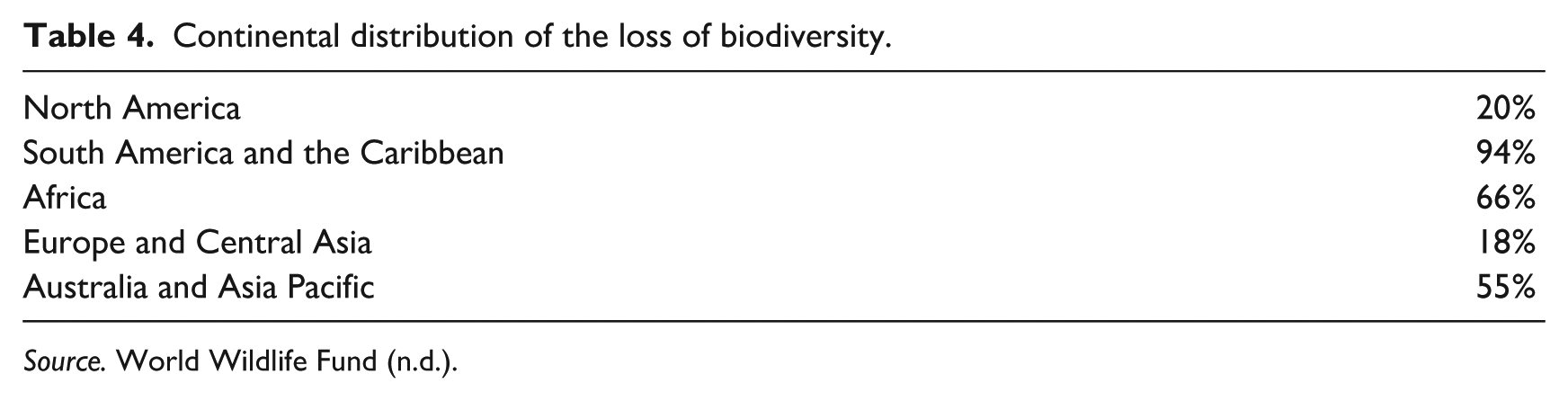
Source. World Wildlife Fund (n.d.).
The International Union for the Conservation of Nature (IUCN) has a “Red List” of endangered species. It now includes 147,517 species, of which 41,459 are threatened with extinction.
Today’s Red List update highlights the fragility of nature’s wonders, such as the unique spectacle of monarch butterflies migrating across thousands of kilometres,” said Dr Bruno Oberle, IUCN Director General. “To preserve the rich diversity of nature we need effective, fairly governed protected and conserved areas, alongside decisive action to tackle climate change and restore ecosystems. In turn, conserving biodiversity supports communities by providing essential services such as food, water and sustainable jobs.” (IUCN, 2025)
According to the IUCN, the endangered migratory monarch butterfly is a subspecies of the monarch butterfly (Danaus plexippus). The native population, known for its migrations from Mexico and California in the winter to summer breeding grounds throughout the United States and Canada, has shrunk by between 22% and 72% over the past decade. Legal and illegal logging and deforestation to make space for agriculture and urban development has already destroyed substantial areas of the butterflies’ winter shelter, while pesticides and herbicides used in intensive agriculture across the range kill butterflies and milkweed, the host plant that the larvae of the monarch butterfly feed on.
We found time series data on trends in the abundance of butterflies in the UK: 1976 to 2022. This indicator includes individual measures for 51 species of butterflies; the UK “all-species” butterflies index, however, only includes 50 trends. This is because an aggregate trend is used for small skipper (Thymelicus lineola) and Essex skipper (Thymelicus sylvestris); these 2 species have been combined due to historical difficulties with distinguishing between them in the field. The index is taken as 100 in 1976 and has fallen to 52 in year 2022. Figure 3 attempts to discern structural breaks in this population. We used BinSeg to look for 3 change points. This struggling population shows the following three change points: years 1988, 1997 and 2017. We need to check with lepidopterists if this population can recover. Repeated structural breaks in a population are indicative of extreme stress. Some animal and insect populations may be subject to predator-prey cycles, but the rapid decline in this population is cause for concern. The recovery of this population might require cessation of the use of farm and lawn pesticides, and a restoration of lost habitats – a tall order indeed.
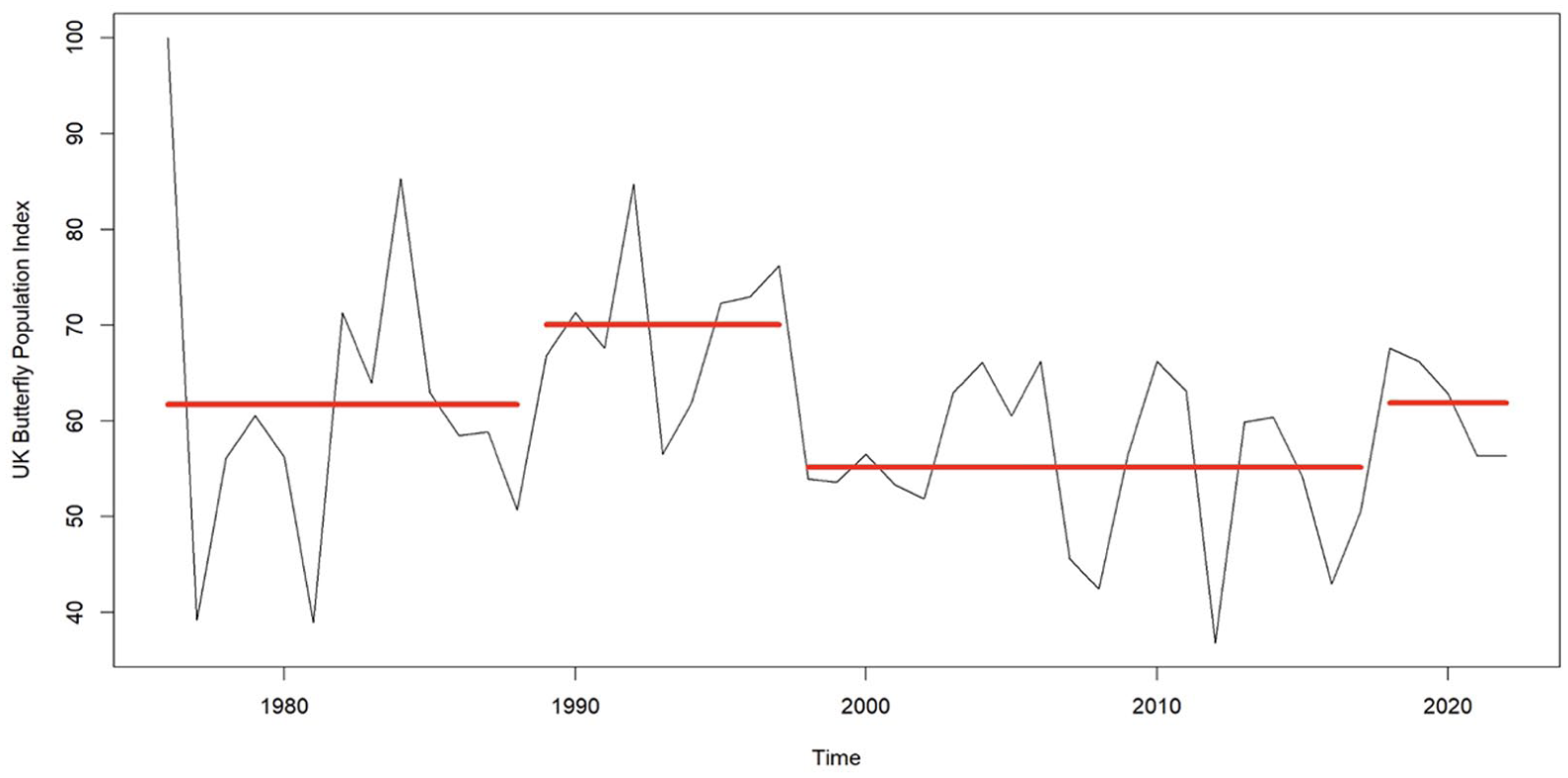
The changing and collapsing distribution of UK butterfly population unsmoothed index (1976 = 100).
There is further bad news from a newly published study in the UK. In recent years, concerns have been raised over earthworm populations, which have fallen by a third in the past 25 years. A new statistical study by Ball (2022) that monitors flying insects in the UK, found a 58% decline in insect population between 2004 and 2021.
Results for impacts on the global temperature
The Land-Ocean Temperature Index is a measure of how global average temperatures have changed over long periods of time. This is a planetary index, integrating the human impacts on land, air, and on the oceans. It also includes land degradation through habit loss, using fossil fuels. But we should also consider the biodiversity index for land degradation as additional evidence.
In Figure 4 we present land-ocean temperature index, which shows global warming from 1880 onward. It will be seen that in this early period, the average is negative. In 1930, it first turns to zero but then briefly turns negative again. Of course, this global average is subject to many influences, including solar variability. In Figure 5, we analyze the percentage of variation of the land-ocean temperature index, using PELT to identify structural breaks, in the time series starting in 1880.
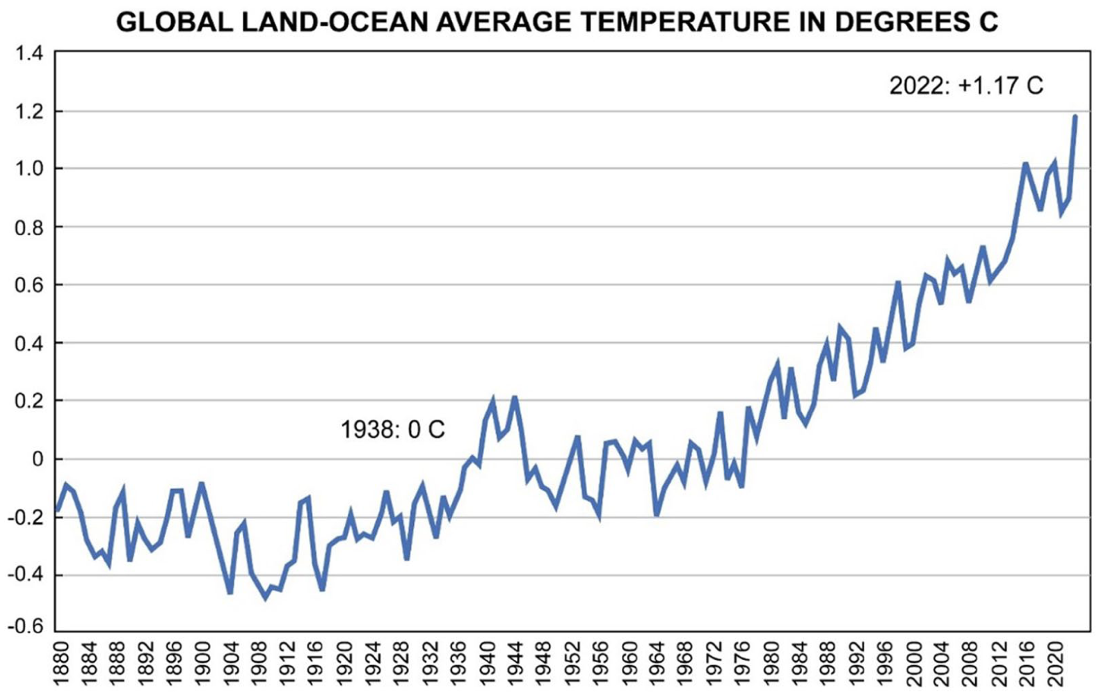
Global Land-Ocean average temperature index in Degrees C.
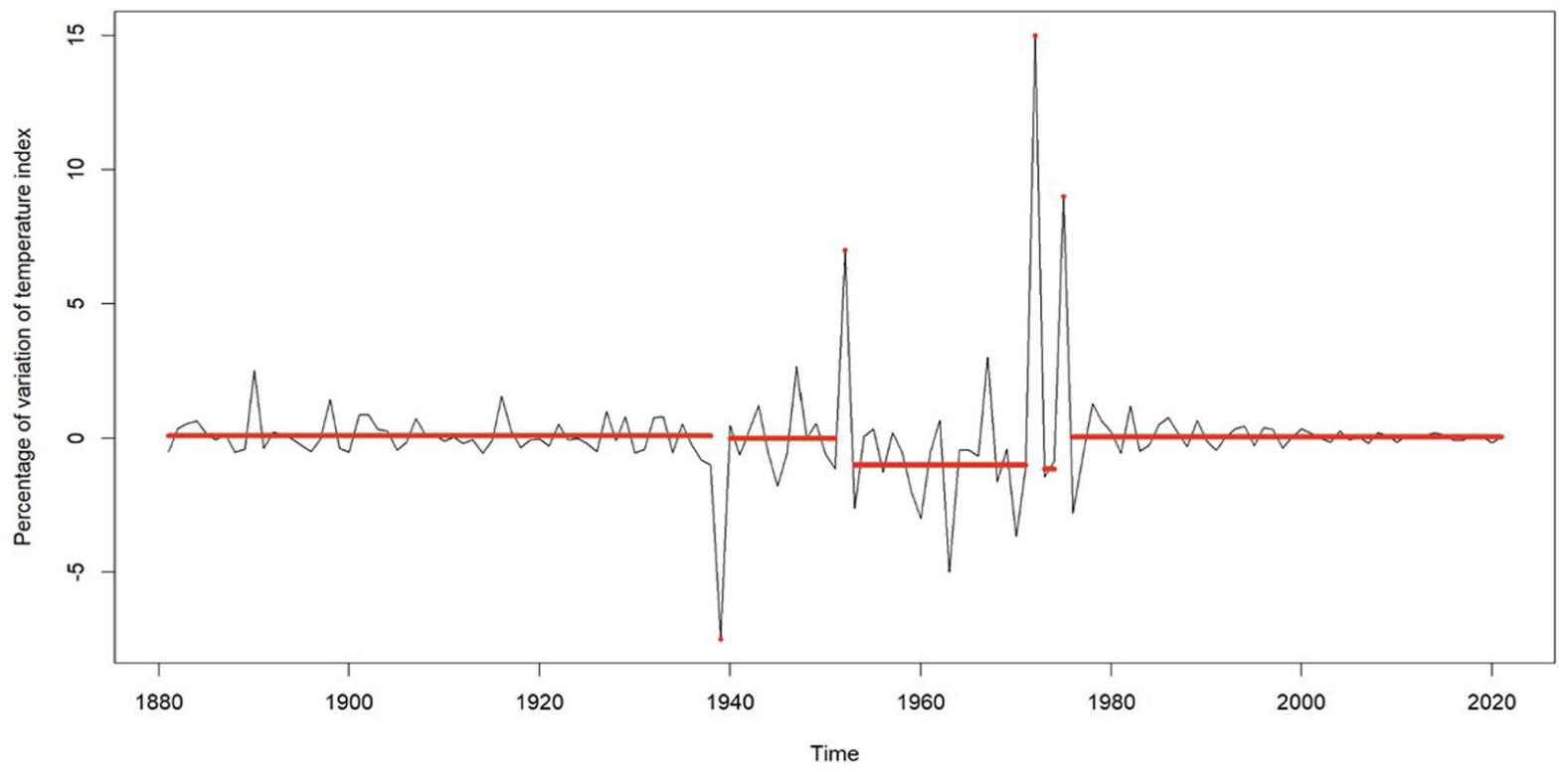
Variation of the Land-Ocean Temperature Index, with structural breaks.
The statistical exercise identified the following years as the structural breaks: 1937; 1939; 1951; 1952; 1971; 1972; 1974 and 1975. Geoscience researchers demarcate recent geological “epochs” over the last 2.6 million years (the Quaternary Period) based on a geoclimatic referent, although most are marked by mass extinctions. Consistent with this practice, the beginning of the Anthropocene epoch should be marked by a geoclimatic referent. One such referent is when the global average temperature turned from negative to zero (see Figure 4) in 1938 and 1939, but that could be attributed to solar variability (National Research Council 2012), leading to statistical fluctuations. The next reliable structural breaks are in 1951 and 1952, which is consistent with the Anthropocene Working Group (AWG) proposal for a Global boundary Stratotype Section and Point (GSSP) in 1952 (McCarthy et al., 2025; Waters et al., 2024a, 2024b, 2024c). The structural breaks later in the 1970s are indicative of the continued acceleration of the average global temperature, no doubt due to increased GHG emissions until the demand for crude oil flattened during the OPEC Crisis.
Comparing our results with those of the AWG
Geological time is divided into “eons,” which are then subdivided into “eras,” “periods,” “epochs,” and finally into “ages.” Each of these units of geologic time is defined at its base at a particular point in a stratigraphic section somewhere on the planet where a major global change is recorded – the equivalent system to define each period, series to define each epoch and stage to define each age. For example, the Quaternary Period is defined by the accompanying “rock-stratigraphic system” near the Sicilian city of Gela, and this Global boundary Stratotype Section and Point (GSSP) also defines the beginning of the Pleistocene Epoch and the Gelasian Age (the age is always named after the site where the stage is defined). The Holocene Epoch is divided into (a) the Greenlandian age with its GSSP in a core from the Greenland Ice Sheet also defining the boundary between the Pleistocene and Holocene Epochs; (Walker et al., 2012), (b) the Northgrippian Age, and (c) the Meghalayan Age, which is defined by a “golden spike” in mineral deposits from Mawmluh Cave, in India (Cohen et al., 2020; Walker et al., 2018).
The International Chronostratigraphic Chart (IUGS, 2023) shows the complete geological record of the history of the earth. The Anthropocene Working Group proposed that a third epoch of the Quaternary Period began in the mid-20th century (Waters et al., 2024a) when the Earth System rapidly departed from Holocene norms due to the Great Acceleration (McNeill and Engelke, 2016), as proposed by atmospheric chemist Paul Crutzen (Crutzen and Stoermer, 2000). High concentrations of fly ash and blooms of microscopic algae that thrive in high CO2 environments record the rapid post-WWII increase in fossil fuel combustion, cement production and deforestation in the early 1950s, and other microfossils and the acid rain that accompanied industrial activity prior to enactment of Clean Air legislation, are evident in the seasonally layered sediment record from Crawford Lake, Ontario, Canada (Figure 6).
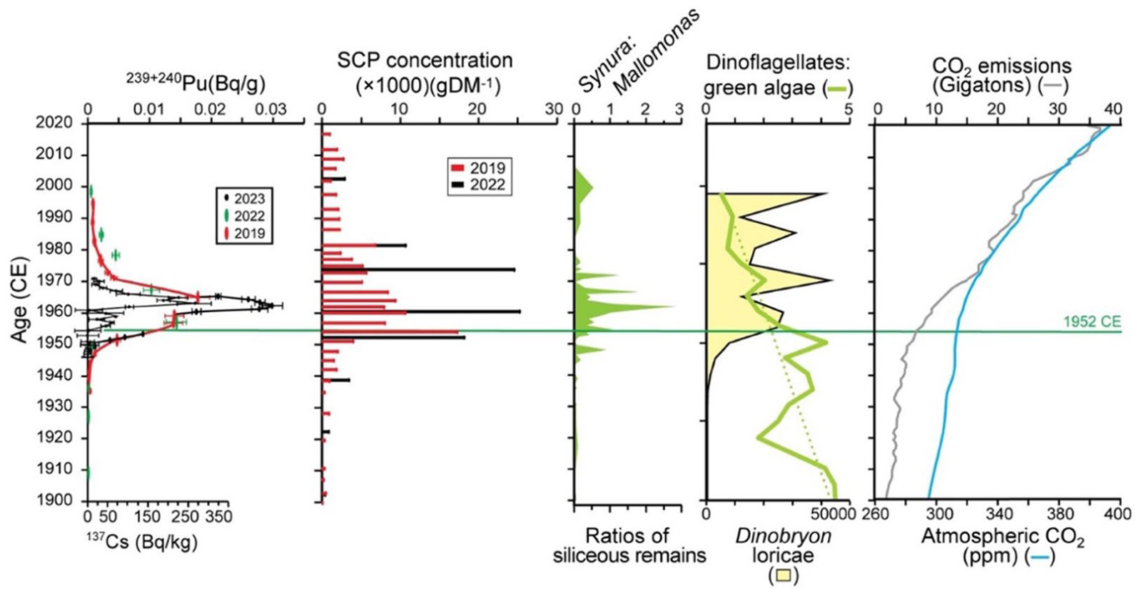
Summary of proxies of the Great Acceleration and the Nuclear Era measured in sediment cores collected in 2019, 2022 and 2023 from Crawford Lake, with the rapid increase in plutonium associated with thermonuclear weapons (H-bombs) defining the base.
The markers of human industry and land use change (i.e. the Great Acceleration) are regional and slightly diachronous through the mid-20th century – considerably earlier in western Europe and North America than in East Asia. The marker preserved in geologic strata that was chosen to define the beginning of the Anthropocene is thermonuclear weapons fallout, specifically isotopes of plutonium, 239+240Pu (239 + 240) produced during nuclear fission. The synchroneity of this anthropogenic marker is evident at five sites considered by the AWG in addition to Crawford Lake, shown in Figure 6. A sharp increase in plutonium associated with thermonuclear explosions (H-bombs) was measured in the dark-colored sediment layer deposited in Crawford Lake during the fall of 1952 (McCarthy et al., 2025) providing a nominal age to mark the beginning of the Anthropocene epoch: of 7:15 AM on Nov. 1, 1952 in the Marshall Islands, the moment the first H-bomb (Ivy Mike) was detonated in the Pacific Proving Grounds, as shown in Figures 6 and 7.
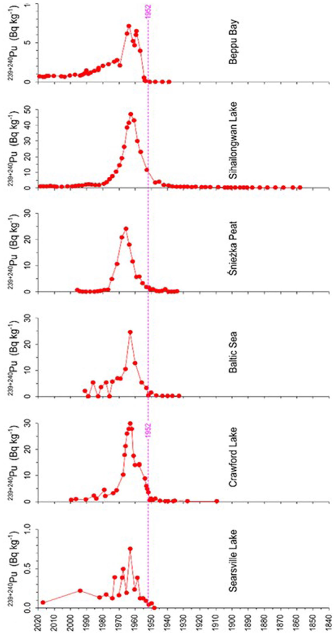
Measured 239+240Pu in sediment cores from Searsville Lake (USA), Crawford Lake (Canada), the Baltic Sea, Sniezka Peat (Poland), Shihailongwan Lake (China), and Beppu Bay (Japan) showing the globally synchronous increase in the early 1950s and a peak in the mid-1960s, when the Limited Test Ban Treaty was ratified. From Waters et al. (2024b).
Unprecedented public interest in bureaucratic decisions of geologic organizations ensued following the announcement that the annually laminated sediments from Crawford Lake (Figure 7) were selected as the proposed GSSP to define the Anthropocene epoch. This presumably reflects the realization that humans have, in fact, impacted the Earth System, resulting in what is typically simplified in the popular media as the “Climate Crisis” (Oreskes, 2024). The formal proposal submitted October 31, 2023 to the Subcommission on Quaternary Stratigraphy summarized evidence for an altered planet from Crawford Lake and three Standard Auxiliary Boundary Stratotypes from a lake in China, a marine harbor in Japan, and a peat bog in Poland (Waters et al., 2024a, 2024b, 2024c).
In March 2024, the media and scientific publications reported that the Subcommission on Quaternary Stratigraphy voted against adding the Anthropocene to the Geologic Time Scale and they ignored the proposal to add a Crawfordian age (whether as the fourth age of the Holocene or the first age of an Anthropocene epoch). Its parent body, the IUGS quickly ratified this vote, despite its legitimacy being contested on procedural grounds. A reporter from the journal Science entitled his article: “The Anthropocene is dead. Long live the Anthropocene” (Voosen, 2024). An editorial in the journal Nature highlights the importance of formally recognizing the Anthropocene, concluding “The absence of an agreed marker and a specific start date should not detract from the reality of a discernible human fingerprint on Earth systems” (Editorial, Nature vol, 627, p. 466, March 21, 2024).
There are two key questions remaining: (1) are we still living in a Holocene world and (2) is the date Nov. 1, 1952 consistent with geological evidence of an altered Earth System? To answer the first, the current planetary conditions have no analog through the Quaternary Period; in fact, the closest analogs for conditions predicted before the end of this century are from 3.5 million years ago, long before evolution of the genus Homo. As early as 2003, Nobel laureate Paul Crutzen wrote that that “the Earth System has recently moved well outside the range of natural variability exhibited over at least the last half million years” (Crutzen and Steffen, 2003: 258). Ignoring the data showing this to protect “the sanctity of the field of geology . . . from initiatives that some see as political” (Geological Society of America, 2024) is not in keeping with the scientific method. Even though the Geologic Time Scale still has us officially in the Holocene Epoch, we are clearly not living in a Holocene world.
To answer the second, ours is not the only statistical study to identify shifts consistent with the AWG proposal for a golden spike to define an Anthropocene epoch beginning around 1952. In a recent statistical paper, On et al. (2024) attempt to identify changes in the geologic record based on a multilevel Bayesian change point model, utilizing 9 of the 12 GSSP candidate sites. Their meta-analysis concluded that the greatest shift in the Earth System was in year 1953, within a confidence interval of 1952.5–1954.5. This is consistent with the GSSP proposed in the organic sediments deposited from fall 1952 through spring 1953 at Crawford Lake (McCarthy et al., 2023, 2025). On et al. (2024) employ a continuous piecewise linear regression model with a single change point, indicating the break point in the line. The assumption is that the change point can be identified at the point where a zero slope abruptly turns positive, and that there is only one such critical change point. The meta-analysis also assumes that the change point at the population level follows a truncated t-distribution. The final results are highly dependent on a host of assumptions, including the linearity assumptions of the regression models of the 9 sample models as well as the population (or “meta”) model.
Kuwae et al. (2024) carried out a much larger study of what they call “human fingerprints” in the geological strata from 388 proxy records taken from 137 sites located in geological strata of the Antarctica, Arctic, East Asia, Europe, North America, Oceania, and other regions. To determine statistically the change from Holocene to Anthropocene conditions, they seek to find “change points.” They perform two statistical analyses: a change-point analysis to detect a significant change point in the time series using changes in the mean of all time-series data, and a break-point analysis to segregate the trends in time-series data using two consecutive linear-regression relationships and show the multiple change points in the time series. They allow for 5 break points, where the change point is determined by “change point” commands available in the statistical package called R. To guard against the error of selecting too many change points, they use the (customary) Modified Bayesian Information Criteria (MBIC) as a penalty, which is what we use too in our nonparametric tests BinSeg and PELT. Their change point was centered on 1952, within the confidence interval of plus or minus 3 years, that is, from 1949 to 1955. The peak of anthropogenic fingerprints was detected in 1953, including. . . “increases in 239+240Pu, 236U/238U, and 137Cs, as well as the first appearance of persistent organic compounds such as polychlorinated biphenyls (PCBs), DDT, hexachlorocyclohexanes (HCHs), and PAHs,” (Kuwae et al., 2024: 5).
The sharp increase in radioactive fallout measured by United Nations Scientific Committee on the Effects of Atomic Radiation (UNSCEAR, 2000) and the sharp increase in 239+240Pu measured in sediments deposited between the fall of 1952 and spring of 1953 makes the detonation of the first H-bomb a useful nominal moment in time to define the beginning of a new epoch. The sharp increase in this anthropogenic isotope coincides with the other markers of the Great Acceleration not only at Crawford Lake but also at other locations.
Conclusion
Our paper relies of the statistical analysis of time series, based on nonparametric tests, which determine the structural breaks, an approach that is model free and hence is more general. Then using parametric modeling, we demonstrated that the three main greenhouse gases, CO2, methane and nitrous oxide were cointegrated, and were all themselves the result of the production and use of fossil fuels. Given this co-dependence, it was legitimate in the rest of the section to rely on CO2. We find that apart from the continuous (radial) growth of civilian use of fossil fuels, the large additional military use of fossil fuels beginning before WWI and all other wars, small, and large, led to the exponential growth of GHGs and exponentially rising global temperatures during the mid-20th century. It has been estimated that the global military use of fossil fuel has added 5.5% of the total global GHG emissions. This additional military emissions may still be an underestimate because reporting of military emissions is still voluntary.
The structural break in the CO2 in the atmosphere began with the start of the Industrial Revolution around 1750s but the accumulation and statistical structural break marking the effects of the Industrial Revolution occurs in 1780, when human reliance on fossil fuels began. The entire course of human civilization is dependent on the cheap energy that fossil fuels made possible. Indeed, we argue that fossil fuel use is the dominant factor in explaining technological and economic development of Homo sapiens, with the emergence of a food surplus, labor specialization, and social organization that permitted population growth, increasing but unequal prosperity, and rising living standards based on human made machines that relied on energy from fossil fuels. Even the emergence of nuclear bombs and other nuclear uses required fossil fuels as the necessary condition.
The use of fossil fuel radically transformed our terrestrial home: mechanized agriculture led to a rapid deforestation and loss of habitat for wildlife and an alarming loss of biodiversity globally. The accumulation of CO2 in the atmosphere also impacted the oceans, with growing acidification of the oceans and a rise in its average temperature, with mostly negative impacts on marine life.
Although Paul Critzen first proposed the Industrial Revolution as the possible start of a new epoch that ended the Holocene, he was careful not to put a date to it, recognizing that further research was needed and he eventually accepted the mid-20th century Great Acceleration as the most distinct difference between the Holocene and a human-altered Earth system. To follow GSSP protocol, we need to observe clear scientific criteria for dating the end of one epoch and the start of another. A candidate “date” for the start of the Anthropocene must be grounded on a criterion of scientific validity based on observation and measurable detection supporting some seismic change experienced worldwide, based on markers preserved across the world in the geologic record. Furthermore, it should stand up to global scrutiny and can also be validated by alternative scientific observations and measurable quantities.
Our statistical quest is to seek de novo, a final statistical test that represents an integrated planetary index of the effects of human activity. That index is the global average temperature. We were again able to find structural breaks in the variation of the global average temperature time series. This analysis unambiguously points to 1952 as the proposed beginning of the Anthropocene, consistent with the AWG proposal (McCarthy et al., 2025; Waters et al., 2024a, 2024b, 2024c). This date for a dramatic shift in the Earth System was supported by statistical analysis of multiple markers by On et al. (2024) and Kuwae et al. (2024), but our result is model free, that is, not based on the prior imposition of a linear model on the data. This reckless disregard of the consequences of our modern industrial culture has increasingly strained the Earth System and now threatens biodiversity as well as the future of Homo sapiens. In sum, we have statistically analyzed the serious anthropogenic impacts resulting in the accumulation of greenhouse gases in the atmosphere and its effects on the global average temperature and associated environmental conditions, such as sea level. Since the proposed GSSP in the sediments of Crawford Lake is supported by various statistical analyses of markers of the planetary system, adding the Anthropocene epoch to the Geologic Time Scale (and, by definition, mark the end of the Holocene Epoch) would draw increased attention to environmental conditions that have no recent analogs.
Footnotes
Appendix 1: Non-parametric tests used in this paper to identify structural breaks in time series data
We use two tests to identify structural breaks, or change points in a time series: Binary Segmentation (or BinSeg), (see Scott and Knott, 1974) which is available in most statistical packages, and Pruned Exact Linear Time (PELT), developed and published by Killick et al. (2012). This test is available in R, which we used.
Appendix 2: On cointegration test for Co 2,methane (Ch4) and nitrous oxide (No 2 )
The text of this paper argues how the three gases “move together,” which is a form of linear co-dependence. Such variables are said to be “cointegrated,” if proven statistically. We already know from chemistry that the three gases originate from the production and use of fossil fuel energy. We therefore expect structural breaks in the 3 time series of the gases although of course they will not be identical.
There are statistical tests for cointegration, but when there are structural breaks, the tests become more difficult. Gregory and Hansen (1996) extended cointegration test to allow for one structural break; Hatemi-J (2008) extended it to allow for 2 structural breaks; and Maki (2012) extended his cointegration test to allow for up to 5 structural breaks. In this Appendix, we restrict our research for cointegration by first finding 5 structural breaks in our three variables. Here are our 5 best breaks in Table 5:
Our Null hypothesis is there is NO cointegration; that is, in the linear equation:
That is the cointegrating vector [a b c] does not exist.
Accordingly, we consider three model specifications to test for cointegration in the equation
Model 1: Level shift with trend:
Model 2: Level shift only:
Model 3: Regime shift only:
In Table 6, we report the Maki test statistic and the corresponding critical value.
Assume that incorporating 5 structural breaks in the three time series is representative of the larger number of structural breaks we identified using nonparametric methods in the longer CO2 time series. If that assumption is valid, then we can reject the null hypothesis of NO cointegration. The cointegration relationship give us the following expression:
With an R2 = 0.9916
So in fact, equation (A2) clearly establishes the linear dependence between the three variables, with a high degree of confidence.
Acknowledgements
The effort to identify a potential “golden spike” to define the Anthropocene as a geologic epoch owes much to collaborative efforts of the Anthropocene Working Group since its inception in 2009. We appreciate the assistance of M. Lozon, Brock University, with drafting some of the figures.

Funding
The authors received no financial support for the research, authorship, and/or publication of this article.
Declaration of conflicting interests
The authors declared no potential conflicts of interest with respect to the research, authorship, and/or publication of this article.