Short-lived persuasion from campaign rallies: Evidence from the 2016 U.S. presidential election

Introduction

Political campaigns are a central feature of electoral competition, and a large literature on political science and economics studies how campaign input shapes electoral outcomes and voter behavior. Researchers have examined the role of campaign contributions (Fremeth et al., 2013; Gordon et al., 2007; Snyder, 1990) and campaign spending (Gerber, 1998, 2004); the effects of media exposure measured through newspaper consumption (Gerber et al., 2009) or endorsements (Chiang and Knight, 2011); momentum in sequential elections (Knight and Schiff, 2010); the role of information in voter behavior and the allocation of campaign resources (Casey, 2015); and, more broadly, how office-seeking candidates should optimally deploy campaign effort (Stromberg, 2008). A recurring theme in this literature is that persuasion in high-salience general elections is difficult to achieve on average, consistent with “minimal effects” evidence from field experiments on campaign contact (Kalla and Broockman, 2018). Still, large in-person rallies remain a staple of campaign strategy, combining a candidate’s direct communication with voters and the potential for substantial local earned-media spillovers (Chiang and Knight, 2011; DellaVigna and Kaplan, 2007). ¹

This gap is partly due to identification challenges. A long political science literature studies candidate visits and campaign events using electoral returns, with mixed findings: some studies report meaningful gains from visits (Althaus et al., 2002; Heersink and Peterson, 2017); others find small, conditional, or null effects (Devine, 2018); and Heersink et al. (2021) find that campaign rallies can mobilize voters while also counter-mobilizing opponents. A central difficulty is that candidates choose where and when to appear strategically, making simple comparisons confounded by targeting and time-varying local political conditions (Stromberg, 2008). One rare exception is experimental evidence that randomizes (parts of) a candidate’s travel schedule (Shaw and Gimpel, 2012), underscoring how hard it is to obtain clean variation in rally exposure.

This paper asks whether, and how, campaign rallies shift voters’ preferences over both candidates and policies. I study the 2016 U.S. presidential election by combining individual-level data from the Cooperative Congressional Election Study (CCES) with the 2016 Presidential Campaign Tracker assembled by FairVote.org (2016), which records the timing and location of campaign events. ² The key empirical leverage comes from interview timing: within the same county, some CCES respondents are interviewed shortly before a rally occurs, while others are interviewed shortly after. I exploit this within-county variation, together with cross-county variation in where rallies take place, to estimate the effects of rallies using an event-study design that compares respondents interviewed just before and just after a rally within narrow event windows. Because exposure is defined at the county-level, this design identifies intent-to-treat effects of local rally occurrence (not individual attendance), capturing the combined influence of the rally itself and its local information environment.

Three patterns stand out. First, Hillary Clinton rallies generate a positive but short-lived increase in stated preference for Clinton: the effect appears immediately after the rally and fades after 5 days. Second, Donald Trump rallies produce heterogeneous short-run effects: in urban counties, preference for Trump declines significantly about 5–6 days after the rally, while in suburban counties it rises significantly and persists for roughly 1 week. In magnitude terms, the average post-rally effect is about 2 percentage points decrease in urban counties and 5 to 6 points increase in suburban counties. Third, I find no evidence of pre-trends in the days leading up to rallies for either candidate, supporting the interpretation that the post-rally dynamics reflect changes occurring after the event rather than differential trends already underway.

The paper makes three main contributions. First, it provides new quasi-experimental evidence on a prominent campaign input—rallies—in a setting where persuasion is often thought to be limited on average (Kalla and Broockman, 2018), and it does so for both major-party candidates in a high-stakes general election. Second, it shows that rally effects are sharply context-dependent: pooling across counties masks substantial heterogeneity in the direction and magnitude of responses, consistent with the idea that campaign messages can persuade some electorates while generating backlash in others. Third, it brings policy preferences into the analysis. In an exploratory analysis I also show that issue-position effects are limited, but Clinton rallies in suburban counties are associated with a modest leftward shift in a broad ideology index, whereas Trump rallies show little systematic evidence of shifting policy attitudes.

After documenting the dynamic responses, I estimate average effects. In the preferred specification, Clinton rallies increase the probability that a respondent prefers Clinton by 1.9 percentage points (and by 4.7–7.6 points in alternative fixed-effects specifications). Pooling all counties, Trump rallies are associated with a 1.6 percentage-point decline in stated support on average (statistically insignificant at conventional levels). This pooled estimate masks substantial heterogeneity. In urban counties, Trump rallies decrease the probability of preferring Trump by about 1.9–2.8 percentage points, while in suburban counties they increase it by about 5.4–6.5 percentage points; these two effects are statistically different. In contrast, I find no evidence that Clinton rallies have systematically different average effects across urban and suburban counties.

Finally, the paper studies policy preferences. Table 2 shows that issue-position effects are generally small and often statistically indistinguishable from zero. For Trump rallies, I find little evidence of systematic changes in policy attitudes in either urban or suburban counties, with the exception of a modest movement on crime in urban counties. For Clinton rallies, policy responses in urban counties are also small, but in suburban counties Clinton rallies are associated with a modest leftward shift in summary ideology measures (both the simple-average index and the Anderson index).

Data

Results

Event-study design and dynamic effects

Empirical approach

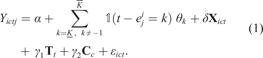
I estimate the dynamic effects of rallies using an event-study design, following Sandler and Sandler (2014) and in the spirit of Sun and Abraham (2020). The baseline specification is:

Y ictj = α + ∑ k = K ̲ , k ≠ − 1 K ¯ 1 ( t − e j i = k ) θ k + δ X ict + γ 1 T t + γ 2 C c + ε ict .

(1)

The outcome Y _ictj is a binary indicator equal to one if respondent i interviewed on date t reports preferring the focal candidate (Trump or Clinton) over any other option. ³ The vector X _ict includes basic respondent characteristics (age, gender, race, born-again Christian status, education, and income). I include county fixed effects C _c and survey-date fixed effects T _t to absorb persistent county differences and common time shocks. Standard errors are clustered at the county-level, to allow arbitrary correlation in unobserved shocks within counties over time. ⁴

Event time is measured relative to the date of the jth rally in respondent i’s county, denoted e j i , with k = −1 as the omitted category. I estimate (1) using a symmetric window around each rally (my baseline uses 15 days before and after). When a county hosts multiple rallies by the same candidate, I implement a stacked event-study as detailed in Appendix B. ⁵

Identification relies on two assumptions. First, within a county, the timing of CCES interviews is unrelated to campaign decisions about when to hold rallies. ⁶ Second, within a narrow window around a rally, the rally date is not systematically driven by short-run changes in local political conditions (e.g., campaigns do not reschedule rallies in response to day-to-day shifts in support).

The empirical strategy exploits the fine timing of rallies: I compare respondents interviewed shortly before versus shortly after a rally in the same county. With county and survey-date fixed effects, identification comes from within-county changes in outcomes at the rally date relative to other counties interviewed on the same days. I assess the plausibility of the design by estimating event-time coefficients prior to rallies and showing lack of evidence supporting outcome pre-trends. ⁷

Exposure is defined at the county-level: a respondent is classified as exposed if a rally has occurred in their county by the interview date. ⁸ This is an intent-to-treat measure of local exposure to campaign activity (not individual attendance). The key remaining identifying assumption is that, within the event window, there are no county-specific shocks to voter preferences that coincide with rally timing; the absence of pre-trends in Section 3.1 provides supporting evidence.

The dynamic effects of rallies on voters’ preference for Trump and Clinton

Figure 2 displays the dynamics effects of Trump and Clinton rallies, respectively, following the specification of equation (1). The sample used in the main specification is restricted to 15 days around rallies’ dates. Pre-treatment coefficients are generally small and always statistically indistinguishable from zero at any common significance level. The null hypothesis that all pre-treatment coefficients are jointly equal to zero also fails to be rejected, with the F-Tests yielding p-values of 0.817 for Trump and 0.169 for Clinton. Robustness checks with a window of 30 days are presented in section 4.OPEN IN VIEWER

Figure 2.

Effect of rallies on preferences over candidates (15-day window). This figure shows the coefficients retrieved from estimating equation (1). Figures 2(a) and 2(b) estimate the effects of Trump rallies in the voters’ preference for Trump and the effects of Clinton rallies in voters’ preference for Clinton, respectively. Robust standard errors are clustered at the county-level.

Two patterns are immediate. First, Figure 2 shows little evidence of pre-trends in the days leading up to rallies for either candidate, supporting the interpretation that the post-rally dynamics reflect changes occurring after the event rather than differential trends already underway. Second, the post-rally responses are short-lived. For Trump, the main movement is a temporary decline in stated support that appears about 5–6 days after the rally and then dissipates; during the first 4 days after the rally, estimates are close to zero. This pooled pattern averages over offsetting spatial effects: as shown in section 3.3, the post-rally decline is driven by urban counties, while suburban counties exhibit an immediate increase in Trump support. For Clinton, the response is quicker: support increases immediately after rallies, is statistically significant within 1–2 days, peaks around 3–4 days, and then fades back toward zero roughly 5 days after the event.

These qualitative patterns are robust to alternative event-window choices (e.g., 30 days), endpoint binning (Schmidheiny and Siegloch, 2020), and reasonable changes in the binning scheme (detailed in section E).

Average effects

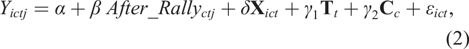
To summarize the event-study dynamics with a single estimate, I replace the event-time indicators in equation (1) with an indicator for being interviewed after a rally. Specifically, After_Rally _ctj equals one if a rally in respondent i’s county occurred in the previous 14 days, and zero otherwise. The estimating equation is:

Y ictj = α + β A f t e r _ R a l l y ctj + δ X ict + γ 1 T t + γ 2 C c + ε ict ,

(2)

with standard errors clustered at the county-level.

Table 1 reports linear probability model estimates. Column (1) is the preferred specification: it mirrors the event-study setup by using the same sample (respondents in the 15-day windows) and includes demographic controls, county fixed effects, and survey-date fixed effects. In this specification, Trump rallies are associated with a small, statistically insignificant change in stated support (a 1.6 percentage-point decline), while Clinton rallies increase the probability of preferring Clinton by 1.9 percentage points (significant at the 10% level).

OPEN IN VIEWER

Table 1.

Average effects of campaign rallies in voters preferences over candidates.

​	(1)	(2)	(3)	(4)	(5)
Panel A. Dependent variable: Preference for Trump vs. all other options
Trump rally	−0.016	−0.016	−0.030	−0.022	−0.004
​	(0.011)	(0.022)	(0.021)	(0.024)	(0.010)
Mean (not exposed)	.29	.29	.289	.289	.29
R2	.425	.426	.0605	.0614	.406
N	6530	6530	6735	6735	6539
Panel B. Dependent variable: Preference for Clinton vs. all other options
Clinton rally	0.019*	0.047**	0.074***	0.076**	0.013
​	(0.010)	(0.020)	(0.026)	(0.030)	(0.011)
Mean (not exposed)	.505	.505	.504	.504	.505
R2	.423	.423	.0506	.051	.41
N	5122	5120	5313	5311	5124
Individual characteristics	YES	YES	​	​	YES
Interview date FE	YES	YES	YES	YES	​
Rally-specific FE	​	YES	​	YES	​
County FE	YES	​	YES	​	​

LPM estimates. The dependent variables in panels A and B are binary variables for preferring Trump or Clinton, respectively, versus all other candidates. The explanatory variables are binary variables for having been exposed to the candidate (i.e., surveyed after the rally) within the 15-days event window. The samples used in column (1) are the same as in the event-studies displayed in Figure 2). Column (1) includes controls for individual characteristics, interview-date and county fixed effects. Column (2) replaces county by rally-specific fixed effects (a dummy variable for each different rally). Column (3) and (4) use, respectively, county and rally-specific fixed effects, but they exclude individual characteristics. Column (5) includes only controls for individual characteristics. Standard errors are clustered-robust at the county-level in columns in all specifications. Only observations within −15 before and 14 days after rallies are included. Individuals never visited are not included in any of the panels.

Column (2) replaces county fixed effects with rally-specific fixed effects (one indicator per rally window). Estimates are similar for Trump and larger for Clinton: the Trump effect remains close to zero and statistically insignificant, while the Clinton effect rises to 4.7 percentage points and is significant at the 5% level.

Columns (3) and (4) drop demographic controls and therefore rely more heavily on fixed effects. Doing so increases the magnitude of both candidates’ estimates, with larger negative effects for Trump and larger positive effects for Clinton. Finally, column (5) includes demographic controls only (without county or date fixed effects), and yields smaller, statistically insignificant estimates for both candidates. Overall, the preferred specifications point to modest average effects that mask substantial heterogeneity explored in the next section.

Heterogeneity in urban and suburban counties

A common account of the 2016 election is that Trump performed especially well outside large central cities, including in suburban areas (Johnston et al., 2019). This motivates a simple question: did rallies move voters differently across places that vary in urbanization?

To classify counties, I use the National Center for Health Statistics (NCHS) Urban–Rural Classification Scheme (Ingram and Franco, 2012). I label as urban the large central metropolitan counties and as suburban the fringe metropolitan counties; all remaining categories (from medium metropolitan to noncore) are grouped as Other. Table C.1 provides details and shows the distribution of respondents across categories. The main event-window samples necessarily overrepresent urban and suburban counties because most rallies occurred in those areas and the analysis is restricted to respondents in counties that host rallies.

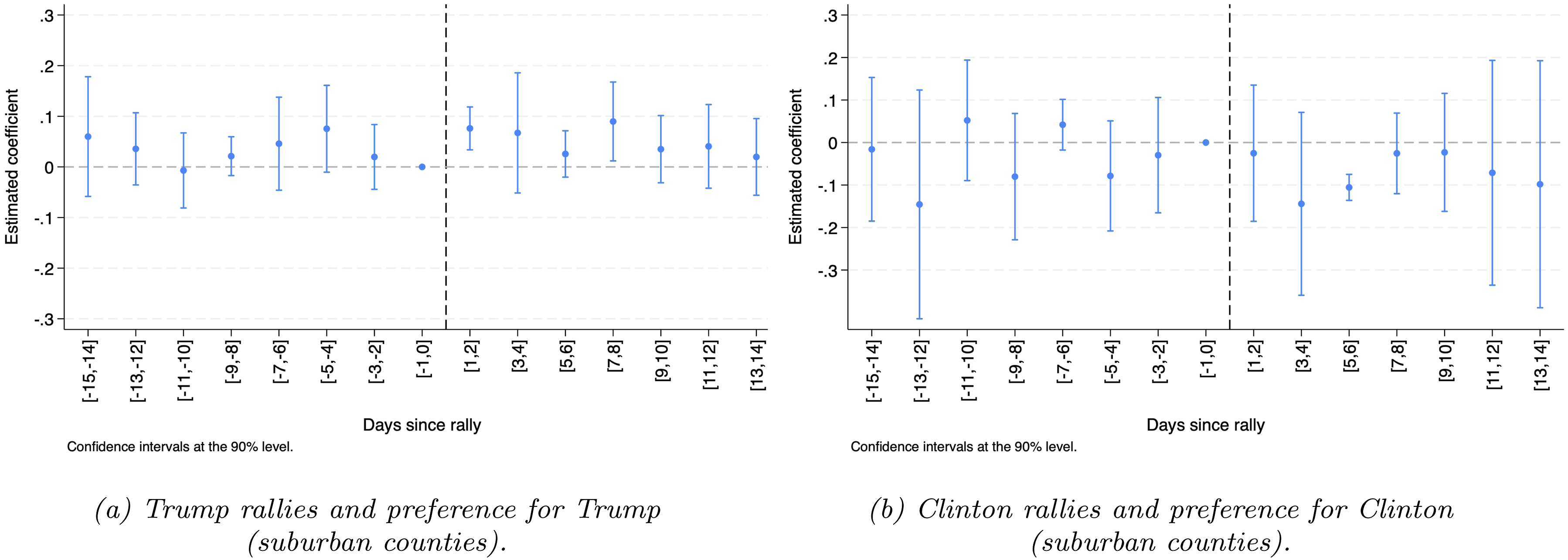
The effects of rallies in urban and suburban counties are presented in Figures 3 and 4, respectively. The patterns differ sharply across candidates. For Clinton rallies, the broad pattern is less suggestive of systematic geographic heterogeneity than for Trump rallies. While one post-rally bin in suburban counties is negative, the Clinton heterogeneity estimates are based on a substantially smaller suburban sample (1050 observations vs 3420 in urban counties) and do not yield robust differences in average effects across urban and suburban counties. For Trump rallies, pooling all counties masks substantial heterogeneity. In urban counties, support for Trump declines several days after a rally (the drop is not immediate and fades within roughly a week). In suburban counties, support increases right after the rally and remains elevated for about a week, with statistically significant effects in bins [1,2] and [7,8]. Estimates for the “Other” category are considerably noisier because of limited overlap between interviews and rallies, which resulted in a small number of observations being usable; they are shown in Figure C.1.OPEN IN VIEWER

Figure 3.

Effect of rallies on preferences over candidates in urban counties. This figure shows the coefficients retrieved from estimating equation (1) in the subsample of individuals living in urban counties visited by Trump and Clinton, respectively. Robust standard errors are clustered at the county-level.

OPEN IN VIEWER

Figure 4.

Effect of rallies on preferences over candidates in suburban counties. This figure shows the coefficients retrieved from estimating equation (1) in the subsample of individuals living in suburban counties visited by Trump and Clinton, respectively. Robust standard errors are clustered at the county-level.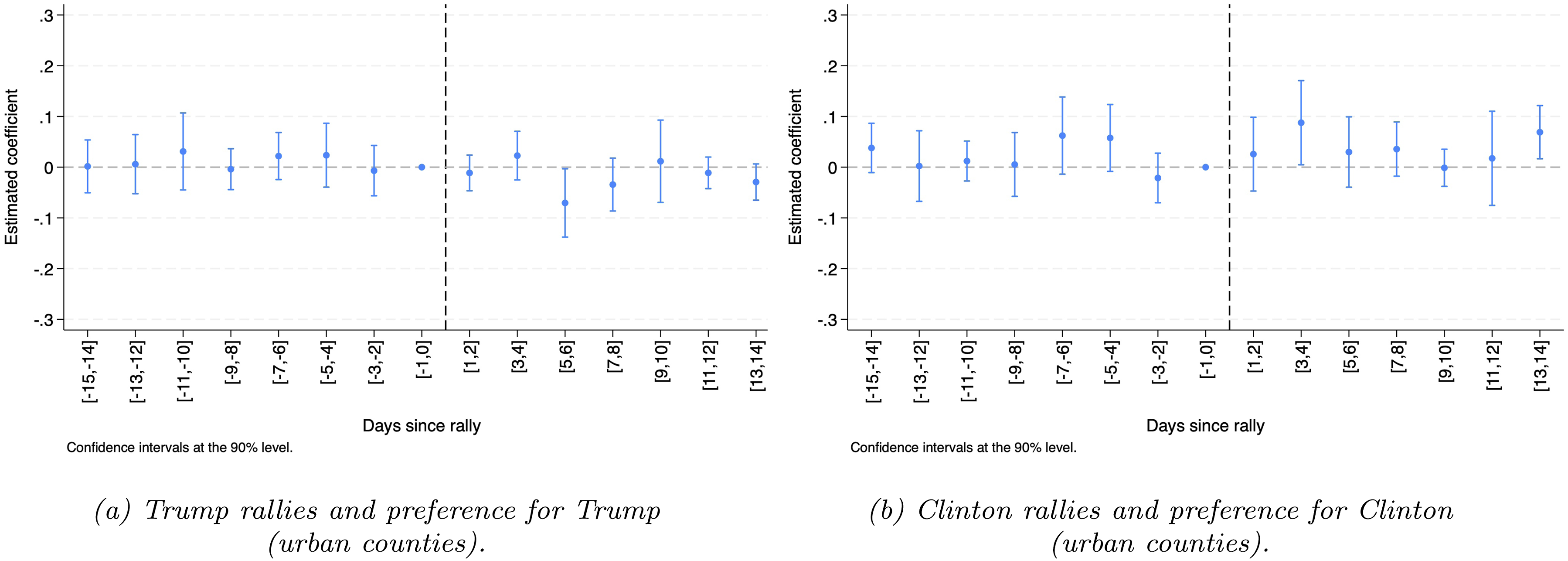

These dynamic effects are summarized in table C.2, which reports the average post-rally impact by county type using equation (2). The average effects mirror the event-time patterns: Trump rallies reduce stated support in urban counties but increase it in suburban counties, and the two effects are statistically different (an F-test rejects equality, p = 0.006). In contrast, there is no evidence that Clinton rallies have systematically different average effects across urban and suburban counties. Overall, the results point to a clear asymmetry: Trump rallies appear polarizing across geographies, while Clinton rallies look comparatively homogeneous.

Policy attitudes and ideology

CCES also measures support for a set of policies spanning gun control, immigration, abortion, the environment, and crime. I code each policy item so that 0 corresponds to the more right-leaning position and 1 to the more left-leaning position, and construct topic indices by averaging items within each topic. I then construct two overall ideology indexes following distinct approaches. The first one consists of averaging all issues included in the topic indices, so that higher values correspond to more left-leaning policy preferences. The second approach constructs an standardized index following (Anderson, 2008), which aggregates multiple policy outcomes into a single summary measure by standardizing each item, and weighting items using the inverse of their covariance matrix so that more redundant (highly correlated) items receive less weight. The resulting index is oriented so that higher values indicate more left-leaning preferences, and it improves statistical efficiency (relative to an unweighted average) when combining many related measures into one ideology score.

Table 2 reports average effects of rally exposure on policy indices. Overall, the estimates suggest limited policy persuasion. For Trump rallies, coefficients are small and generally not statistically different from zero in both urban and suburban counties, with one exception: in urban counties, the crime-policy index shifts modestly in a more Republican direction. For Clinton rallies, policy indices in urban counties show no clear systematic movement. In suburban counties, however, Clinton rallies are associated with a modest leftward shift in the summary ideology measures (both the simple-average index and the Anderson index), even though issue-specific estimates can be mixed across topics. Taken together, the policy results indicate that rallies mainly move candidate support, while issue positions respond more selectively.

OPEN IN VIEWER

Table 2.

The effect of Trump and Clinton rallies on policy preferences.

​	Guns	Immigration	Abortion	Environment	Crime	Ideology index
						Simple average	Anderson
	(1)	(2)	(3)	(4)	(5)	(6)	(7)
Panel A.1. Trump rallies: Urban counties
Trump rally	0.013	−0.024	−0.010	0.003	−0.024*	−0.007	−0.010
​	(0.016)	(0.023)	(0.023)	(0.012)	(0.012)	(0.011)	(0.008)
Mean (not exposed)	.665	.572	.584	.678	.543	.71	.733
R2	.28	.316	.324	.335	.242	.493	.265
N	3453	3453	3453	3453	3453	3453	3453
Panel A.2. Trump rallies: Suburban counties
Trump rally	0.012	0.029	0.005	−0.007	0.012	0.011	0.011
​	(0.015)	(0.033)	(0.020)	(0.026)	(0.034)	(0.012)	(0.011)
Mean (not exposed)	.679	.513	.629	.675	.535	.719	.75
R2	.298	.364	.416	.379	.303	.529	.29
N	1345	1345	1345	1345	1345	1345	1345
Panel B.1. Clinton rallies: Urban counties
Clinton rally	−0.016	−0.005	−0.001	−0.006	−0.008	−0.007	−0.002
​	(0.012)	(0.009)	(0.013)	(0.011)	(0.013)	(0.008)	(0.008)
Mean (not exposed)	.683	.574	.605	.677	.546	.724	.744
R2	.262	.313	.29	.302	.237	.483	.259
N	3420	3420	3420	3420	3420	3420	3420
Panel B.2. Clinton rallies: Suburban counties
Clinton rally	0.023**	−0.031*	0.042	0.032	−0.008	0.014*	0.025***
​	(0.008)	(0.015)	(0.034)	(0.025)	(0.007)	(0.006)	(0.006)
Mean (not exposed)	.69	.572	.615	.688	.543	.714	.741
R2	.382	.434	.487	.407	.375	.582	.342
N	1050	1050	1050	1050	1050	1050	1050

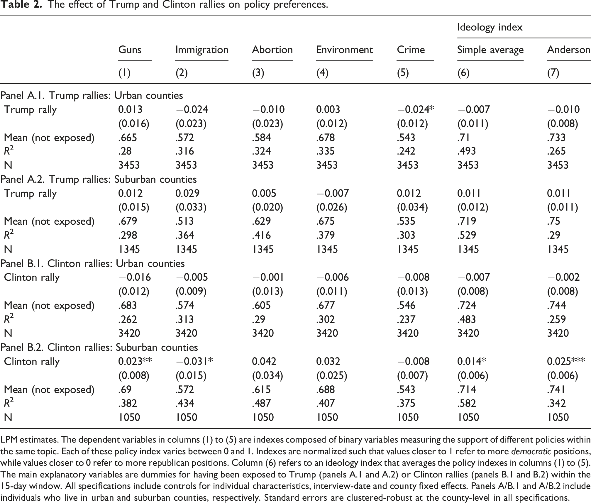
LPM estimates. The dependent variables in columns (1) to (5) are indexes composed of binary variables measuring the support of different policies within the same topic. Each of these policy index varies between 0 and 1. Indexes are normalized such that values closer to 1 refer to more democratic positions, while values closer to 0 refer to more republican positions. Column (6) refers to an ideology index that averages the policy indexes in columns (1) to (5). The main explanatory variables are dummies for having been exposed to Trump (panels A.1 and A.2) or Clinton rallies (panels B.1 and B.2) within the 15-day window. All specifications include controls for individual characteristics, interview-date and county fixed effects. Panels A/B.1 and A/B.2 include individuals who live in urban and suburban counties, respectively. Standard errors are clustered-robust at the county-level in all specifications.

Robustness and sensitivity

This section summarizes three robustness checks for the dynamic effects (full figures are reported in Appendix E).

Conclusion

This paper estimates the causal effects of campaign rallies on voters’ preferences over candidates and policies in the 2016 U.S. presidential election. The empirical strategy combines individual-level CCES survey data with detailed information on the timing and location of rallies, and exploits quasi-random exposure generated by the fine timing of interviews relative to rallies within the same county. Across specifications, the event-study profiles show little evidence of systematic pre-trends, supporting the interpretation that the observed post-rally dynamics largely reflect changes occurring after the event rather than differential trends already underway.

Three findings stand out. First, Clinton rallies increase stated support immediately after the event, fading within about 5 days; averaged over the event window, the preferred specification implies an increase of roughly 2 percentage points. Second, Trump rallies polarize geographically: support declines in urban counties several days after a rally (about 2 points on average) but rises in suburban counties (about 5-6 points) and remains elevated for roughly a week. Third, policy attitudes move less than candidate evaluations: Trump rallies show little consistent movement in issue positions, while Clinton rallies are associated with a modest leftward shift in suburban counties.

The transitory nature of the effects raises a broader question: if rallies do not durably shift stated preferences, why are they such a prominent campaign input? One implication is that rallies may matter primarily through channels not captured by persistent persuasion in county-level survey measures? Such as earned media, fundraising, mobilization, or strategic deterrence. The results are consistent with several (non-mutually exclusive) mechanisms. One interpretation is that, for most voters, exposure operates primarily through local information environments rather than direct attendance. First, rallies may be aimed less at persuading local attendees than at generating media coverage and amplifying campaign messages well beyond county borders. Under this view, rallies may increase the salience of candidates in local news cycles, generating short-lived shifts in attention that decay as coverage fades.

Consistent with this interpretation, descriptive evidence in Appendix F shows that Google search intensity and television mentions of the candidates rise around rally dates, peak on or near the event day, and then decline thereafter, mirroring the short-lived dynamics estimated in the survey data. This mechanism can also help rationalize the asymmetric patterns across candidates and geographies. Table F.1 shows that campaign geography differed across candidates in a nonlinear way: Clinton rallies were more concentrated in strongly Democratic counties, whereas Trump rallies were spread across a broader set of counties and were less concentrated at the most Democratic end of the distribution. This suggests that where candidates campaigned is part of the explanation for the asymmetry, but not the whole story. Mediated campaign messages may also generate both mobilization and counter-mobilization depending on the audience, leading to heterogeneous responses across locations, as suggested by Heersink et al. (2021).

Second, rallies may operate through durable margins even when persuasion is short-lived. For example, by stimulating fundraising, as emphasized by Snyder and Yousaf (2020) or Heersink et al. (2021). Third, rallies may reflect strategic interaction: even if the average persuasive return is limited, holding rallies can be an optimal defensive response to an opponent? Campaigning, shaping the pace and geography of campaign effort. A key limitation is that exposure is measured at the county-level and cannot capture attendance intensity, content, or cross-county spillovers. As a result, the effects documented here may understate persistence if measurement error attenuates estimates: the analysis does not observe who attends, what is said, or how rallies are covered and discussed, and higher-intensity exposure or systematically different rally content could plausibly generate longer-lasting effects. This interpretation also yields testable implications: if media is the main transmission channel, one would expect stronger effects in areas with higher local news penetration or greater coverage intensity, and effects that more closely track the timing of news cycles.

A second open question is how these short-run changes translate into electoral outcomes. Estimating the effect of rallies on actual vote shares is challenging with publicly available data. In particular, the post-election wave of the CCES lacks the within-county “before versus after” variation that underpins the design used here, and rally locations themselves may be endogenously chosen in response to electoral incentives. Future work could combine higher-frequency measures of beliefs and behavior closer to Election Day with richer data on rally content, attendance, and media spillovers, or develop a structural framework linking rallies to both persuasion and mobilization.

Supplemental material