New insights into elo algorithm for practitioners and statisticians

Abstract

This work reconciles two perspectives on the Elo ranking: the practitioner’s heuristic feedback rule, and the statistician’s online maximum likelihood estimation via stochastic gradient ascent. Both perspectives coincide exactly in the binary case if and only if the expected score is the logistic function. Estimation noise forces a principled decoupling between the model used for ranking and the model used for prediction: the effective scale and home-field advantage parameter must be adjusted to account for noise, with closed-form corrections and a data-driven identification procedure. For multilevel outcomes, an exact relationship exists when outcome scores are uniformly spaced, but approximations are preferred in general because they account for estimation noise, convergence, and better fit the data. Using synthetic and empirical (FIFA and FIVB) data, we show that the decoupled approach outperforms the conventional one that reuses the ranking model for prediction and serves as a convergence diagnostic. Convergence analysis indicates that FIFA men’s national teams had not converged for the vast majority of teams. The paper is written in a semi-tutorial style, with all key results accompanied by closed-form expressions and numerical examples.

Keywords

Bayesian analysis Bayesian statistics convergence football performance analysis predictive modeling

Introduction

The ranking in sports is used to decide which teams should be promoted/relegated between leagues or how to fix the competition format; it also provides a quick understanding of the relative strengths of the teams/players. Thus, it is of fundamental importance and has already attracted a consistent interest in sports, e.g., chess, football, e-sports, as well as in academic circles (Aldous, 2017; Glickman, 1995; Lasek and Gagolewski, 2018; Morel-Balbi and Kirkley, 2025; Tang et al., 2025).

Ranking algorithms/strategies were often devised by practitioners who, guided by their intuition and understanding of the competition, were able to propose practical solutions. Among the many algorithms, the Elo ranking (Elo, 1978) stands out due to its remarkable resilience and scope of application. Introduced by Arpad Elo in the context of chess ranking and today used by the governing bodies of Fédération Internationale des Échecs (FIDE) (FIDE, 2019) and Fédération Internationale de Football Association (FIFA) (FIFA, 2018), it has also been applied to theoretically analyze football (Csató, 2024; eloratings.net, 2020; Szczecinski and Roatis, 2022), basketball, American football (FiveThirtyEight, 2020), tennis (Kovalchik, 2020), and beyond.

This unquestionable success is easy to understand: the Elo algorithm is simple to implement, transparent in its logic, and adapts naturally to settings where competitors’ abilities evolve over time. However, we must agree with Aldous (2017) that Elo algorithm is indeed a case of “neglected topic in applied probability” whose theoretical understanding deserves more attention.

This is particularly true because the literature related to Elo ranking was dominated by the practitioner’s perspective, which sees the algorithm as a heuristic feedback rule: skills are updated in proportion to the gap between an observed match score and a pre-defined expected score (Cortez and Tossounian, 2026; Hvattum and Arntzen, 2010; Lasek et al., 2013). No probabilistic model is required, and the expected score function can be freely chosen, as was done in the original formulation by A. Elo (Elo, 1978). This also invites modifications, which mix probabilistic models and heuristics (Ingram, 2021; Kovalchik, 2020).

Although heuristics may be useful, they often lack the proper methodology to objectively evaluate the ranking, as this usually requires some kind of predictive capability, which in turn needs a probabilistic model linking the skills with the outcomes.

Recognizing this fundamental weakness, the statistician’s perspective,¹ always relies on the probabilistic model linking unobservable skills of competitors to matches outcomes, and the algorithm is interpreted as an online implementation of maximum likelihood (ML) estimation via stochastic gradient (SG) ascent (Király and Qian, 2017; Szczecinski and Djebbi, 2020; Tang et al., 2025), or through more sophisticated Bayesian update (Glickman, 1999; Ingram, 2021; Szczecinski and Tihon, 2023).

These two perspectives are not always distinguished carefully in the literature, and conflating them can lead to difficulties in interpreting and evaluating results. This is true for matches with two outcomes (win/loss) but even more so when multi-level outcomes must be used for ranking (e.g., win/draw/loss).

It should be noted that, in a large body of work on the ranking and modeling in sports, the statistician’s approach usually produces new algorithms, which may be similar to, but are not the same as the simple Elo algorithm. Needless to say, among the many ranking proposals e.g., (Angelini et al., 2022; Davidson and Beaver, 1977; Egidi and Ntzoufras, 2020; Ingram, 2021; Karlis and Ntzoufras, 2008; Kovalchik, 2020; Lasek and Gagolewski, 2021; Rao and Kupper, 1967; Szczecinski, 2022; Szczecinski and Djebbi, 2020), none succeeded in dethroning the Elo algorithm. Thus, our objective is not to develop yet another ranking algorithm to compete with Elo. Elo’s resilience across sports and decades speaks for itself. Rather, following the principle “if you cannot beat them, join them”, we aim to reconcile the two perspectives with two main goals: a) provide practitioners with principled tools to understand, interpret, and evaluate the Elo ranking, and b) give statisticians a less rigid framework by decoupling the ranking algorithm from the predictive model, so that Elo can be used efficiently without the need to replace it.

To bridge the two perspectives constructively, we focus on what is practically useful, build on previous work on the statistical foundations of Elo (Aldous, 2017; Gomes de Pinho Zanco et al., 2024; Király and Qian, 2017; Szczecinski, 2022; Szczecinski and Djebbi, 2020) and on the evaluation of Elo-based rankings (Szczecinski and Roatis, 2022), and make the following contributions:

We show a self-contained derivation of the equivalence between the practitioner’s Elo algorithm and ML estimation, for both binary and multilevel outcomes (Section “Practitioner meets statistician” and Section “Statistician’s perspective: Ordinal model and ranking algorithm”).

We quantify in simple terms the dependence of the estimation noise and the convergence speed on the adaptation step $K$ and the scale $s$ , generalizing the results of Gomes de Pinho Zanco et al. (2024).

We quantify the effect of estimation noise on predictive performance and show how the effective scale and the home-field advantage (HFA) parameter must be adjusted to account for it (Section “Interpretation of the skills”). The resulting correction clarifies and extends the results by Ingram (2021); Sonas (2011) by making explicit the role of the skills’ dispersion.

We postulate a model decoupling principle (Section “Interpretation of the skills” and Section “Decoupling prediction from ranking”) linking the Elo algorithm to the adjacent categories (AC) model that can be used for prediction.

Using synthetic, as well as empirical, FIFA and Fédération Internationale de Volleyball (FIVB) data, we show that simple closed-form formulas defining the AC model already capture most of the prediction gain.

The manuscript is structured in a semi-tutorial fashion to be accessible to practitioners. Section “Ranking from pairwise comparisons” treats the binary-outcome case, establishing the convergence properties, providing a probabilistic interpretation of the skills, and introducing the idea of scale adjustment due to estimation noise. Section “Beyond win/loss matches: Elo ranking for multilevel outcomes” extends the framework to multilevel outcomes, identifies the AC model underlying the Elo algorithm, and develops the model-decoupling approach with examples on synthetic, FIFA, and FIVB data. Numerical examples are integrated into text and, to simplify the flow, some mathematical derivations are relegated to Appendices.

Notation 1.
Throughout the paper, $(\cdot) $ denotes true* (but unknown) variables we use in simulations, e.g., $η $ . Thus, $θ _{m}$ denotes the true (unknown) skill of player $m$ , while $θ_{t, m}$ denotes its estimate at time $t$ , obtained from the Elo algorithm. The time index $t$ is omitted when the context makes it unambiguous. The hat notation $\hat{(\cdot)}$ is reserved for parameters estimated from data (e.g., $\hat{s}$ , $\hat{η}$ , $\hat{α}$ ). The notation $\tilde{s}$ / $\tilde{η}$ is used to denote parameters which must change under new modeling assumptions (e.g., scale $s$ under one model becomes scale $\tilde{s}$ under another). Vectors are denoted in bold (e.g., $θ_{t}$ , $x_{t}$ ).

Ranking from pairwise comparisons

We consider a scenario in which $M$ players/teams face each other in one-on-one matches indexed with $t = 1, \dots, T$ , where $T$ is the total number of matches. The results of the matches are denoted as $y_{t} \in Y = {0, \dots, L - 1}$ , where the outcomes are ordered by their desirability from the home player’s perspective, i.e., $y_{t} = L - 1$ is the most desirable outcome (e.g., a win) and $y_{t} = 0$ is the least desirable (e.g., a loss).

The objective of ranking is, after observing the matches $y_{t}$ , to characterize the performance of each player using a scalar parameter called “skill” (also known as “merit” or “strength” (Langville and Meyer, 2012; Newman, 2023)), denoted $θ_{t, m} \in R$ . By sorting the skills, we obtain a ranking: we interpret $θ_{t, m} > θ_{t, n}$ as player $m$ being “better” than player $n$ at time $t$ . The dependence on $t$ may be related to the time variability of skills (e.g., due to training or injuries).

The most popular assumption is that the difference in skills $z_{t} = θ_{t, i_{t}} - θ_{t, j_{t}}$ , where $i_{t}$ and $j_{t}$ identify the home and away players, suffices to model the match result.² Using the scheduling vector $x_{t} = e_{i_{t}} - e_{j_{t}}$ , where $e_{i}$ is the $i$ -th canonical basis vector (Szczecinski and Djebbi, 2020; Tang et al., 2025), and collecting skills in $θ_{t} = [θ_{t, 1}, \dots, θ_{t, M}]^{T}$ , we write
$z_{t} = x_{t}^{T} θ_{t} .$
(1)
Swapping home and away players maps $y_{t} \mapsto L - 1 - y_{t}$ and $z_{t} \mapsto - z_{t}$ .

Online ranking algorithms estimate $θ_{t}$ after each match recursively:
$θ_{t + 1} = ψ (θ_{t}, x_{t}, y_{t}),$
(2)
where $ψ (\cdot)$ denotes the update operator. We begin with binary outcomes ( $L = 2$ ), which simplifies the discussion; multilevel outcomes ( $L > 2$ ) are treated in Section “Beyond win/loss matches: Elo ranking for multilevel outcomes”.

Elo ranking in binary matches

Let us assume that we are dealing with binary matches i.e., $L = 2$ , where $y_{t} = 0$ denotes the loss of the home player $i_{t}$ and $y_{t} = 1$ indicates their win. Later, we will deal with the case of $L > 2$ , but the binary case simplifies the discussion and allows us to easily understand two perspectives on the well-known Elo ranking.

Practitioner’s perspective

The Elo ranking can be formulated from three elements:
A numerical score $ρ_{y} \in [0, 1]$ assigned to each outcome $y \in Y$ , increasing monotonically with $y$ . In the binary case,
$ρ_{y_{t}} = y_{t},$
(3)
i.e., $ρ_{0} = 0$ and $ρ_{1} = 1$ .

An expected score $G (z_{t}) \in [0, 1]$ , increasing in $z_{t}$ , satisfying the antisymmetry condition
$G (z_{t}) = 1 - G (- z_{t}),$
(4)
which ensures that the home and away perspectives are complementary: the expected scores for the home and away players sum up to $G (z_{t}) + G (- z_{t}) = 1$ .

A feedback update: skills are adjusted proportionally to the gap between observed and expected scores,
$θ_{t + 1} = θ_{t} + μ x_{t} [y_{t} - G (z_{t})],$
(5)
where $μ > 0$ is the step size, and (5) follows from applying the update symmetrically to home and away players via (4).

If $y_{t}$ is treated as a realization of a random variable $Y_{t}$ , then $G (z_{t}) = E_{Y_{t} | z_{t}} [ρ_{Y_{t}}]$ is a mathematical expectation, which for binary outcomes gives $G (z_{t}) = Pr {Y_{t} = 1 | z_{t}}$ . However, the practitioner may use $G (z_{t})$ informally without any probabilistic model — as is done in the FIDE (FIDE, 2019) and FIFA (FIFA, 2018) rankings, where $G (z_{t})$ is called “expected score” without reference to any underlying probabilistic model.

Statistician’s perspective

Using the practitioner’s perspective in Section “Practitioner’s perspective”, we interpret the expected score as the probability of the win, $G (z_{t}) = Pr {Y_{t} = 1 | z_{t}}$ . However, this is a side effect that was not required to derive the algorithm.

On the other hand, the statistician will always start by defining the model
$Pr {Y_{t} = y | θ } = P_{y} (z _{t}), y \in {0, 1},$
(6)
where $θ $ are unknown “true” skills we want to estimate and the probability depends on the skills’ difference $z _{t} = x_{t}^{T} θ $ .³

The practitioner’s assumptions are reproduced: $P_{1} (z _{t})$ must increase monotonically in $z _{t}$ (home win becomes more probable when $z _{t}$ grows), and home-away swap ( $z _{t} \leftarrow - z _{t}$ ) does not change the probability ( $y_{t} \leftarrow L - 1 - y_{t}$ , e.g., home win before swap becomes away win after swap)
$P_{y} (z) = P_{L - 1 - y} (- z),$
(7)
which in the binary case implies that
$P_{1} (z) = P_{0} (- z) = 1 - P_{1} (- z) .$
(8)

The skills, treated as unknown parameters of the model, can then be inferred using a preferred estimation method. For example, we may apply the ML principle
$\hat{θ} = \underset{θ}{argmax} \sum_{t \in T} ℓ_{y_{t}} (x_{t}^{T} θ),$
(9)
where $T$ is a batch of indices and
$ℓ_{y} (z_{t}) = \log P_{y} (z_{t})$
(10)
is the log-likelihood of $z_{t} = x_{t}^{T} θ$ for the observed match results $Y = y$ .

If instead of batch optimization (9) we opt for an on-line approach (2), we can use SG in the ML problem in (9). It boils down to the sequential update of the skills according to the following ML+SG algorithm:
$θ_{t + 1} = θ_{t} + μ \nabla_{θ_{t}} ℓ_{y_{t}} (z_{t})$
(11)
$= θ_{t} + μ x_{t} {\dot{ℓ}}_{y_{t}} (z_{t}),$
(12)
where
${\dot{ℓ}}_{y} (z_{t}) = \frac{d}{d z} ℓ_{y} (z) |_{z = z_{t}} = \frac{{\dot{P}}_{y} (z_{t})}{P_{y} (z_{t})},$
(13)
and $μ$ is the adaptation step. Since we focus on (12), the notation $\hat{θ}$ from (9) will not be reused.

Using (8), straightforward calculation gives
${\dot{ℓ}}_{y_{t}} (z_{t}) = [y_{t} - P_{1} (z_{t})] ϕ (z_{t}),$
(14)
$ϕ (z_{t}) = \frac{{\dot{P}}_{1} (z_{t})}{[1 - P_{1} (z_{t})] P_{1} (z_{t})},$
(15)
which used in (12) yields
$θ_{t + 1} = θ_{t} + μ x_{t} [y_{t} - P_{1} (z_{t})] ϕ (z_{t}) .$
(16)

Both practitioner and statistician know that to guarantee the convergences of the algorithm, we need a “sufficiently small” $μ$ which is often determined heuristically (with values $μ < 0.1$ usually working “well” but the exact conditions for convergence may be more involved (Gomes de Pinho Zanco et al., 2024)). On the other hand, only recognizing the algorithm as SG maximization, we know that we also need a concave form of $ℓ_{y} (z)$ – a condition that is satisfied for $P_{1} (z) = L (z)$ and $P_{1} (z) = Φ (z)$ .⁴

Practitioner meets statistician

If we decide to use $P_{1} (z_{t}) = G (z_{t})$ , (16) will be similar to (5). Both will be identical when $ϕ (z) \propto 1$ which, from (15), is satisfied if
${\dot{P}}_{1} (z) \propto [1 - P_{1} (z)] P_{1} (z) .$
(17)
This differential equation is uniquely solved⁵ by the logistic function
$P_{1} (z) = L (z / s)$
(18)
$L (z) = \frac{1}{1 + e^{- z}} .$
(19)

Thus, the only way to obtain the equivalence between the practitioner’s and statisticians’ rankings is by using $G (z) = L (z)$ . Indeed, this choice is often made in practice, and then the practitioner’s approach is endowed with a clear statistical interpretation of the ranking results: if we set $G (z) = L (z)$ , the Elo algorithm solves the ML estimation problem using the SG algorithm.

What happens when we set $G (z)$ arbitrarily? A natural example is $G (z) = Φ (z)$ , the Gaussian cumulative density function (CDF),⁶
$G (z) = Φ (z) = \frac{1}{\sqrt{2 π}} \int_{- \infty}^{z} \exp (- 0.5 x^{2}) d x .$
(20)
Setting $P_{1} (z) = Φ (z)$ gives $ϕ (z) ⧸ \propto 1$ , so the Elo algorithm implements ML+SG only approximately. However, since SG is itself an approximate solution, this distinction is rarely critical in practice.

The more important difference between the two perspectives is that the practitioner ignores estimation errors entirely, while the statistician treats $θ_{t}$ as noisy estimates of the true skills $θ $ . This has direct consequences for prediction, as we show in Section “Interpretation of the skills”. The statistician’s approach was made explicit much later than the practitioner’s, e.g., by Király and Qian (2017) and Lasek and Gagolewski (2021).

Re-scaling

The estimated skills in the vector $θ_{t}$ may be quite small,⁷ and it is customary to multiply them by the scale $s > 0$ , i.e., we make the replacements $θ_{t} \leftarrow s θ_{t}$ and $z_{t} \leftarrow s z_{t}$ , which integrated into the recursive estimation (5) produce
$θ_{t + 1} = θ_{t} + μ s x_{t} [y_{t} - G (z_{t} / s)]$
(21)
$= θ_{t} + K x_{t} [y_{t} - L (z_{t} / s)]$
(22)
where, in the conventional presentation of the Elo algorithm shown in (22), the scale is absorbed into step $K = μ s$ . However, leaving the scale in the notation (21) clarifies that by changing the scale from $s$ to $\tilde{s} = β s$ , to maintain the same algorithm behavior, we should also change the step from $K$ to $\tilde{K} = β K$ .⁸

Note that we decide to treat $G (z) = L (z)$ as a “canonical” form of the expected score in the Elo ranking. It also clarifies the role of scale, which is arbitrary, but useful when comparing different ranking algorithms. This is because the functions $G (z) \neq L (z)$ may be similar to $L (z)$ after appropriate scaling, i.e., $G (z / \tilde{s}) \approx L (z / s)$ .

For example, using, as the expected score, a generalized logistic function
$G (z) = L (z; a) = \frac{1}{1 + a^{- z}}$
(23)
with an arbitrary exponential basis, $a > 0$ , we can write
$L (z / \tilde{s}; a) = L (z / s),$
(24)
$\tilde{s} = s β_{e \to a},$
(25)
where we use a mnemonic notation
$β_{e \to a} = \log a,$
(26)
to indicate the scale adjustment required to replace the canonical logistic function $L (\cdot)$ with a generalized logistic function $L (\cdot; a)$ . In this particular case, after scaling (24), we obtain not only a similar but identical ranking algorithm regardless of the basis $a$ . Similarly, we can go from $L (\cdot; a)$ to $L (\cdot)$ using $β_{a \to e} = 1 / β_{e \to a}$ .

If we decide to use $G (z) = Φ (z)$ , the expected scores (and the ranking algorithms) can be made only approximately equivalent
$Φ (z / \tilde{s}) \approx L (z / s) .$
(27)
For example, the “equivalence” may be enforced by making the derivatives equal for $z = 0$ , i.e.,
$\frac{1}{\tilde{s}} \dot{Φ} (z / \tilde{s}) |_{z = 0} = \frac{1}{s} \dot{L} (z / s) |_{z = 0},$
(28)
where $\dot{Φ} (z) = \frac{d}{d z} Φ (z) = N (z) = \frac{1}{\sqrt{2 π}} \exp (- 0.5 z^{2})$ , and $\dot{L} (z) = L (z) L (- z)$ . This yields
$\tilde{s} = s β_{L \to Φ},$
(29)
$β_{L \to Φ} = \frac{4}{\sqrt{2 π}} \approx 1.6.$
(30)
Although somewhat arbitrary,⁹ this approximation principle has value of being simple.

In fact, the current versions of the Elo algorithm use the generalized logistic functions $L (z; 10)$ , however, the transformation between $Φ (z)$ and $L (z)$ is useful in approximate calculations we will see in Section “Interpretation of the skills”.

Home-field advantage and other effects

In practice, it is often observed that playing at home (that is, in the team stadium or the player’s country) provides an “advantage” to the player/team (Davidson and Beaver, 1977). Depending on the sport, this is known as the home-field/court/ice/ground advantage.

The HFA effect is modeled by increasing the difference $z_{t}$
$θ_{t + 1} = θ_{t} + K x_{t} [y_{t} - G (z_{t} / s + η h_{t})]$
(31)
$= θ_{t} + K x_{t} [y_{t} - G ((θ_{t, i_{t}} - θ_{t, j_{t}} + η s h_{t}) / s)]$
(32)
where $η$ is the scale-independent factor HFA and $h_{t} = 1$ indicates that the match is played at the player’s home venue (country/arena / stadium) and $h_{t} = 0$ indicates the neutral venue (e.g., during competitions hosted by a country different from the home and away players). To simplify the notation, we assume that $h_{t} = 1$ .

The formulation in (31) corresponds to increasing the skills of the home player by $s η$ , which, alternatively, may be seen as a value by which the skills of the away player must be increased to neutralize the effect of HFA. The meaning of HFA can be naturally extended to any identifiable element that favors the home player. For example, in chess, the player starting with white pieces has, on average, better chances of winning.

Similarly, in the statistician’s approach, we use
$Pr {Y_{t} = 1 | z} = P_{1} (z_{t} / s + η),$
(33)
and can also directly modify the algorithm (12)
$θ_{t + 1} = θ_{t} + μ s x_{t} {\dot{ℓ}}_{y_{t}} (z_{t} / s + η) .$
(34)

If we want to change the expected score, e.g., from $G (z / s)$ to the canonical logistic function $L (z / \tilde{s})$ this is done as follows:
$G (z_{t} / s + η) = G ((z_{t} + η s) / s)$
(35)
$\approx L ((z_{t} + η s) / \tilde{s}) = L ((z_{t} + \tilde{η} \tilde{s}) / \tilde{s})$
(36)
$= L (z_{t} / \tilde{s} + \tilde{η}),$
(37)
$\tilde{s} = s β,$
(38)
$\tilde{η} = η / β,$
(39)
where $β$ is the scale adjustment factor, e.g., $β = 1 / β_{e \to a}$ or $β = 1 / β_{L \to Φ}$ (depending on whether we go to $L (z / \tilde{s})$ from $G (z / s) = L (z / s; a)$ or $G (z / s) = Φ (z / s)$ ) and $\tilde{η}$ is the new HFA term to be used in the canonical logistic score, and we preserve the product $η s = \tilde{η} \tilde{s}$ .

For example, $η s = 100$ and $s = 400$ in eloratings.net (2020) (i.e., $η = 0.25$ ) which uses $G (z) = L (z; 10)$ so, by moving the algorithm to the canonical form $L (z)$ , we should use $β = 1 / β_{e \to 10} = 0.43$ and $\tilde{s} = s β \approx 174$ with $\tilde{η} = 0.25 / β \approx 0.58$ or $\tilde{η} \tilde{s} = 100$ .

Thus, if we want to rescale the skills in the same algorithm (the same expected score), the term $η$ should be kept separated from the scale, i.e., the notation $G (z / s + η)$ is useful, but if we change the function defining the expected score, the product $η s$ is preserved across the functions.

Other effects

Similarly to the HFA, other variables may be introduced into the ranking and prediction framework, e.g., type of venue, travel time before the game, or absence of key players, etc. This must be done carefully, understanding whether the variable belongs to the probabilistic model* or to the optimization strategy which can be decided by answering the following question: can the variable be used to predict the outcome of a future match? If yes (e.g., HFA), it belongs to the model. If no, it is part of the optimization strategy only.

A notable example of the latter is the variable adaptation step $K \equiv K (κ_{t})$ , used e.g., by FIFA and FIVB, which scales the update according to the declared “match importance” $κ_{t}$ . Since the latter does not help predict the outcome of a future game, it is a heuristic optimization strategy (e.g., justified by acceleration of the SG convergence after high-stakes matches) and not part of the probabilistic model.

Convergence

The detailed description of the dynamics defined through (21) is rather complex, see Cortez and Tossounian (2026), Jabin and Junca (2015), but is analyzed by Gomes de Pinho Zanco et al. (2024) in terms of the average variance of the skill estimate after convergence
$\bar{v} = lim_{t \to \infty} {\bar{v}}_{t},$
(40)
${\bar{v}}_{t} = \frac{1}{M} \sum_{m = 1}^{M} E [(θ_{t, m} - E [θ_{t, m}])^{2}],$
(41)
where the approximation proposed by Gomes de Pinho Zanco et al. (2024: Eq.(50)) is simplified to
$\bar{v} \approx s^{2} μ / 2 = s K / 2,$
(42)
where we assumed $K / s ≪ 1$ .

If the outcomes $y_{t}$ are generated using the model (33) with scale $s $ , we can assume that $E [θ_{\infty, m}] = θ_{m} s / s $ , that is, the ground truth must be rescaled; this will be taken into account and, unless stated otherwise, we use $θ_{m} \equiv θ_{m} * s / s $ . The variance $\bar{v}$ has a theoretical meaning because it can be measured only with multiple realizations of $θ_{t, m}$ which exist only in simulations; in practice, it can be calculated by temporal averaging as
${\bar{v}}_{t} \approx \frac{1}{W} \sum_{τ = - W + 1}^{t} | θ_{τ, m} - {\bar{θ}}_{t, m} |^{2},$
(43)
${\bar{θ}}_{t, m} \approx \frac{1}{W} \sum_{τ = - W + 1}^{t} θ_{τ, m},$
(44)
where $W$ is the length of the averaging window.

Moreover, Gomes de Pinho Zanco et al. (2024: Sec. 3.3) tells us that the skills converge in expectation as
$E [θ_{t^{'}, m}] \approx e^{- t^{'} / τ} (θ_{0, m} - E [θ_{\infty, m}]) + E [θ_{\infty, m}],$
(45)
where $t^{'} = 0, 1, \dots$ are the indices of the matches in which player $m$ is participating, and the convergence time constant given by¹⁰
$τ = \frac{4 s}{K} \sqrt{1 + v_{θ} / s^{2}},$
(46)
with $v_{θ}$ being the empirical variance of true skills in $θ $ . Thus $τ = 4 s / K$ is a lower bound on the time constant, achieved in the limit $v_{θ} \to 0$ of a perfectly balanced competition. For larger $v_{θ}$ , the time constant grows and convergence slows. Intuitively, when the skill spread is large, most matchups are highly unbalanced: the outcome is nearly certain, so $G (z_{t} / s)$ is close to $0$ or $1$ , the residual $ρ_{y} - G (z_{t} / s)$ is small, and each match carries little information about the true skill difference.

In practice, it is common to use variable adaptation step $K_{t}$ (defined, e.g., in FIFA ranking, according to the importance of the match (FIFA, 2018), or, in FIVB ranking, according to the number of matches played). In such a case, the variance and the time constant are obtained using the average adaptation step
${\bar{τ}}_{m} = \frac{4 s}{{\bar{K}}_{m}},$
(47)
$\bar{v} = \frac{1}{M} \sum_{m = 1}^{M} \frac{s {\bar{K}}_{m}}{2},$
(48)
${\bar{K}}_{m} = \frac{1}{N_{m}} \sum_{t_{t} = m \lor j_{t} = m} K_{t},$
(49)
where $N_{m}$ is the number of matches played by player $m$ .

After $2 {\bar{τ}}_{m} - 3 {\bar{τ}}_{m}$ matches, the convergence in expectation can be declared for player $m$ Gomes de Pinho Zanco et al. (2024: Sec. 4.2). We thus immediately note that the number of matches played alone does not explain the convergence as it also depends on the adaptation steps $K_{t}$ in those matches. More on that in Example 5.

Generally, for a given scale $s$ , increasing $K$ (or $K_{t}$ ) increases the convergence speed (the convergence time is inversely proportional to $K$ ) at the expense of higher estimation errors after convergence (the variance grows linearly with $K$ ). We illustrate this in Example 1.
Example 1 (Illustration of convergence).

We show in Figure 1 an example obtained from simulations, where $M = 30$ players with skills $θ *_{m}$ (generated using the Gaussian distribution with variance $v_{θ} = 0.5$ ) compete in a round-robin fashion with random matchups: at time $t$ each player is matched with a randomly chosen opponent (this is a random $x_{t}$ ) and the outcome of the match $y_{t}$ is generated with $P_{1} (z) = L (x_{t}^{T} θ * + η *)$ , where $η * = 0.35$ ; thus, the scale is $s * = 1$ .

Figure 1.

Trajectories of the estimated skills obtained using the Elo algorithm with random step 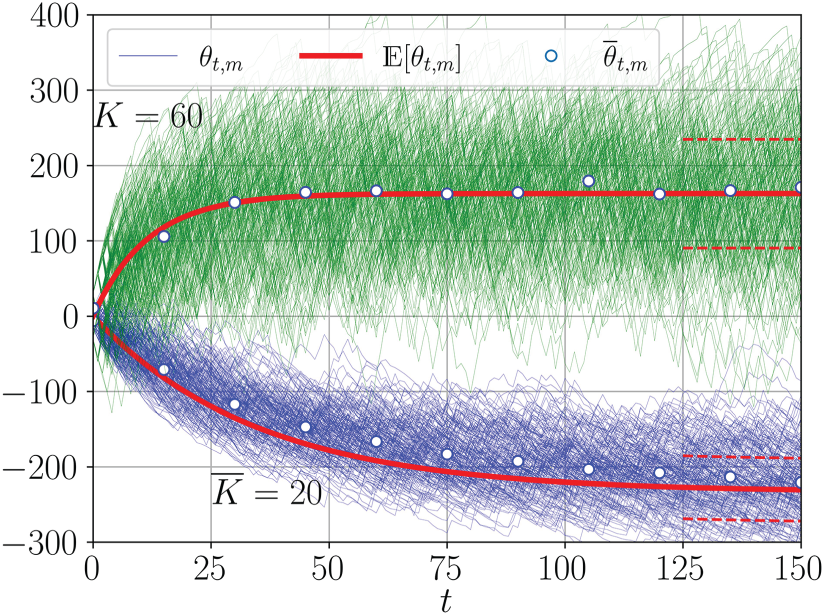$K_{t} \in {10, 20, 30}$ (lower, blue) or with fixed $K = 60$ (upper, green). Done for a given $θ *$ , each curve corresponds to a different realization of $y_{t}$ and $x_{t}$ . Markers indicate the empirical average (across realizations) and the dashed red lines indicate the 68% credible interval at convergence ( $E [θ_{\infty, m}] \pm \sqrt{\bar{v}}$ ).

The Elo algorithm uses the canonical expected score $L (z / s + η)$ with $η = η *$ and the scale $s = 174$ .¹¹ We consider two adaptation steps a) fixed $K = 60$ , and b) random $K_{t}$ selected with uniform probability from the set ${10, 20, 30}$ , thus we have $\bar{K} = 20$ . For two selected players, the trajectories of their skills $θ_{t, m}$ are shown with thin lines (blue when $\bar{K} = 20$ and green when $K = 60$ ) for $J = 200$ different realizations of $x_{t}$ and $y_{t}$ . The thick red curve indicates the analytical mean $E [θ_{t, m}]$ , the blue marker indicates the empirical mean, and the dashed red lines – the mean plus/minus the standard deviation $E [θ_{t, m}] \pm \sqrt{\bar{v}}$ (which is a rudimentary credible interval for $θ_{t, m}$ ). The analytical formulas give a reasonable prediction for a constant step $K$ and random $K_{t}$ .

Using random $K_{t}$ , the average time constant (46) is equal to $\bar{τ} = 4 \tilde{s} / \bar{K} \approx 4 \cdot 174 / 20 \approx 35$ , which means that after $2 τ - 3 τ \approx 70 - 104$ matches, the convergence in expectation may be declared. For $K = 60$ , $2 τ - 3 τ \approx 35 - 50$ . The differences in time constants can be seen in the behavior of the curves shown in Figure 1.

The variances (42) $\bar{v} = \bar{K} \tilde{s} / 2 \approx 1740$ (for $\bar{K} = 20$ ) and $\bar{v} = 5220$ (for $K = 60$ ) were reasonably close to the corresponding values $\approx 1762$ and $\approx 5807$ obtained empirically.

Remark on approximations. The analysis above assumes (i) stationary true skills $θ *$ and (ii) random scheduling. As for (i), slow skill evolution relative to the convergence dynamics justifies a local stationarity approximation. As for (ii), players competing rarely simply accumulate $τ$ matches more slowly in calendar time, and their opponents’ estimation errors act as additional noise, increasing effective variance above $\bar{v} \approx s K / 2$ . The qualitative conclusions nevertheless remain valid: $τ \propto 1 / K$ , variance $\propto K$ , and infrequent competitors converge more slowly.

At the core of the approximation is the assumption that $x_{t}$ is independent of $y_{t}$ and $θ_{t}$ . Rating-based scheduling reduces the effective skill dispersion seen by the estimator, amplifying $β_{err}$ in (60). A rigorous treatment of this dependence is beyond the scope of this work; the data-driven identification (62) should capture this effect automatically without requiring assumptions on the matchmaking mechanism.

Interpretation of the skills

Who is better?

If we need the ranking algorithm to find which team/player is stronger/better, it should be done comparing the estimated skills.

For the practitioner, there is no problem here: $θ_{t, m} > θ_{t, n}$ means that the team $m$ is better than the team $n$ . The statistician, on the other hand, is aware that the skills $θ_{t, m}$ are corrupted by the estimation errors $ξ_{t, m}$ , i.e., $θ_{t, m} = θ *_{t, m} + ξ_{t, m}$ , and thus

z_{t} = z *_{t} + ζ_{t},

(50)

where

z *_{t} = θ *_{t, i_{t}} - θ *_{t, j_{t}}

is the difference between the true skills and

ζ_{t} = ξ_{t, i_{t}} - ξ_{t, j_{t}}

is the difference between the estimation errors.

As a consequence of (50), the question “is $m$ better/worse than $n$ ?” (i.e., is $z *_{t} ≷ 0$ ?) can only have a probabilistic answer. The probability of the player $m$ being worse ( $z *_{t} < 0$ ) when we observe a particular value of the difference $z_{t}$ , is

Pr {z *_{t} < 0 | z_{t}} = Pr {ζ_{t} > z_{t} ∣ z_{t}} .

(51)

Assuming

ζ_{t} \sim N (0, 2 \bar{v})

, (51) becomes

Pr {z *_{t} < 0 | z_{t}} = Φ (- \frac{z_{t}}{\sqrt{2 \bar{v}}}) = Φ (- \frac{z_{t}}{\sqrt{K s}}) .

(52)

For example, with the observed positive skill difference $z_{t} = \sqrt{K s}$ , $Pr {z *_{t} < 0 | z_{t}} = Φ (- 1) \approx 0.16$ , i.e., there is still a $16 %$ chance of getting a wrong order between players.

The assumption of $ζ_{t}$ being Gaussian is only a conceptual device whose usefulness can be assessed using the simulation results of Fig 1 that produce the relationship shown in Figure 2.

Figure 2.

Probability of the Comparison between the empirical results and the formula (52) using the data from Figure 1.

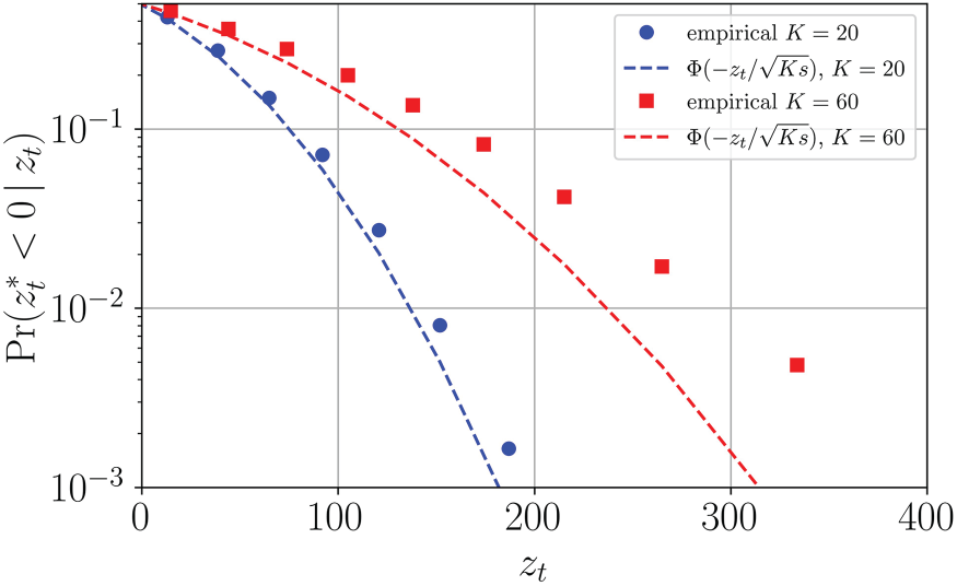
We see that the Gaussian model is optimistic but it provides a useful insight into the problem: for the chances of incorrectly ordering the players to be lower than 10 $-$ 15%, we may require the difference between the skills to be at least larger than $\sqrt{K s}$ .

Note that this condition is not easily satisfied. For example, the FIDE ranking (where the smallest step is $K = 16$ and the canonical scale is the same as in Example 1) published in March 2026 shows that the differences between the skills in top $-$ 20 consecutive positions are smaller than $20$ . Using (52) we get $Pr {z *_{t} < 0 | z_{t}} = Φ (- 20 / \sqrt{16 \cdot 174}) \approx 0.35$ . Thus, there are at least $35 %$ chances of placing any two consecutive top $-$ 20 players in a wrong order; this also means that declaring confidently who is the best is not really possible!

Prediction/performance evaluation

The prediction of the outcome of the match from the previous observations is reduced to the prediction from the estimated skill, that is, we want to find $Pr {Y_{τ} = y | θ_{t}}$ for any $τ \geq t$ .

This may be useful to analyze the structure of the tournament, e.g., (Csató, 2023; Lapré and Amato, 2025), to evaluate the betting odds (Egidi et al., 2018), to predict the outcomes of a competition (Brandes et al., 2025), or to compare the quality of the ranking models/algorithms (Gelman et al., 2014: Sec. 2).

In these cases, the relevant metric is the logarithmic probability of future matches $ℓ_{y_{τ}} (z_{t}) = \log Pr {Y_{τ} = y_{τ} | θ_{t}}$ that can be averaged across the testing set (of matches with the indices in $T^{test}$ ) to produce the mean logarithmic score.

L S = - \frac{1}{| T^{test} |} \sum_{τ \in T^{test}} ℓ_{y_{τ}} (x_{τ}^{T} θ_{t} / s + η),

(53)

where negation is optional but yields a positive log-scores with lower value meaning a “better” prediction. The main formal requirement is that

θ_{t}

not be calculated using

y_{τ}

. In the Elo ranking

y_{t}

affects

θ_{t + 1}

, so we can use the entire data set for testing, i.e.,

T^{test} = T

The task at hand seems simple for the practitioner: it is enough to use the model which appeared in Section “Practitioner’s perspective” and calculate

ℓ_{y_{t}} (z_{t}) = \log L (z_{t} / s + η) .

(54)

For the statistician, on the other hand, the model (18) connects the true skills $θ *_{m}$ to the outcomes $y_{t}$ , so the relationship to the noisy skills $θ_{t, m}$ (and thus also to $z_{t}$ ) can be found by marginalization over $z *_{t}$

\bar{L} (z *_{t} / s + η) = \int L (z *_{t} / s + η) f (z *_{t} | z_{t}) d z *_{t}

(55)

where

f (z *_{t} | z_{t}) \propto f (z_{t} | z *_{t}) f (z *_{t}) / f (z_{t}),

(56)

that is, we model the true

z *_{t} = θ *_{t, i_{t}} - θ *_{t, j_{t}}

as random variables, which makes sense because

i_{t}

and

j_{t}

are randomly selected and it is common to assume that the skills

θ *_{t}

are realizations of the random variables drawn from a Gaussian distribution with variance

v_{θ}

. Then

z *_{t}

can be thought of as a realization of a Gaussian variable with variance

2 v_{θ}

, i.e.,

f (z *_{t}) = N (z *_{t}; 0, 2 v_{θ})

To calculate (55) in closed form, we assume again that $ξ_{t, m}$ are zero-mean Gaussian variables with variance $\bar{v}$ , i.e., $f (z | z *) = N (z; z *, 2 \bar{v})$ and then, as shown in Appendix A, we have

\bar{L} (z *_{t} / s + η) \approx L (z_{t} / \hat{s} + \hat{η}) = L ((z_{t} + η s a) / \hat{s})

(57)

where

\hat{s} = s β_{err},

(58)

\hat{η} = \frac{η a}{β_{err}},

(59)

are the effective scale and HFA,

β_{err} = a \sqrt{1 + \frac{2 \bar{v}}{a (s β_{L \to Φ})^{2}}},

(60)

is the scale adjustment factor due to the estimation errors,

a = (1 + \bar{v} / v_{θ})

is defined in (119), and

β_{L \to Φ}

is the scale adjustment (30) used for model equivalence in Appendix A.

The average log-score (53) is then calculated as

L S = - \frac{1}{| T |} \sum_{t \in T} ℓ_{y_{t}} (z_{t} / \hat{s} + \hat{η}) .

(61)

Only if we neglect the estimation errors, i.e., when $\bar{v} \approx 0$ , we have $β_{err} \approx 1$ . This is what happens in (54) because, in the practitioner’s perspective, the estimation errors are not present.

Pseudo model-identification

Since the analytical formulas rely on assumptions and unknown parameters: $v_{θ}$ , Gaussian errors $ζ_{t}$ , etc, we may prefer to find the parameters $\hat{s}$ and $\hat{η}$ from the data directly through the following optimization:

\hat{γ}, \hat{η} = \underset{s, η}{argmax} \sum_{t} ℓ_{y_{t}} (γ z_{t} / s + η),

(62)

\hat{β} = 1 / \hat{γ};

(63)

for given

z_{t}

, the function under optimization is concave in

η

and in

γ

(but not concave in

β = 1 / γ

While this is a formulation typical in the ML model identification problems, we are not identifying the model per se but rather the joint effect of (i) the estimation noise in $z_{t} = x_{t}^{T} θ_{t}$ , (ii) the bias introduced by the limited variance $v_{θ}$ , and of (iii) the mismatch between the data and the models used in the estimation/ranking and the performance evaluation (in this synthetic example, there is no mismatch: all models are logistic).

After convergence, we always have $β_{err} > 1$ , thus the effective scale $\hat{s}$ increases with the noise in the skills’ estimates, $\bar{v}$ , but also with the ratio $\bar{v} / v_{θ}$ . Recognizing the latter, differs from the literature that often assumes only $\bar{v}$ affects the prediction (e.g., Ingram (2021: App. E)), which is true if $v_{θ}$ is sufficiently large, i.e., if the dispersion of the skills $θ_{t} *$ is much larger than the variance of the estimation errors; then $f (z *_{t} | z_{t}) = f (z_{t} | z *_{t})$ .

Example 2 (Fit to the estimated data).

Let us reuse Example 1 to find the scales through a fit to the estimated data where $T = 2000$ last matches after the convergence were used.

The results are shown in Table 1, where we see that (a) with growing estimation errors the scale

\hat{s}

increases and the effective HFA

\hat{η}

decreases, (b) the theoretical formulation in (58) explains quite well the results obtained through the actual fit to the data (62), and that (c) the scale fitting does not provide any meaningful gain for

K = 20

, but an improvement can be seen for

K = 60

, i.e., in the context of larger estimation errors.

Table 1.
Log-score (61) computed using the practitioner approach (assuming no estimation error), the theoretical approach (58) and (59), and the data-fitting approach based on (62). Here $s = 174$ , $η * = 0.35$ , $M = 30$ , $T = 1000$ . Values in parentheses denote (mean, std.) obtained from $J = 200$ realizations.

	$K = 20$			$K = 60$
Method	$\hat{β}$	$\hat{η}$	$L S$	$\hat{β}$	$\hat{η}$	$L S$
Assume no error	$1$	$η *$	$(0.59, 0.01)$	$1$	$η *$	$(0.62, 0.01)$
Theoretical	$1.10$	$0.34$	$(0.59, 0.01)$	$1.40$	$0.33$	$(0.60, 0.01)$
Data-fit	$(1.13, 0.04)$	$(0.34, 0.04)$	$(0.59, 0.01)$	$(1.45, 0.05)$	$(0.33, 0.04)$	$(0.60, 0.01)$

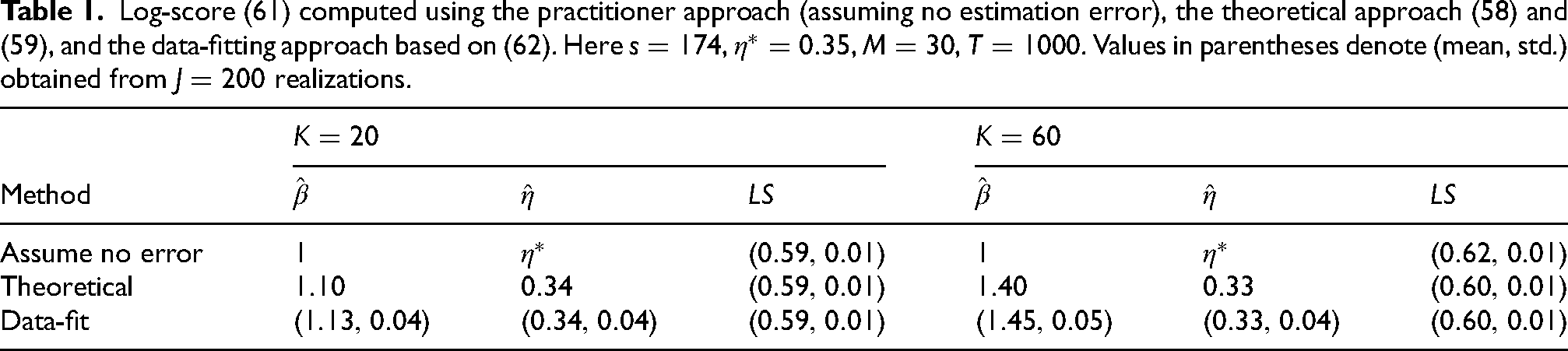
The formula (60) explains quite well why the actual fit to the data via (62) produce $\hat{s} > s$ and $\hat{η} < η *$ . On the other hand we know that the discrepancies may be produced by the estimation error and/or the distribution of the skills as defined via $v_{θ}$ and any other mismatch between the model and the data. What finally counts, is how to estimate the performance and, using $\hat{s}$ and $\hat{η}$ provides a simple answer. In that sense, (62) seems to be a more practical approach which does not need any assumptions required to derive (42).

Another reason to use (62) is that (60) works after convergence. On the other hand, before convergence is attained, the skills may be “compressed” when initialization $θ_{0, m}$ is smaller than $θ_{0, m} *$ . In this case the skills differences may be too small, i.e., $| z_{t} | < | z *_{t} |$ . Then, the theoretical formulas fail, but the empirical fit will unveil the lack of convergence by decreasing the scale $\hat{s}$ , that is, producing $\hat{β} < 1$ .

As shown in Table 1, in some cases, the scale fitting may appear superfluous. However, it is not a costly operation and is helpful when dealing with large estimation errors. More importantly, it introduces a key idea that the model used for ranking need not be the same as the one used for prediction. This conceptual model “decoupling” will be necessary when the model underlying the Elo algorithm is not explicitly specified; more on that in Section “Decoupling prediction from ranking”.

Note that instead of pseudo-fitting the model, we may also find the expected score $L (z / \hat{s} + \hat{η})$ from the data: this was done by Sonas (2011) via histogram of the score $ρ_{y_{t}}$ , which found the scale $\hat{s} \approx 1.25 s$ . However, Sonas (2011) did not explain that phenomenon, most likely because, adopting the practitioner’s perspective, the estimation errors were simply not taken into account.

Take-away insights:

The fact that we can have the “nominal” expected score $L (z / s + η)$ and the empirical expected score $L (z / \hat{s} + \hat{η})$ may lead to confusion: which one “is true”? In fact, both are correct but address different questions: the nominal one (which applies to the noise-free difference $z *_{t}$ ) drives the algorithm, while the empirical one applies to the estimated $z_{t} = z *_{t} + ζ_{t}$ and is useful in prediction.¹² After convergence, $\hat{s} = \hat{β} s$ where $\hat{β} > 1$ compensates for noise-induced uncertainty; before convergence, $\hat{β} < 1$ signals that skill differences are compressed toward initialization.

The Gaussian models are used here as purely descriptive tools that help build intuition before confronting it with empirical reality. In practice, only the latter matters, which is why the data-driven fit (62) is the preferred approach: it requires no knowledge of hypothetical Gaussian distributions. Figure 2 and Table 1 confirm that the insights provided are accurate enough to be practically useful.

Beyond win/loss matches: Elo ranking for multilevel outcomes

The binary-outcome Elo algorithm has a clean probabilistic interpretation only because the logistic function is the unique expected score that connects the practitioner’s and statistician’s perspectives (Section “Practitioner meets statistician”).

For multilevel outcomes [e.g., draws in football and chess, set margins in volleyball ( $L = 6$ ), overtime/shootout outcomes in ice hockey ( $L = 4$ )], no such connection exists and designers have typically fallen back on heuristics: choosing scores $ρ_{y}$ intuitively (for the draw $ρ_{1} = 0.5$ ) without specifying a probabilistic model.

The FIVB ranking illustrates the tension between competing practitioner’s and statistician’s objectives. It uses $L = 6$ outcomes and a cumulative link (CL) model (FIVB, 2024; Tenni et al., 2025), reflecting the statistician’s need for proper probabilistic foundations; but, as explained by Tenni et al. (2025), the update itself mimics the Elo algorithm without probabilistic justification, reflecting not only the practitioner’s attachment to the simple feedback rule but also the imprint left by decades of dominance of the Elo ranking. The FIVB algorithm is thus sitting on the fence without committing to either side: the statistical model is there formally, but the Elo heuristic is there in practice.

Our perspective on the Elo algorithm releases this tension by providing a principled connection between the algorithm and the model. For the practitioner, it identifies the unique probabilistic model that is implicitly optimized by the Elo algorithm with uniform scores (Proposition 1), while, for the statistician, the AC model is shown to play the same unifying role in the multilevel case that the logistic model plays in the binary case (Proposition 2). This justifies the model decoupling in Section “Decoupling prediction from ranking”.

Practitioner’s perspective: Simplicity!

The principles underlying the practitioner’s version of the Elo algorithm are so simple that the algorithm can also be used when matches have multilevel outcomes, i.e., when $L > 2$ . This is done “naturally” so the algorithm works as before, i.e., (31)

θ_{t + 1} = θ_{t} + K x_{t} [ρ_{y_{t}} - L (z_{t} / s + η h_{t})],

(64)

where, to focus the analysis, we use the logistic function (19) as the expected score, i.e.,

G (z) = L (z)

To apply the algorithm, we only need to assign numerical scores to the match’s results, i.e., $ρ_{y} \in [0, 1], y = 0, \dots, L - 1$ where we use $ρ_{0} = 0$ is the score of the least desirable outcome and $ρ_{L - 1} = 1$ – of the most desirable one. The scores $ρ_{y}$ will be monotonic in $y$ , as the practitioner will assign a higher score to a more desirable outcome $y$ ; we store them in a vector $ρ = [ρ_{0}, \dots, ρ_{L - 1}]$ .

In fact, this practitioner’s perspective has been the basis for the Elo algorithm devised to rate chess players (Elo, 1978), where matches can end in a draw (pat), for which the score was defined as $ρ_{1} = 0.5$ but where no probabilistic model was specified for three possible outcomes of the match.

Regarding the model, we recall that, at the end of Section “Practitioner’s perspective”, for $L = 2$ , the “expected score” was defined using the mathematical expectation interpretation, i.e.,

G (z) = \sum_{y = 0}^{L - 1} P_{y} (z) ρ_{y} .

(65)

For $L = 2$ , (65) implies a unique probabilistic model, $P_{1} (z) = G (z)$ and $P_{0} (z) = 1 - G (z)$ . However, for $L > 2$ , there is no such relationship and this leads to the following question: What probabilistic model, if any, underlies the algorithm (64)?

To answer it, we will continue treating the Elo ranking (64) as the ML+SG optimization (34) based on the derivative of unknown log-likelihood ${\tilde{ℓ}}_{y} (z)$ , that is,

θ_{t + 1} = θ_{t} + μ s x_{t} {\dot{\tilde{ℓ}}}_{y} (z / s + η),

(66)

where the derivative is given in (64)

{\dot{\tilde{ℓ}}}_{y} (z / s + η) = b [ρ_{y} - L (z / s + η)],

(67)

where

b > 0

is a multiplying constant that is part of step

K = μ b s

, and we assume

h_{t} = 1

We find ${\tilde{ℓ}}_{y} (z)$ by integration removing for convenience the scale, $s$ , and the HFA, $η$ ,

{\tilde{ℓ}}_{y} (z) = b \int_{- \infty}^{z} ρ_{y} - L (u) d u

(68)

= ρ_{y} b z - b \log (1 + e^{z}) + c_{y},

(69)

where

c_{y} > - \infty

is an arbitrary constant¹³ and the model is then found as

{\tilde{P}}_{y} (z) = e^{{\tilde{ℓ}}_{y} (z)} = \frac{e^{c_{y} + ρ_{y} b z}}{(1 + e^{z})^{b}} .

(70)

For (70) to be a valid probabilistic model, we need the following:

Proposition 1

The model (70) can be treated as a probability $Pr {Y_{t} = y | z}$ , if and only if

b = L - 1,

(71)

ρ_{y} = y / (L - 1),

(72)

c_{y} = \log (\binom{L - 1}{y}) .

(73)

Proof.

For (70) to satisfy the law of total probability, the following must hold:

\sum_{y = 0}^{L - 1} {\tilde{P}}_{y} (z) = 1, \forall z,

(74)

\sum_{y = 0}^{L - 1} e^{c_{y} + ρ_{y} b z} = (1 + e^{z})^{b} .

(75)

Since left-hand side (l.h.s.) of (75) is a polynomial, right-hand side (r.h.s.) must also be a polynomial of the same order. This requires $b = L - 1$ , which yields (71) and, from a binomial expansion $(1 + e^{z})^{L - 1} = \sum_{y = 0}^{L - 1} (\binom{L - 1}{y}) e^{z y}$ , we find (72)-(73).

Thus, only if $ρ_{y}$ is uniformly distributed in the interval $[0, 1]$ as shown in (72), we are able to find the model (70) for which the ML+SG ranking (12) is exactly equivalent to the Elo ranking (64).

We note that a similar result was provided by Szczecinski and Djebbi (2020), where it was shown that, for ternary results ( $L = 3$ , i.e., taking into account draws and $δ = [0, 0.5, 1]$ which satisfy (72)), the Elo algorithm (64) can be seen as the ML+SG estimation for the particular form of the Davidson (1970) model.

However, if the practitioner decides to use $ρ_{y} \neq y / (L - 1)$ , we cannot find a model that yields the exact equivalence between the algorithm (64) and ML+SG estimation. The Elo algorithm still “works”, i.e., produces the estimates of the skills $θ_{t}$ which are a solution of the SG optimization of the objective function defined in (69). The Elo algorithm does not optimize the likelihood simply because there is no underlying probabilistic model!

Statistician’s perspective: Ordinal model and ranking algorithm

The first step for the statistician is to define a model, and the literature uses mainly two: the adjacent categories model and the cumulative link model.

AC model

The AC model relies on a multinomial logistic expression, (Darrell Bock, 1972; Egidi and Torelli, 2021; Tutz, 2020)

P_{y} (z) = \frac{e^{α_{y} + δ_{y} z}}{\sum_{l = 0}^{L - 1} e^{α_{l} + δ_{l} z}}, y = 0, \dots, L - 1;

(76)

where, to enforce

P_{y} (z) = P_{L - 1 - y} (- z)

given in (7), we set

α_{y} = α_{L - 1 - y}

(77)

δ_{y} = 1 - δ_{L - 1 - y} .

(78)

and, without any loss of generality¹⁴ we may set

α_{0} = α_{L - 1} = 0, δ_{0} = 1 - δ_{L - 1} = 0.

(79)

The coefficients are gathered in the vectors $δ = [0, δ_{1}, \dots, δ_{L - 2}, 1]$ and $α = [0, α_{1}, \dots, α_{L - 2}, 0]$ , where, due to constraints (77)-(79), we can freely set the parameters $L - 2$ . In particular, in the binary outcome, $L = 2$ , there is no parameter to define because we have $δ = [0, 1]$ , $α = [0, 0]$ , and the model (76) is the logistic model of Section “Statistician’s perspective”. On the other hand, for $L = 3$ , $δ = [0, 0.5, 1]$ $α = [0, α_{1}, 0]$ , and we have one free parameter: $α_{1}$ .

Examples of the function $P_{y} (z)$ are shown in Figure 3 for $L = 5$ and

α = [0, 1.3, 1.2, 1.3, 0]

(80)

δ = [0, 0.22, 0.5, 0.78, 1]

(81)

taken from Szczecinski (2022: Table 2).

Figure 3.

Conditional probability functions $P_{y} (z / s + η)$ (76) defining the AC model with $α$ and $δ$ given in (80) and (81), $s = 174$ , and $η = 0.8$ . The solid thick line denotes the expected value of the score, $G (z / s + η)$ , given in (83) and solid dashed line denotes the approximation of the latter using a canonical function $L (z / \tilde{s} + \tilde{η})$ with $\tilde{s}$ and $\tilde{η}$ in (92) and (39).

ML+SG Ranking

To obtain the ML+SG ranking (34) we apply (13) to (76)

{\dot{ℓ}}_{y} (z) = δ_{y} - G^{AC} (z)

(82)

G^{AC} (z) = \frac{\sum_{l = 1}^{L - 1} δ_{l} e^{α_{l} + δ_{l} z}}{\sum_{l = 0}^{L - 1} e^{α_{l} + δ_{l} z}},

(83)

which used in (34) yields

θ_{t + 1} = θ_{t} + μ s x_{t} [δ_{y_{t}} - G^{AC} (z_{t} / s + η h_{t})] .

(84)

We note that (84) is a generalized Elo (G-Elo) algorithm proposed by Szczecinski (2022).

The obvious relationship to (64) cannot be missed if we set $ρ_{y} = δ_{y}$ and treat $G^{AC} (z_{t})$ as “the expected score”; in fact, it is the mathematical expectation of the score $δ_{y_{t}}$ , i.e.,

E_{Y_{t} | z_{t}} [δ_{Y_{t}}] = \sum_{y = 0}^{L - 1} δ_{y} P_{y} (z_{t}) = G^{AC} (z_{t}) .

(85)

where the last equality is obtained using (76) and (83).

As expected, for $L = 2$ , we recover the binary-outcome model and all formulas are consistent with those shown in Section “Statistician’s perspective”.

However, for $L > 2$ there is still one difference with the Elo algorithm (64): the form of the expected score (83) is not the same as the logistic function in the latter, and to obtain the full equivalency, we need the following:

Proposition 2 (Practitioner meets statistician - again)

If $α_{y} = \log (\binom{L - 1}{y})$ and $δ_{y} = \frac{y}{L - 1}$ , the following holds:

G^{AC} (z / s) = L (z / \tilde{s}),

(86)

\tilde{s} = s β_{AC \to L},

(87)

where

β_{AC \to L} = L - 1

(88)

is the scale adjustment factor which allows us to replace the expected score in the AC model (83) with the canonical logistic function

L (\cdot)

Proof: Appendix B.

Recall that in the binary case (Section “Practitioner meets statistician”), the practitioner’s Elo algorithm and the statistician’s ML+SG estimation coincide when the probabilistic model in the latter is defined via logistic function, i.e., $P_{1} (z) = L (z)$ . The AC model plays the same unifying role in the multilevel case: Proposition 1 shows that the Elo algorithm with uniform scores $ρ_{y} = y / (L - 1)$ is exactly ML+SG estimation under the AC model with parameters $α_{y} = \log (\binom{L - 1}{y})$ and $δ = ρ_{y}$ . This is the natural ordinal generalization of the binary logistic model considering the Elo-style update (Szczecinski, 2022). This does not mean that these values $α_{y}$ or $δ_{y}$ are optimal in any way as we did not make any effort to identify them from the data.

If we violate the condition of Proposition 2, $α_{y} \neq \log (\binom{L - 1}{y})$ or $δ_{y} \neq y / (L - 1)$ , there is no Elo algorithm which will provide the same results as the G-Elo algorithm. As we have shown in Proposition 1, the contrary is also true, if the Elo algorithm uses non-uniform scores, it does not fit any probabilistic model.

This modeling mismatch is another layer of approximation on top of the approximate optimization characteristic of the SG approach. To see if it may be acceptable with respect to the AC model, we may compare $G^{AC} (z / s)$ to the “equivalent” canonical form $L (z / \tilde{s})$ , where, motivated by the scale adjustment required in (87), we can conveniently adjust $\tilde{s}$ .

Approximate equivalence of the expected score

Let us explore the idea that $L (z / \tilde{s})$ can approximate the expected score $G^{AC} (z / s)$ , for any $α$ and $δ$ and not only those specified in Proposition 2.

By analogy to the approach already used in Sect. 2.1.4, for the approximate equivalence between the Elo ranking and the G-Elo ranking (for the AC model), we require that the algorithmic update for $z = 0$ be identical, i.e.,

[ρ_{y} - L (z / \tilde{s})]_{z = 0} = [δ_{y} - G^{AC} (z / s)]_{z = 0},

(89)

which is satisfied if

δ_{y} = ρ_{y}

, and we postulate the equivalence of their first derivatives

\frac{1}{\tilde{s}} \dot{L} (z / \tilde{s}) |_{z = 0} = \frac{1}{s} \frac{d}{d z} G^{AC} (z / s) |_{z = 0} .

(90)

The condition (90) is expressed as

\frac{1}{4 \tilde{s}} = \frac{1}{s} (\frac{(\sum_{l = 0}^{L - 1} δ_{l}^{2} e^{α_{l} + δ_{l} z / s})}{(\sum_{l = 0}^{L - 1} e^{α_{l} + δ_{l} z / s})} - \frac{(\sum_{l = 0}^{L - 1} δ_{l} e^{α_{l} + δ_{l} z / s})^{2}}{(\sum_{l = 0}^{L - 1} e^{α_{l} + δ_{l} z / s})^{2}}) |_{z = 0},

(91)

which yields

\tilde{s} = s β_{AC \to L},

(92)

β_{AC \to L} = [4 \frac{(\sum_{l = 0}^{L - 1} δ_{l}^{2} e^{α_{l}})}{(\sum_{l = 0}^{L - 1} e^{α_{l}})} - 1]^{- 1} .

(93)

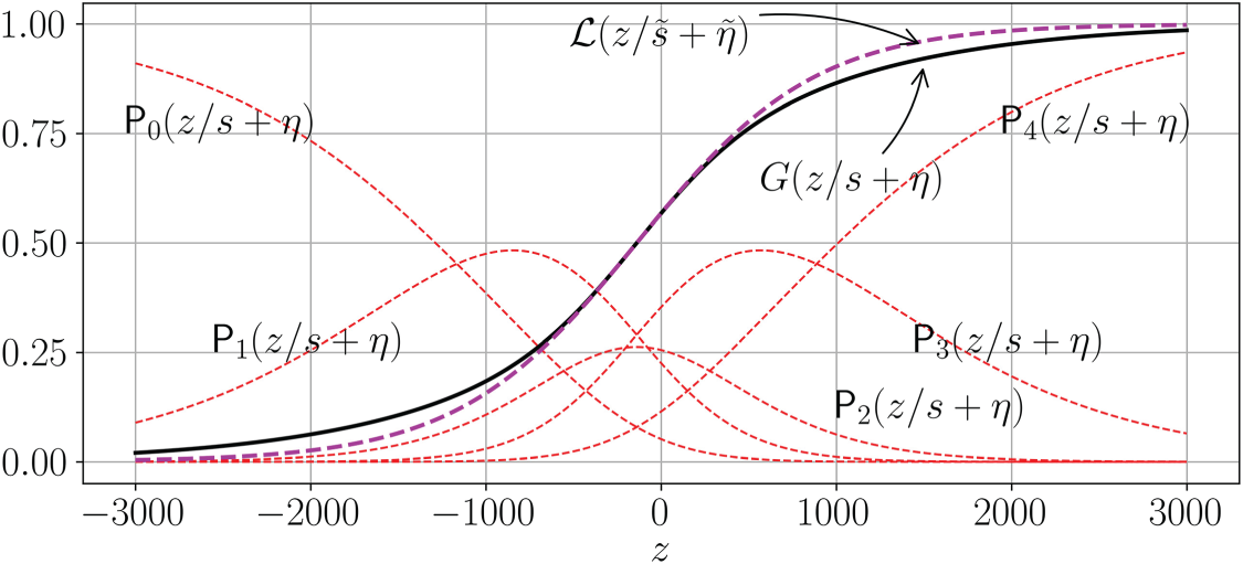
To illustrate how this works for $L = 5$ , we have shown the approximation $L (z / \tilde{s} + \tilde{η})$ in Figure 3, while the common case of the three-level outcomes is discussed in the following example.

Example 3 (

L = 3

In games with three-level outcomes, i.e., when $L = 3$ , $δ = [0, 0.5, 1]$ and $α = [0, α_{1}, 0]$ , we have

β_{AC \to L} = 1 + 0.5 e^{α_{1}},

(94)

and the approximation results are shown in Figure 4 for different values of

α_{1}

. From Proposition 2 we know that for

α_{1} \approx 0.7

, we have

β_{AC \to L} = 2

and

G (z / s) = L (z / \tilde{s})

, i.e., there is no approximation error.

Figure 4.

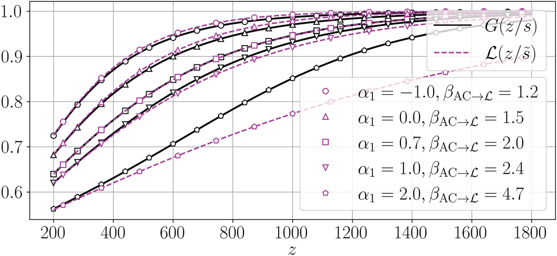
Comparison between $G (z / s)$ and its approximation $L (z / \tilde{s})$ , for $L = 3$ , $\tilde{s} = s β_{AC \to L}$ , $β_{AC \to L}$ given in (94), $δ = [0, 0.5, 1]$ , $α = [0, α_{1}, 0]$ , where the values of $α_{1}$ are given in the legend; $s = 174$ . For smaller values of $z$ , the curves practically superimpose. For $α_{1} = \log 2 \approx 0.7$ , we have a true equivalence of the expected scores, i.e., $G (z / s) = L (z / \tilde{s})$ , where $\tilde{s} = 2 s$ .

Although Figure 4 provides us with a cautionary note about the model mismatch, it seems to be important only for large $α_{1}$ , say $α_{1} \geq 0.7$ . Thus, the question is whether such models are suitable for describing the results of the matches?

This can be answered using data, but a glimpse of insight may be obtained assuming that all skills are comparable and thus $z_{t} \approx 0$ (as may happen, with small $v_{θ}$ , e.g., in the league competitions), so we can find the probability of the draw as (see also Szczecinski and Djebbi (2020: Eq. (47)))

P_{1} (z) |_{z \approx 0} \approx \frac{e^{α_{1}}}{2 + e^{α_{1}}}

(95)

Then, for $α_{1} = - 1.0, 0.0, 0.7, 1, 2$ , which we used in Figure 4, we obtain, respectively, the probability of the draw (95) $\approx 0.16, 0.33, 0.5, 0.58, 0.79$ .

The probability of the draw larger than 0.5 (i.e., for $α_{1} > 0.7$ , where the mismatch is apparent in Figure 4) seems rather unlikely in popular sports with three level outcomes, such a football, basketball. Then, we would rather use $α_{1} < 0.7$ and the Elo algorithm’s $L (z / \tilde{s})$ is a reasonable approximation of the expected score $G^{AC} (z / s)$ . In competition where large $α_{1}$ makes sense (e.g., in chess, the probability of draws may be large) the modeling mismatch will be more important.

Cumulative Link model

The CL model is defined as (Tutz, 2012: Ch. 9.1)

P_{y} (z) = L (z - c_{y - 1}) - L (z - c_{y}),

(96)

where the model’s thresholds are monotonically increasing, i.e.,

c_{y} > c_{y - 1}

, we set

c_{- 1} = - \infty

and

c_{L - 1} = + \infty

, and the symmetry condition (7) is satisfied by

c_{y} = - c_{L - 2 - y}, y = 0, \dots, L - 2;

(97)

for

L

even, (97) implies

c_{L / 2 - 1} = 0

. The thresholds are collected in

c = [c_{0}, \dots, c_{L - 2}]

ML+SG Ranking

To obtain the ranking algorithm, we calculate the log-likelihood and its derivative

ℓ_{y} (z) = \log (e^{c_{y} - c_{y - 1}} - 1) - \log (1 + e^{z - c_{y - 1}}) - \log (1 + e^{c_{y} - z}),

(98)

{\dot{ℓ}}_{y} (z) = L (c_{y} - z) - L (z - c_{y - 1}),

(99)

which, used in the ranking update (12), becomes

θ_{t + 1} = θ_{t} + μ x_{t} [L (c_{y_{t}} - z_{t} / s) - L (z_{t} / s - c_{y_{t} - 1})],

(100)

generalizing the formula shown in Lasek and Gagolewski (2021: Sec. 2.2). However, we are not aware of any ranking based on the simple update (100).

For $L = 2$ , (100) is equivalent to the Elo ranking with binary outcomes (22); for $L > 2$ the update (100) will never be identical to the multilevel Elo ranking (64). This aspect alone, although it does not disqualify the CL model, makes the latter less natural when analysing the Elo ranking – which is why we focus on the AC model in Section “Decoupling prediction from ranking” and use the CL model only as a baseline in Example 6.

We can also replace the logistic function $L (z)$ in (96) with the Gaussian CDF, $Φ (z)$ ; this is done in the FIVB ranking which uses $L = 6$ with thresholds $c_{0} = - 1.06$ , $c_{1} = - 0.394$ , $c_{2} = 0$ (others by symmetry (97)). However, the equations for ${\dot{ℓ}}_{y} (z)$ are not as simple as (99) and require some implementation care (Tenni et al., 2025: Sec. 2.5).

Decoupling prediction from ranking

We have shown that the Elo algorithm implicitly optimizes the AC model when scores are uniform, but that the implicit model parameters need not match the data. Since our goal is not to change the Elo algorithm but to provide statistical tools to evaluate its performance and interpret its results, we decouple estimation from prediction: the Elo algorithm continues to produce $θ_{t}$ as before, while the prediction model is an AC model parameterized by $(\hat{δ}, \hat{α}, \hat{η}, \hat{β})$ , fitted to the outcomes $y_{t}$ and to the estimated skill differences $z_{t} = x_{t}^{T} θ_{t}$ produced by ranking:

\hat{δ}, \hat{α}, \hat{η}, \hat{γ} = \underset{δ, α, η, γ}{argmax} \sum_{t \in T^{train}} ℓ_{y_{t}} (γ z_{t} / s + η h_{t}; δ, α),

(101)

\hat{β} = 1 / \hat{γ} .

(102)

We use

γ = 1 / β

to guarantee concavity and thus uniqueness of the solution; for fixed

δ

the objective is jointly concave in

α

η

, and

γ

, and concave in

δ

for fixed

γ

α

η

. Alternate optimization over these blocks is therefore convergence-safe.

The scale adjustment $\hat{β} = 1 / \hat{γ}$ plays a double role: it aligns the expected score of the AC model with that of the Elo algorithm (through $β_{AC \to L}$ , see (92)), and it corrects for estimation noise and pre-convergence compression as $β_{err}$ did in the binary case (60). These two effects are entangled and handled jointly by fitting $\hat{γ}$ from data, making analytical disentanglement unnecessary in practice.

Avoiding optimization

Instead of the full optimization (101), three closed-form initializations suffice in practice, obtained by (a) borrowing scores from the Elo algorithm and (b) exploiting the approximation $z_{t} \approx 0$ (reasonable when skill dispersion is small relative to the scale, e.g., in balanced league competition):

Scores $\hat{δ}$ : We set $\hat{δ} = ρ$ , borrowing the scores used in the Elo algorithm. This is motivated by the structural similarity between Elo (64) and G-Elo (84).

Parameters $\hat{α}$ : Setting $z_{t} = 0$ and $η = 0$ , (101) reduces to

\hat{α} = \underset{α}{argmax} \sum_{y \in Y} {\bar{P}}_{y} \log P_{y} (0),

(103)

where

P_{y} (0) = e^{α_{y}} / \sum_{l} e^{α_{l}}

and where

{\bar{P}}_{y}

are the observed outcome frequencies in

T^{train}

. Symmetrization

{\bar{P}}_{y}^{sym} = \frac{1}{2} ({\bar{P}}_{y} + {\bar{P}}_{L - 1 - y})

enforces (77), after which the constraint

{\hat{α}}_{y} = {\hat{α}}_{L - 1 - y}

is automatically satisfied and (103) yields

e^{{\hat{α}}_{y}} \propto {\bar{P}}_{y}^{sym},

(104)

{\hat{α}}_{y} = \log \frac{{\bar{P}}_{y}^{sym}}{{\bar{P}}_{0}^{sym}},

(105)

where division by

{\bar{P}}_{0}^{sym}

enforces

α_{0} = α_{L - 1} = 0

, (79).

Home-field advantage $\hat{η}$ : With $z_{t} = 0$ and $\hat{α}$ fixed, the objective (101) over matches with $h_{t} = 1$ reduces to

\hat{η} = \underset{η}{argmax} \sum_{y \in Y} {\bar{P}}_{y, hfa} \log P_{y} (η),

(106)

where

{\bar{P}}_{y, hfa}

is the frequency of outcome

y

in home-venue matches in

T^{train}

. Setting the derivative to zero yields

G^{AC} (\hat{η}) = {\bar{δ}}_{hfa},

(107)

{\bar{δ}}_{hfa} = \sum_{y \in Y} {\bar{P}}_{y, hfa} δ_{y},

(108)

which is solved numerically or, using

G^{AC} (z) \approx L (z / β_{AC \to L})

from (93), in closed form as

\hat{η} \approx β_{AC \to L} \log \frac{{\bar{δ}}_{hfa}}{1 - {\bar{δ}}_{hfa}} .

(109)

Scale adjustment $\hat{β}$ : Using only model equivalence and ignoring estimation noise gives

{\hat{β}}_{0} = 1 / β_{AC \to L},

(110)

which is the only sensible choice when

z_{t} \approx 0

. When the skill differences

z_{t}

are informative,

\hat{β}

is refined by solving (101) with fixed

\hat{α}

\hat{η}

\hat{δ}

. Then

{\hat{β}}_{0}

has a diagnostic role:

\hat{β} < {\hat{β}}_{0}

indicates compressed skill differences, i.e., lack of convergence.

As we shall see in Examples 4–5, these simple formulas already capture most of the prediction gain; the only parameter that benefits from further data-driven refinement is $\hat{β}$ .

We briefly note that the strategy of using $z_{t} \approx 0$ can also be applied to initialize $\hat{δ}$ (by jointly optimizing over $δ$ and $η$ using the frequency of outcomes at the home-venue), but reusing $\hat{δ} = ρ$ is a robust alternative that we recommend.

Closed-form initializations (105), (109), and (110) can be used directly in (61) adapted to the AC model:

L S = - \frac{1}{| T^{test} |} \sum_{t \in T^{test}} ℓ_{y_{t}} (\frac{z_{t}}{s \hat{β}} + \hat{η} h_{t}; \hat{δ}, \hat{α}),

(111)

where

T^{test}

contains the indices of matches played after those in the training set.¹⁶

We also calculate the ranked probability score (RPS) which is a performance metric specialized in dealing with ordinal outcomes and defined as follows (Constantinou and Fenton, 2012):

R P S = \frac{1}{| T^{test} |} \sum_{t \in T^{test}} {R P S}_{t},

(112)

{R P S}_{t} = \frac{1}{L - 1} \sum_{y = 0}^{L - 2} {(F_{y} - I [y_{t} \leq y])}^{2},

(113)

where

F_{y} \equiv \sum_{k = 0}^{y} P_{k} (\frac{z_{t}}{s \hat{β}} + \hat{η} h_{t}; \hat{δ}, \hat{α})

is the predicted cumulative probability. Unlike the log-score, RPS takes into account the predictions for all outcomes and is less sensitive to the over-confindent predictions.

Example 4 (Pseudo-model identification).

For $θ *$ we used in Example 1 we generate the outcomes of the matches using the AC model (76) with $L = 3$ , and parameters $η * = 0.35$ and $α_{1} * = - 0.4$ (of course, $δ *_{1} = 0.5$ ). We use the Elo algorithm (22) with scale $s = 174$ , $η = 0$ , $ρ_{1} = 0.5$ , and steps $K = 20$ and $K = 60$ .

We define the set $T^{train} = {4000, \dots, 7999}$ for pseudo-model identification in (101), and a testing set $T^{test} = {8000, \dots, 12000}$ for evaluation in (111). The matches indexed with $t < 4000$ are only used to ensure convergence. The frequency ${\bar{P}}_{y}$ needed in (105)–(110) is estimated from the outcomes $y_{t}, t \in T^{train}$ .

To assess the benefit of full adaptation (101) relative to non-adaptive methods, we consider the following cases, ordered by increasing use of data and/or prior information:

Conventional: Based on the premise that the model used in ranking must be used for prediction, we use $\hat{η} = 0$ , ${\hat{α}}_{1} = \log 2 \approx 0.7$ , and $\hat{β} = 1 / β_{AC \to L} = 0.5$ , as implied by Proposition 2. This illustrates the “coupling” of the models which ignores model mismatch (as well as the estimation noise); it is a “straw man” baseline, also used in Szczecinski and Roatis (2022).

Initialization, no HFA: ${\hat{α}}_{1}$ from (105), $\hat{β} = {\hat{β}}_{0}$ , (110), and $\hat{η} = 0$ . This is done to verify how much we lose by ignoring the HFA in the performance evaluation.

Initialization, with HFA: as above, and $\hat{η}$ is calculated from (109).

Initialization, optimal scaling: $\hat{β}$ is found solving (101) under constraints of fixed ${\hat{α}}_{1}$ and $\hat{η}$ obtained from (105)-(109).

Fully adaptive: $\hat{α}$ , $\hat{η}$ and $\hat{β}$ are found from (101).

G-Elo: The results of the G-Elo algorithm (84) with values $α *_{1}$ and $η *$ are used to calculate the log-score (111) with $\hat{η} = η *$ and ${\hat{α}}_{1} = α_{1} *$ . Due to the perfect alignment of the models used in data generation, ranking, and prediction, $\hat{β} > 1$ appears to only correct for the presence of estimation noise, i.e., $\hat{β} \approx β_{err}$ .

In Table 2 we compare the log-score (111) and RPS (112) of the methods listed above against the lower bound of the ground-truth which no data-driven method can surpass.¹⁷ When

{\hat{α}}_{1}

\hat{η}

\hat{β}

are estimated from the data, we show (mean, standard deviation) over

J = 200

realizations.

Table 2.
Log-score (111) and RPS (112), ${\hat{α}}_{1}$ , $\hat{β}$ , and $\hat{η}$ for ternary matches with true parameters $α _{1} = - 0.4$ , $η = 0.35$ . Elo runs with the scale $s = 174$ , and two values of $K$ . Lower values of $L S$ and $R P S$ indicate better prediction. When obtained from the data, we show mean $\pm$ std obtained from $J = 200$ realizations; numbers without $\pm$ are predefined values or RPS which has negligible variation.

Method	${\hat{α}}_{1}$	$\hat{β}$	$\hat{η}$	$L S$	$R P S$
$K = 20$
Conventional	$0.69$	$0.50$	$0$	$1.12 \pm 0.01$	$0.22$
Init., no HFA	$- 0.53 \pm 0.04$	$0.77 \pm 0.01$	$0$	$1.00 \pm 0.01$	$0.21$
Init., with HFA			$0.29 \pm 0.04$	$0.99 \pm 0.01$	$0.21$
Init., opt. scaling		$0.89 \pm 0.02$		$0.99 \pm 0.01$	$0.21$
Fully adaptive	$- 0.42 \pm 0.04$	$0.86 \pm 0.02$	$0.34 \pm 0.04$	$0.99 \pm 0.01$	$0.21$
G-Elo	$α *_{1}$	$1.12 \pm 0.03$	$η *$	$0.98 \pm 0.01$	$0.21$
$K = 60$
Conventional	$0.69$	$0.50$	$0$	$1.16 \pm 0.01$	$0.23$
Init., no HFA	$- 0.53 \pm 0.04$	$0.77 \pm 0.01$	$0$	$1.03 \pm 0.01$	$0.22$
Init., with HFA			$0.29 \pm 0.04$	$1.02 \pm 0.01$	$0.22$
Init., opt. scaling		$1.18 \pm 0.03$		$1.00 \pm 0.01$	$0.21$
Fully adaptive	$- 0.44 \pm 0.04$	$1.16 \pm 0.04$	$0.33 \pm 0.04$	$1.00 \pm 0.01$	$0.21$
G-Elo	$α *_{1}$	$1.40 \pm 0.03$	$η *$	$1.00 \pm 0.01$	$0.21$
Ground truth ( $z *_{t}$ )	$α_{1} *$	$1$	$η *$	$0.98 \pm 0.01$	$0.20$

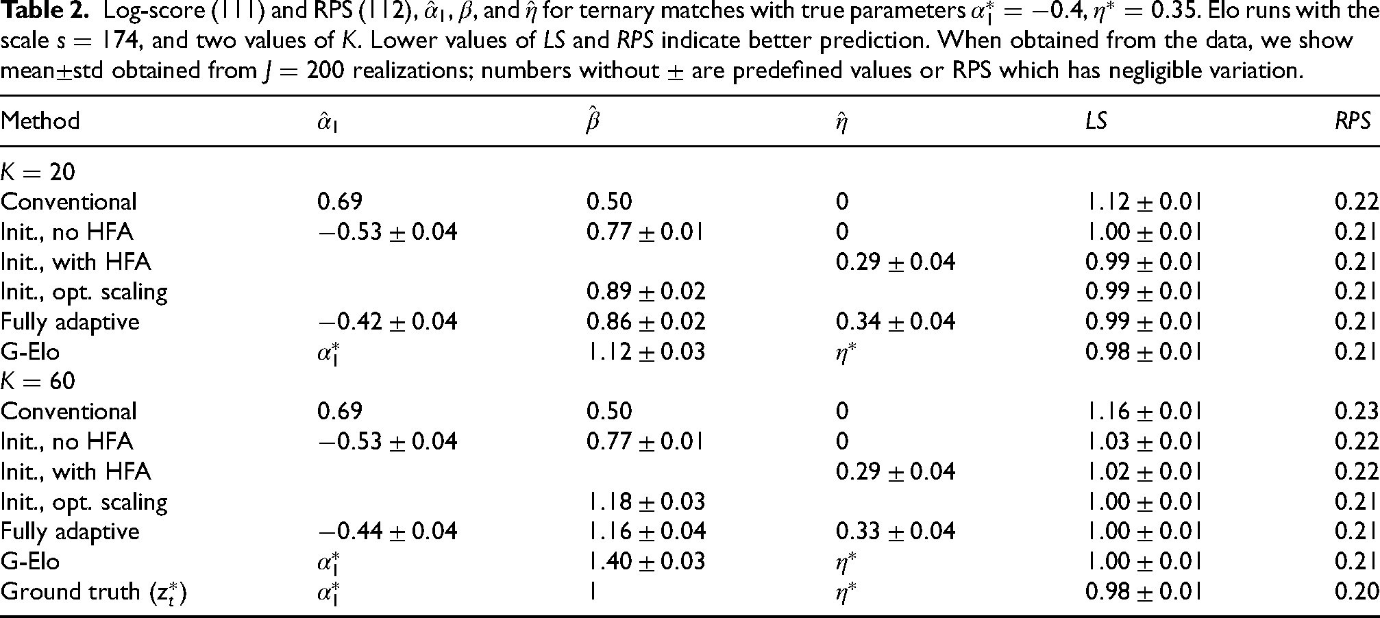
We conclude that:

Model decoupling pays off: the conventional (coupled) baseline yields the worst scores by far – confirming that blindly reusing the ranking model for prediction is harmful regardless of the estimation noise level. Both $L S$ and $R P S$ tell the same story, with the relative ordering of the methods identical for both metrics. The $L S$ gaps are proportionally larger, reflecting its greater sensitivity to overconfident predictions.

HFA recovery yields a small but consistent gain: accounting for $\hat{η}$ improves both scores at all noise levels. For small estimation noise ( $K = 20$ ), simple closed-form estimates already recover near-ground truth performance despite the Elo algorithm having completely ignored HFA.

Re-scaling is important: $\hat{β}$ increases from $\approx 0.89$ (at $K = 20$ ) to $\approx 1.18$ (for $K = 60$ ), reflecting the inflation scaling due to estimation noise consistent with the binary case. With ${\hat{α}}_{1}$ and $\hat{η}$ set by (105)–(109), adapting $\hat{β}$ alone from the data suffices; the fully adaptive approach does not provide a meaningful additional gain.

Exact modeling is not necessary for ranking: the scores based on the Elo algorithm are within one standard deviation of those of the G-Elo algorithm (which uses the correct model for ranking). This suggests that the gains reported by Szczecinski (2022), Szczecinski and Roatis (2022) were mainly due to the use of the AC model for performance evaluation and much less due to the ranking algorithm itself.

On-line adaptation

Instead of (101), and more in the on-line spirit of the Elo ranking, we may solve the problem using an on-line mini-batch approach, e.g., for $β_{t} = 1 / γ_{t}$ :

γ_{t + 1} = γ_{t} + \frac{μ_{γ}}{| T_{t} |} \sum_{τ \in T_{t}} \frac{d}{d γ} ℓ_{y_{τ}} (γ z_{τ} / s + \hat{η}; \hat{α}) |_{γ = γ_{t}}

(114)

= γ_{t} + \frac{μ_{γ}}{| T_{t} |} \sum_{τ \in T_{t}} \frac{z_{τ}}{s} (δ_{y_{τ}} - G^{AC} (γ_{t} z_{τ} / s + \hat{η}; \hat{α}))

(115)

where

μ_{γ}

is the adaptation step, and

T_{t} = {t - W + 1, \dots, t}

is the length-

W

mini-batch of indices.¹⁸ which should be chosen to average out the randomness in the gradients but preserve adaptability; for long competitions it may be at the order of hundreds. Note that we use

\hat{α}

and

\hat{η}

obtained via (105) and (109), which we have already found to perform well. Their on-line adaptation is possible, but we have not found it useful.

Example 5 (FIFA Men’s ranking).

Let us consider $T = 5719$ FIFA international Men’s teams matches played from 2018 $-$ 06 $-$ 04 to 2024 $-$ 07 $-$ 14, recovered from Football Rankings (2026) with given $y_{t}$ and $θ_{t, m}$ . The FIFA Elo-style algorithm has expected score $L (z / s; 10)$ with $s = 600$ , which corresponds to using $L (z / \tilde{s})$ with $\tilde{s} = s β_{10 \to e} = s / \log 10 \approx 260.6$ . The HFA indicators $h_{t}$ are found analyzing the data from soc (2026) and using AI tools (Anthropic, 2026).

We do not need to know how the results and/or skills were obtained (penalties, overtime, forfeit, initialization), which is in line with our model decoupling strategy: what matters is how to fit the pseudo-model for performance identification.

We set $T^{train} = {T^{'}, \dots, T^{″} - 1}$ , $T^{test} = {T^{″}, \dots, T}$ , with $T^{'} = 2000$ , $T^{″} = 4000$ . The frequency ${\bar{P}}_{y}$ needed in (105)–(110) is estimated from the outcomes $y_{t}, t \in T^{train}$ . We compare the following methods:

Worst case ( $z_{t} = 0$ ): prediction of the training outcome frequencies ${\bar{P}}_{y}$ alone, ignoring skill differences by setting $z_{t} = 0$ . This establishes a baseline that uses no ranking information. The parameters are not displayed, even though the probabilities are encoded in the model (via ${\hat{α}}_{1}$ and $\hat{η}$ ).

Conventional: based on the premise that the model used in the ranking must be used for the prediction, we use $\hat{η} = 0$ , ${\hat{α}}_{1} = \log 2 \approx 0.693$ , and $\hat{β} = 1 / β_{AC \to L} = 0.5$ , as implied by Proposition 2. This is the “straw man” baseline that ignores model mismatch and estimation noise.

Initialization, no HFA: ${\hat{α}}_{1}$ from (105) and $\hat{β} = {\hat{β}}_{0}$ from (110), $\hat{η} = 0$ .

Initialization, with HFA: ${\hat{α}}_{1}$ from (105) and $\hat{β} = {\hat{β}}_{0}$ from (110), $\hat{η}$ from (109).

Initialization, optimal scaling: ${\hat{α}}_{1}$ from (105), $\hat{η}$ from (109), $\hat{β}$ optimized through (101) with fixed ${\hat{α}}_{1}$ and $\hat{η}$ .

On-line adaptive: ${\hat{α}}_{1}$ from (105), $\hat{η}$ from (109), $\hat{β}$ is tracked in real time via (114) and reported as its mean over $T^{test}$ .

Fully adaptive: $\hat{α}$ , $\hat{η}$ , and $\hat{β}$ are found jointly from (101).

The 95% confidence interval (CI) on the parameters and on

L S

are obtained by resampling the training set

1000

times with replacement, re-deriving/optimizing all parameters from each resample, and evaluating the scores on the fixed test set. We do not show CI when the parameters are fixed by definition or when the RPS variation is negligible. The results are shown in Table 3.

Table 3.
Log-score (111) and RPS (112), ${\hat{α}}_{1}$ , $\hat{β}$ , and $\hat{η}$ for FIFA men’s international matches ( $T = 5719$ games, $2018 - 06 - 04 \to 2024 - 07 - 14$ ); $T^{train}$ : ( $2020 - 11 - 16 \to 2022 - 11 - 17$ ); $T^{test}$ : ( $2022 - 11 - 17 \to 2024 - 07 - 14$ ). Elo uses $\tilde{s} = s / \log 10 \approx 260.6$ (FIFA $s = 600$ and $L (\cdot; 10)$ ). Lower $L S$ and $R P S$ are better. 95% bootstrap CI are shown in brackets but for (i) fixed parameters, (ii) RPS which has negligible variation, and (iii) the on-line estimation where the bootstrap is not applicable because $β_{t}$ depends on the order of the outcomes.

Method	${\hat{α}}_{1}$	$\hat{β}$	$\hat{η}$	$L S$	$R P S$
Worst case ( $z_{t} = 0$ )	–	–	–	$1.040 [1.039, 1.042]$	$0.23$
Conventional	$0.69$	$0.50$	$0.00$	$0.998$	$0.20$
Init., no HFA	$- 0.59 [- 0.69, - 0.49]$	$0.78 [0.76, 0.80]$	$0$	$0.904 [0.902, 0.907]$	$0.18$
Init., with HFA			$0.73 [0.61, 0.87]$	$0.895 [0.892, 0.899]$	$0.18$
Init., opt. scaling		$0.54 [0.50, 0.59]$		$0.894 [0.889, 0.900]$	$0.18$
Init., on-line (114)	$- 0.59$	$0.60$	$0.73$	$0.890$	$0.18$
Fully adaptive	$- 0.30 [- 0.42, - 0.19]$	$0.50 [0.45, 0.55]$	$0.83 [0.68, 1.00]$	$0.892 [0.888, 0.899]$	$0.18$

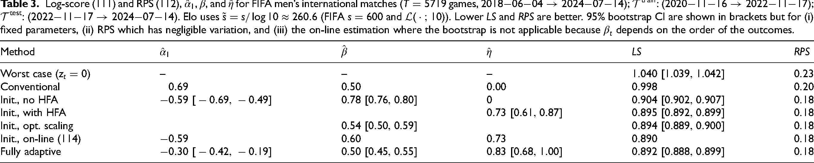
We observe that:

Predictive power: all skill-based methods outperform the worst case by a meaningful margin.

Results in line with synthetic case: the conventional approach straw-mans the FIFA ranking and we can do much better using simple formulas for $\hat{α}$ and $\hat{η}$ in (105) and (109);

Full adaptation is not required.

Optimal scaling: $\hat{β} = 0.541$ is smaller than the simple initialization $\hat{β} = 0.783$ from (110), reflecting the pre-convergence compression of skill differences already visible in Figure 5.

Figure 5.

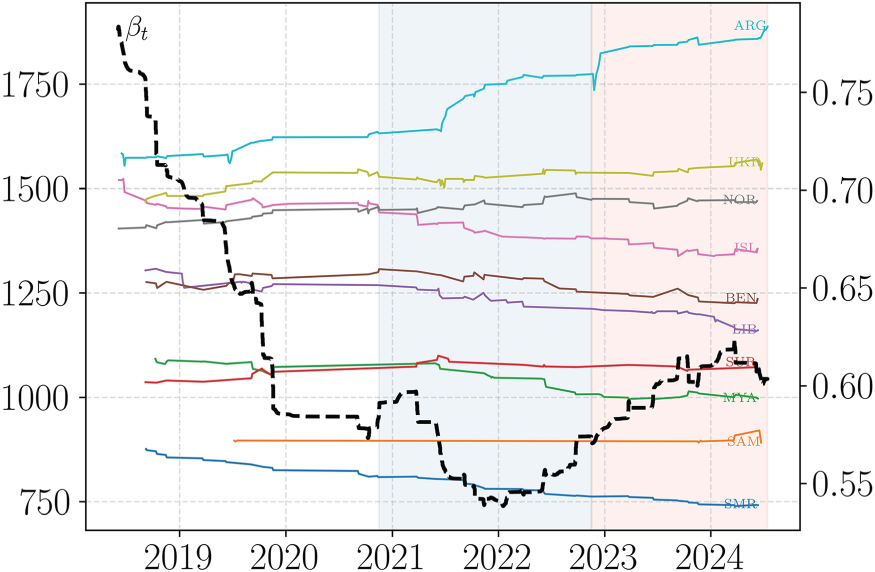
Skills (left axis) of the teams, from the best to the worst, (thin lines and three-letter abbreviations) and $β_{t}$ (dashed thick line) estimated via (114) (right scale). The shaded regions correspond to the training/testing sets (blue/rose, respectively).

Regarding the last observation, it is instructive to inspect $β_{t}$ obtained by (114) and shown in Figure 5 together with the skills of 10 teams covering uniformly the range of skill values at the end of data.

We can visually appreciate that the skills’ spread increases in time, i.e., we cannot declare convergence, and thus the skill differences are too small compared to those at the hypothetical convergence. This observation, already made in Szczecinski and Roatis (2022: Sec. 5.1), is more accurately assessed by $β_{t}$ : since $\hat{β} < 1$ , the scale adjustment amplifies the compressed skill differences.

The lack of convergence can be well explained by analyzing how many time-constants each team $m$ has accumulated on average, i.e., we calculate the exponent in (45)

Λ_{m} = \frac{N_{m}}{{\bar{τ}}_{m}},

(116)

where

N_{m}

is the number of matches played by team

m

and

{\bar{τ}}_{m}

is given in (47). The cumulative distribution of

Λ_{m}

is shown in Figure 6 where, by 2020, none of the teams had accumulated even one time constant; clearly, no convergence could be declared in its most liberal interpretation.

Figure 6.

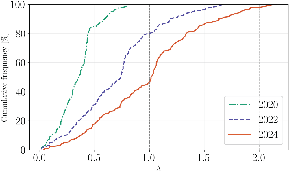
Percentage of international FIFA teams which have played at least $Λ_{m} = Λ$ time constants worth of matches by the year 2020, 2022, and 2024. The vertical lines indicate $Λ = 1$ and $Λ = 2$ ; $Λ \approx 2$ is required to reliably declare convergence in the mean.

Since 2022, the convergence conditions improve (note also the increase in $β_{t}$ in Figure 5), yet by 2024, 80% of the teams have not played enough matches to accumulate one time constant ${\bar{τ}}_{m}$ , and 98% of teams have fewer matches than $2 {\bar{τ}}_{m}$ . After six years of running the algorithm, convergence cannot be declared yet. This happens mainly because weak teams do not qualify for high-stakes matches (where $K_{t}$ is large) and play a small number of matches with slow convergence, e.g., friendlies with $K_{t} \in {5, 10}$ .

Example 6 (Decoupling beyond Elo).

To illustrate how the decoupling principle applies in a general case (that is, irrespectively of whether the Elo algorithm is used for the ranking), we consider the FIVB Men’s volleyball ranking (FIVB, 2024; Tenni et al., 2025), which uses a CL-based ranking algorithm with scale $s = 125$ and $L = 6$ ordered outcomes: $y = 0$ (away win $0$ - $3$ ), $y = 1$ ( $1$ - $3$ ), $y = 2$ ( $2$ - $3$ ), $y = 3$ ( $3$ - $2$ ), $y = 4$ ( $3$ - $1$ ), and $y = 5$ (home win $3$ - $0$ ). From the decoupling perspective, the details of the ranking algorithm do not matter: the estimated skills $z_{t} = θ_{t, home} - θ_{t, away}$ are given (at the FIVB website), and we focus on fitting a prediction model. The matches are split by year into a training set (2021–2023) and a test set (2024–2025). Since venue information is not available, we set $η = 0$ throughout.

Although we can choose any model, we decide to use the AC model as this illustrates the best the decoupling idea; the CL model is only used as a baseline and in a simple adaptation of the scale. We compare the following methods:

Worst case ( $z_{t} = 0$ ): as in Example 5, we ignore the skills but the prior probabilities ${\bar{P}}_{y}$ are captured in the AC model via $\hat{α}$ initialized from the training outcome frequencies.

FIVB baseline: the CL model (96) with thresholds $c_{0} = - 1.06$ , $c_{1} = - 0.394$ (others by symmetry (97)), and scale $s = 125$ , all defined by FIVB; no parameters are optimized. Unlike the FIFA case, the FIVB explicitly defines the multilevel model $P_{y} (z)$ used for prediction.

FIVB + scale: as above, but the effective scale $\hat{β}$ is fitted on the training set with $c_{y}$ fixed.

AC optimal: $\hat{δ} = [0, {\hat{δ}}_{1}, {\hat{δ}}_{2}, 1 - {\hat{δ}}_{2}, 1 - {\hat{δ}}_{1}, 1]$ , $\hat{α} = [0, {\hat{α}}_{1}, {\hat{α}}_{2}, {\hat{α}}_{2}, {\hat{α}}_{1}, 0]$ , and $\hat{γ}$ are optimized jointly on the training set, subject to the symmetry constraints (77)–(79).

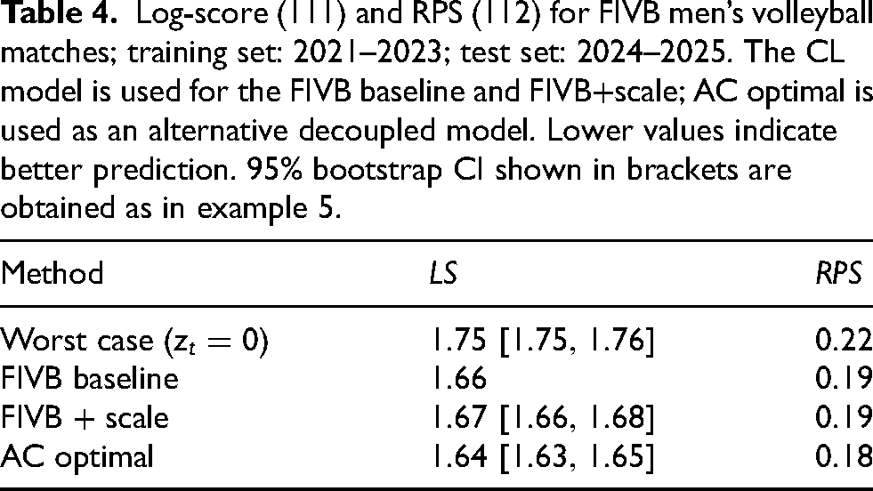
The scores are shown in Table 4 and we conclude that:

The decoupling works: for prediction, the CL model can be replaced by the AC model which produces better scores than both FIVB baselines, despite using a fundamentally different model family.

Convergence: we found the CI for $\hat{β}$ equal to $[0.74, 0.97]$ and no meaningful improvement is obtained via scaling. This means that the algorithm almost converged; this is a much better situation than in the FIFA ranking.

AC model: In the optimized AC predictor we obtained ${\hat{δ}}_{1} = 0.19$ and ${\hat{δ}}_{2} = 0.39$ , which corresponds to a practically uniform distribution. This indicates that uniform scores ( $ρ_{y} = y / 5$ ) might be used if the Elo ranking (22) was to replace the current FIVB algorithm. However, the best course of action would be to fit the AC model to the data.

Table 4.

Log-score (111) and RPS (112) for FIVB men’s volleyball matches; training set: 2021–2023; test set: 2024–2025. The CL model is used for the FIVB baseline and FIVB+scale; AC optimal is used as an alternative decoupled model. Lower values indicate better prediction. 95% bootstrap CI shown in brackets are obtained as in example 5.

Method	$L S$	$R P S$
Worst case ( $z_{t} = 0$ )	$1.75 [1.75, 1.76]$	$0.22$
FIVB baseline	$1.66$	$0.19$
FIVB + scale	$1.67 [1.66, 1.68]$	$0.19$
AC optimal	$1.64 [1.63, 1.65]$	$0.18$

Note that, in this case we cannot readily produce the estimates of time constants per team because the FIVB ranking is not using the Elo algorithm. Deriving those should be possible but would take us too far from the scope of this work.

Conclusions

This work reconciles the practitioner’s and statistician’s perspectives on the Elo ranking algorithm around two main contributions: practitioners obtain a principled framework for the performance evaluation of the algorithm, while statisticians may interpret it as an approximate ML estimation via SG updates.

We recapitulate our finding as follows:

Binary outcomes In the binary case (Section “Elo ranking in binary matches”), the practitioner’s update rule and the ML+SG algorithm coincide if and only if the expected score is the logistic function $L (z / s)$ (Section “Practitioner meets statistician”), which is thus the unique expected score endowed with a full probabilistic interpretation. The scale $s$ and step $K$ govern a fundamental trade-off: for fixed $s$ , increasing $K$ reduces the convergence time constant $τ = 4 s / K$ (46) at the cost of greater asymptotic estimation variance $\bar{v} = K s / 2$ . This trade-off should guide the parameter choices in practice. The HFA parameter $η$ does not change if we rescale the skills (for a given expected score), and may be reused in different approximations of $L (z)$ if the product $η s$ is kept constant.

Estimation noise forces model decoupling. We show that the estimation noise produced by the SG algorithm forces a distinction between the ranking model and the prediction model even when both are otherwise identical. The effective scale used when predicting from the “noisy” estimated skills increases $\hat{s} = s β_{err} > s$ (58), while the effective HFA is attenuated $\hat{η} < η$ (59). A practitioner who reuses the nominal $s$ and $η$ for prediction systematically overestimates the predictive power of the model. The pseudo-model identification step (62) finds $\hat{s} = s \hat{β}$ and $\hat{η}$ directly from the data.

Multilevel outcomes. For $L > 2$ outcomes (Section “Beyond win/loss matches: Elo ranking for multilevel outcomes”), the G-Elo algorithm is the formal ML+SG update for the AC model. The Elo ranking with uniform scores ( $ρ_{y} = y / (L - 1)$ ) corresponds to G-Elo under the implicit AC model (Proposition 2). In general, the expected score $G^{AC} (z / s)$ and the logistic function $L (z / \tilde{s})$ agree only approximately. For $L = 3$ and draw probabilities typical in sports ( $α_{1} ≲ 0.7$ ) the approximation is accurate and Elo algorithm yields reasonable estimation results which explains why the algorithm “works” in practice.

Model decoupling in practice. The AC model parameters that correspond exactly to the Elo ranking need not be those that best describe the data. The decoupling principle (Section “Decoupling prediction from ranking”) resolves this by separating estimation from prediction: the parameters $(\hat{δ}, \hat{α}, \hat{η}, \hat{β})$ may be found from the data by treating the skills $θ_{t}$ as fixed inputs (101)–(111).

The examples on synthetic and FIFA data show that most of the gain is already captured by the simple closed-form estimates (105)–(110), with only $\hat{β}$ requiring data-driven refinement. The FIVB example further shows that the decoupling principle applies regardless of the ranking algorithm: replacing the CL-based FIVB model with a fitted AC model improves predictive performance, illustrating that the principle is not specific to the Elo algorithm.

The FIFA results emphasize the dual role of the scale parameter $\hat{β}$ : it corrects for the estimation noise (producing $\hat{β} > 1$ after convergence) and diagnoses lack of convergence ( $\hat{β} < 1$ when skill differences are compressed). The on-line estimate $β_{t}$ (114) tracks this in real time. The decoupling is conceptually transparent, computationally inexpensive, and consistently improves predictive performance.

Footnotes

Appendix A Derivation of ( 57 )

From (56), dropping the time-index $t$ , by the rule of multiplication of the Gaussian distributions Barber (2012: Sec. 8.4), we have (117)

f (z * | z) = N (z; z *, 2 \bar{v}) N (z *; 0, 2 v_{θ}) / N (z; 0, 2 (\bar{v} + v_{θ}))

(118)

= N (z *; z / a, 2 \bar{v} / a),

(119)

a = 1 + \bar{v} / v_{θ} .

Since we use $L (z / s + η) \approx Φ ((z + η s) / (s β_{L \to Φ}))$ , see (27), the following relationship is useful (120)

\int Φ ((x + z) / b) N (x; y, q^{2}) d x = Φ (\frac{y + z}{\sqrt{b^{2} + q^{2}}})

to express (55) as (121)

\bar{\Pr} {Y_{t} = 1 | z_{t}} \approx \int Φ (\frac{z * + η s}{s β_{L \to Φ}}) N (z *; \frac{z}{a}; 2 \frac{\bar{v}}{a}) d z *

(122)

= Φ (\frac{z / a + η s}{\sqrt{s^{2} β_{L \to Φ}^{2} + 2 \bar{v} / a}})

(123)

\approx L (\frac{z + η s a}{a \sqrt{s^{2} + 2 \bar{v} / (a β_{L \to Φ}^{2}})}) = L (\frac{z}{\hat{s}} + \hat{η}),

where

\hat{s}

is given in (58) and

\hat{η}

in (59).

Appendix B Proof of Proposition 2

Using the binomial expansion, $(1 + a)^{L - 1} =$ $\sum_{y = 0}^{L - 1} (\binom{L - 1}{y}) a^{y}$ , $α_{y} = \log (\binom{L - 1}{y})$ and $δ_{y} = \frac{y}{L - 1}$ , the expected score can be calculated as (124)

G (z / s) = \frac{\sum_{y = 0}^{L - 1} δ_{y} e^{α_{y} + δ_{y} z / s}}{\sum_{y = 0}^{L - 1} e^{α_{y} + δ_{y} z / s}} = \frac{\sum_{y = 1}^{L - 1} \frac{y}{L - 1} \frac{(L - 1)!}{y! (L - 1 - y)!} e^{z y / [s (L - 1)]}}{\sum_{y = 0}^{L - 1} (\binom{L - 1}{y}) e^{z y / [s (L - 1)]}}

(125)

= \frac{e^{z / [s (L - 1)]} \sum_{y = 0}^{L - 2} (\binom{L - 2}{y}) e^{z y / [s (L - 1)]}}{(1 + e^{z / [s (L - 1)]})^{L - 1}} = \frac{e^{z / [s (L - 1)]} (1 + e^{z / [s (L - 1)]})^{L - 2}}{(1 + e^{z / [s (L - 1)]})^{L - 1}}

(126)

= \frac{1}{1 + e^{- z / [s (L - 1)]}} = L (z / \tilde{s}) .

where

\tilde{s} = s (L - 1)

. This terminates the proof.

Funding

The author(s) received no financial support for the research, authorship, and/or publication of this article.

Declaration of interest statement

The authors declared no potential conflicts of interest with respect to the research, authorship, and publication of this article.

ORCID iD

Leszek Szczecinski

Notes

References

Aldous

(2017) Elo ratings and the sports model: A neglected topic in applied probability?. Statistical Science 32(4): 616–629.

Angelini

Candila

De Angelis

(2022) Weighted Elo rating for tennis match predictions. European Journal of Operational Research 297(1): 120–132.

Anthropic (2026) Claude. https://www.anthropic.com.

Barber

(2012) Bayesian Reasoning and Machine Learning. Cambridge University Press.

Brandes

Marmulla

Smokovic

(2025) Efficient computation of tournament winning probabilities. Journal of Sports Analytics 11: 22150218251313905. DOI: 10.1177/22150218251313905

Constantinou

Fenton

(2012) Solving the problem of inadequate scoring rules for assessing probabilistic football forecast models. Journal of Quantitative Analysis in Sports 8(1): 1–14.

Cortez

Tossounian

(2026) Convergence and stationary distribution of Elo rating systems. https://arxiv.org/abs/2410.09180.

Csató

(2023) Quantifying the unfairness of the 2018 FIFA world cup qualification. International Journal of Sports Science & Coaching 18(1): 183–196.

Csató

(2024) Club coefficients in the UEFA champions league: Time for shift to an elo-based formula. International Journal of Performance Analysis in Sport 24(2): 119–134.

10.

Darrell Bock

(1972) Estimating item parameters and latent ability when responses are scored in two or more nominal categories. Psychometrika 37(1): 29–51.

11.

Davidson

(1970) On extending the bradley-terry model to accommodate ties in paired comparison experiments. Journal of the American Statistical Association 65(329): 317–328.

12.

Davidson

Beaver

(1977) On extending the bradley-terry model to incorporate within-pair order effects. Biometrics 33(4): 693–702.

13.

Egidi

Ntzoufras

(2020) A Bayesian quest for finding a unified model for predicting volleyball games. Journal of the Royal Statistical Society Series C: Applied Statistics 69(5): 1307–1336.

14.

Egidi

Pauli

Torelli

(2018) Combining historical data and bookmakers’ odds in modelling football scores. Statistical Modelling 18(5-6): 436–459.

15.

Egidi

Torelli

(2021) Comparing goal-based and result-based approaches in modelling football outcomes. Social Indicators Research 156(2): 801–813.

16.

Elo

(1978) The Rating of Chessplayers, Past and Present. New York, NY, USA: Arco Publishing Inc.

17.

eloratingsnet (2020) World football Elo ratings. https://www.eloratings.net/.

18.

FIDE (2019) International chess federation: ratings change calculator. https://ratings.fide.com/calculator_rtd.phtml.

19.

FIFA (2018) Revision of the FIFA/Coca-Cola world ranking. https://digitalhub.fifa.com/m/f99da4f73212220/original/edbm045h0udbwkqew35a-pdf.pdf.

20.

FIVB (2024) Fivb volleyball world ranking. https://en.volleyballworld.com/volleyball/world-ranking/ranking-explained.

21.

FiveThirtyEight (2020) How our NFL predictions work. https://fivethirtyeight.com/methodology/how-our-nfl-predictions-work/.

22.

Football Rankings (2026) Football rankings. http://www.football-rankings.info/.

23.

Gelman

Hwang

Vehtari

(2014) Understanding predictive information criteria for Bayesian models. Statistics and Computing 24(6): 997–1016.

24.

Glickman

(1995) Chess rating systems. American Chess Journal 3: 59–102.

25.

Glickman

(1999) Parameter estimation in large dynamic paired comparison experiments. Journal of the Royal Statistical Society: Series C (Applied Statistics) 48(3): 377–394.

26.

Glickman

(2025) Paired comparison models with strength-dependent ties and order effects. https://arxiv.org/abs/2505.24783.

27.

Gomes de Pinho Zanco

Szczecinski

Vinicius Kuhn

, et al. (2024) Stochastic analysis of the Elo rating algorithm in round-robin tournaments. Digital Signal Processing 145: 104313.

28.

Hvattum

Arntzen

(2010) Using elo ratings for match result prediction in association football. International Journal of Forecasting 26(3): 460–470.

29.

Ingram

(2021) How to extend elo: A Bayesian perspective. Journal of Quantitative Analysis in Sports 17(3): 203–219.

30.

Jabin

Junca

(2015) A continuous model for ratings. SIAM Journal on Applied Mathematics 2(75): 420–442.

31.

Karlis

Ntzoufras

(2008) Bayesian modelling of football outcomes: Using the skellam’s distribution for the goal difference. IMA Journal of Management Mathematics 20(2): 133–145.

32.

Király

Qian

(2017) Modelling competitive sports: Bradley-terry-elo models for supervised and on-line learning of paired competition outcomes. arXiv e-prints: arXiv:1701.08055.

33.

Kovalchik

(2020) Extension of the elo rating system to margin of victory. International Journal of Forecasting 36(4): 1329–1341.

34.

Langville

Meyer

(2012) Who’s #1, The Science of Rating and Ranking. Princeton University Press.

35.

Lapré

Amato

(2025) The impact of imbalanced groups in uefa euro 1980–2024 and comparison with the fifa world cup. Journal of Quantitative Analysis in Sports. DOI: 10.1515/jqas-2024-0151.

36.

Lasek

Gagolewski

(2018) The efficacy of league formats in ranking teams. Statistical Modelling 18: 411–435.

37.

Lasek

Gagolewski

(2021) Interpretable sports team rating models based on the gradient descent algorithm. International Journal of Forecasting 37(3): 1061–1071.

38.

Lasek

Szlávik

Bhulai

(2013) The predictive power of ranking systems in association football. International Journal of Applied Pattern Recognition 1(1): 27–46.

39.

Morel-Balbi

Kirkley

(2025) Estimation of partial rankings from sparse, noisy comparisons. Communications Physics 9. DOI: 10.1038/s42005-025-02461-y.

40.

Newman

MEJ

(2023) Efficient computation of rankings from pairwise comparisons. Journal of Machine Learning Research 24(238): 1–25.

41.

Rao

Kupper

(1967) Ties in paired-comparison experiments: A generalization of the bradley-terry model. Journal of the American Statistical Association 62(317): 194–204.

42.

Soccerway (2026) Availabel at: https://www.soccerway.com (accessed 26 March 2026).

43.

Sonas

(2011) The Elo rating system – correcting the expectancy tables. Technical report.

44.

Szczecinski

(2022) G-elo: Generalization of the elo algorithm by modeling the discretized margin of victory. Journal of Quantitative Analysis in Sports 18(1): 1–14.

45.

Szczecinski

Djebbi

(2020) Understanding draws in Elo rating algorithm. Journal of Quantitative Analysis in Sports 16(3): 211–220.

46.

Szczecinski

Roatis

(2022) FIFA ranking: Evaluation and path forward. Journal of Sports Analytics 8(4): 231–250.

47.

Szczecinski

Tihon

(2023) Simplified kalman filter for online rating: One-fits-all approach. Journal of Quantitative Analysis in Sports 19(4): 295–315.

48.

Tang

Wang

Jin

(2025) Is Elo rating reliable? a study under model misspecification. https://arxiv.org/abs/2502.10985.

49.

Tenni

de Pinho Zanco

Szczecinski

(2025) FIVB ranking: Misstep in the right direction. Journal of Quantitative Analysis in Sports. DOI: https://doi.org/10.1515/jqas-2024-0128.

50.

Thurston

(1927) A law of comparative judgement. Psychological Review 34: 273–286.

51.

Tutz

(2012) Regression for Categorical Data. New York, NY, USA: Cambridge University Press.

52.

Tutz

(2020) A taxonomy of polytomous item response models. https://arxiv.org/abs/2010.01382.pdf.