The Recent Inflation Crisis and Long-run Economic Growth in India: An Empirical Survey of Threshold Level of Inflation

Abstract

This article investigates the existence of a threshold level of inflation and how any such level affects the growth of Indian economy. The article also seeks to examine the dynamic short-run and long-run relationship between inflation and economic growth in India. By employing spline regression method to estimate the threshold level of inflation and the long-run and short-run relationships, the results show a statistically significant structural break in the relationship between inflation and economic growth at 4 per cent. The study suggests that if inflation exceeds the threshold point, that is, 4 per cent, it will negatively affect economic growth. The autoregressive distributed lag (ARDL) model bound testing cointegration suggests that there are two cointegration vectors when gross domestic product and rate of interest are considered as the dependent variables. This result confirms the existence of the long-run equilibrium relationship between economic growth, inflation, exchange rate and rate of interest. From the long-run analysis, the study found that inflation is positively related to economic growth, whereas the other variables are not significant.

JEL Classification: E₄, E₆

Keywords

Inflation growth threshold level inflation causality Indian economy

Introduction

This article revolves around the estimation of the threshold level of inflation in Indian economy where the gross domestic product (GDP) is expected to grow at 7.5 per cent to 7.9 per cent in 2016–2017. This is a relevant issue to examine at this juncture because there is no such consensus readily available in the macroeconomic literature to support whether high inflation leads to high economic growth, low inflation leads to high economic growth or high inflation leads to slow economic growth, even though it is a well-established fact that some level of inflation is necessary for growth. Targeting inflation is one of the sole objectives of monetary policy of any country; however, the targeting of the inflation is based on whether the demand for money function is stable or not. In the wake of the 2008 subprime mortgage crisis, the US Federal Reserve bank used quantitative easing monetary policy to pump up dollars to revive the economy. However, a part of the overflow leaked into the emerging market economies and contributed towards increasing inflation there. Surprisingly, it did not lead to inflation in the United States. Rather, it helped to keep the interest rate low, which was expected to promote investment and consumption. On the contrary, inflation has also been low in Japan and Europe, leading to low growth. Even though Japan followed the US model of quantitative easing to lift its economy, it failed miserably because the stimulus has not been strong enough to push up the inflation. The European central bank has also declined the interest rate to increase the inflation and generate the domestic demand for goods. The danger of low inflation is that it slowly leads to recession, like slow poison, which was being experienced by the Japanese economy for a long period of time.

The principal objective behind raising inflation is to restore the economic growth. However, rising inflation not only disturbs the central bank of the nation in its attempt to sustain stable and low price as one of the central aims of the monetary policy but also has welfare cost of inevitable economic output. The causes that could be traced to why inflation inhibits growth, specifically to the Indian context, are probably the effects of inflation on the rate of investment. Rising rates of investment is necessary to meet the excess demand of a developing economy; however, inflation will hurt output growth through its effect on lowering the rate of investment. A major part of the population in India works in unorganized sectors and their wages are not indexed to inflation. As a result of which, the real disposable income decreases the total consumption and finally, reduce the growth as Indian economy is primarily driven by domestic demand. As a consequence of which, it surges openness of the economy and ever-growing requirements of investment. However, keeping in the mind the voluminous capital inflows into the Indian economy, it is important for the monetary policy authorities to address the necessary policy to curb high inflation.

In the light of the above, this article examined the possible existence of threshold inflation in the framework of growth–inflation relationship in the Indian context. Since last 30 months or so, inflation in India has kept policy makers off guard. In this circumstance, when the economy is on the path of recovering from worst hit financial crisis, where global and domestic demand are expected to register high growth and persistent inflation, it is a major concern for both the monetary policy and fiscal policy authorities. India’s key growth driver, corporate investment, is yet to catch the trends of investment for the period 2003–2008 where investment growth was around 16 per cent. This means that during 2008–2009 no industrial capacity has been created. Now, once the global and domestic demand will soar, investment has to upsurge, and this will further add burden to the existing high inflation in the upward direction. In this backdrop, it is essential to revisit the old question—What is the tolerable level of inflation for policy makers in India? This article is an endeavour in this direction.

At present there is no study, except those based on pooled data, which specifically investigates the issue of the relationship between inflation and economic growth and the question of a positive threshold in the Indian economy. The cross-country evidence of inflation and growth relationship shows that all the studies are based on the analysis till the 1990s. Moreover, a few studies have estimated the threshold level of inflation in the context of India. The present study found the research gap from a previous study by Singh and Kalirajan (2003) by providing an argument against the presence of some threshold level in India. The present study gives a clear picture of the existence of the threshold level of inflation in the context of India by using the monthly high- frequency data for the estimation and by adding some new explanatory variables for the threshold estimation. Additionally, this study is also trying to examine both the long-run and the short-run relationship between inflation and economic growth by employing the autoregressive distributed lag (ARDL) model bound test approach and unrestricted vector error correction model (VECM), which is the solitary contribution of this study to the existing literature.

The significance of the study is considered for the present condition of high and persistent level of inflation in the Indian economy. The study may help both monetary and fiscal policy authorities to stabilize the price level and its harmful effect on the growth level of Indian economy. The core contribution of this study is to estimate the threshold level of inflation, if any, in the context of India in order to understand the significance of tightening monetary policy to curb inflation. However, this study purposes to answer the following questions: (a) How inimical is inflation to economic growth? (b) How high or low should inflation rate be? and (c) What level of inflation affects the growth rate negatively?

This article is organized as follows: The review of literature is given in the second section, description of the variables and the period of study are considered in the third section. ‘Methodology: Threshold Model’ has been dealt in the fourth section. The empirical results are explained in the fifth section and the concluding remarks are given in the sixth section.

Review of Literature

In recent decades there have been extensive theoretical and empirical researches that examine the inflation growth trade-off. The findings of these existing research have been mixed and can be categorized into four possibilities. First, inflation has a neutral effect on growth (e.g., Cameron, Hum, & Simpson, 1998; Dorrance, 1963; Sidrauski, 1967). The second is that there is a positive relationship between inflation and economic growth (e.g., Mallick & Chodhury, 2001; Shi, 1999; Tobin, 1965). The third is that inflation has a negative effect on growth (e.g., Andres & Hernando, 1997; Barro, 1996; De Gregorio, 1992; Friedman, 1956; Gylfason, 1998, p. 21; Saeed, 2007; Stockman, 1981). Furthermore, Feldstein (1982) notes that ‘shifting the equilibrium rate of inflation one to zero percent would cause a continuous welfare gain equal to one percent of GDP a year’.

Empirical Evidence on the Inflation–Growth Relationship

In this section, the study provides a brief review of empirical literature that examined the relationship between inflation rates and economic growth and the notion of the nexus of negative inflation and growth. There is ample of literature on the inflation–growth relationship. To start with, the study provides a brief overview of the literature with focus on single-country analysis to determine whether there is a significant relationship between inflation and growth. The most celebrated method used to examine this relationship is the ordinary least squares (OLS) method (Bhatia, 1960; Lucas, 1973). The OLS is applied on pooled and cross section as well as time series regressions, and the R-squared value is used to indicate the strength of the relationship between inflation and growth. A few studies, however, have used more comprehensive multivariate models by regressing growth on inflation using a variety of explanatory variables. Naqvi and Khan (1989) explored the inflation and economic growth relationship in the context of Pakistan. The empirical results of the study suggest that Pakistan should keep inflation level of single digit and maintain a growth rate of GDP in the range of 6.5 to 7 per cent. The study also concluded that there is a negative relationship between inflation and economic growth in the context of Pakistan. Faria and Carneiro (2001) investigated the linkage between inflation and economic growth in the case of the Brazilian economy. They utilized the annual time series data covering the period from 1980 to 1995. By employing the bivariate time series technique, they found a short-run negative association between the variables. Sweidan (2004) investigated the nature of the economic growth and inflation relationship in Jordan for the time period 1970–2003. The findings show that there is a significant positive relationship between the two variables. However, a break point of 2 per cent is a threshold inflation level beyond which inflation affects growth negatively. Lee and Wong (2005) examined the threshold level inflation using quarterly data for 1965–2002 for Taiwan and 1970–2001 for Japan. The empirical findings suggest that an inflation rate beyond 7.25 per cent is detrimental for economic growth of Taiwan. In the context of Japan, they found two threshold points, one is 2.52 per cent and other is 9.66 per cent. This finding suggests that inflation rate below the threshold level is favourable to economic growth and beyond that it is detrimental to economic growth. Bhaduri (2007) analyzed the inflation and economic growth nexus from the perspective of Indian economy for the sample period 1976–2007. The empirical findings of the study show that a significant negative relationship exists between inflation and growth. This study also found that there is a persistent and strong negative relation between growth and inflation, while it is insignificant in the long run. Erbaykal and Okuyan (2008) examined the inflation and economic growth relationship in Turkey. To study the long-run relationship between the variables, they applied the bound testing methodology by Pesaran et al. (2001). They did not find a statistically long-run relationship, but they found a short-run relationship between inflation and economic growth. Munir, Mansur and Furuoka (2009) investigated the threshold level of inflation in the context of Malaysia by using the annual data covering the period 1970–2005. The findings reveal that inflation has no significant negative impact on the growth rate of GDP under the low inflation regime. This result also strongly suggests the coexistence of one threshold value beyond which inflation exerts a negative effect on economic growth. Mohanty, Chakraborty, Das and Jogn (2011) examined the existence of threshold effects between the inflation rate and economic growth in India, using the quaterly data Q₁: 1996–1997 to Q₃: 2010–2011. The empirical findings of the study suggest that there is a non-linear relationship between inflation and economic growth in India. The result also found that the threshold inflation level is between 4.0 and 5.5, which is statistically significant. On the one hand, the inflation growth literature shows strong evidence of a negative relationship between inflation and growth. On the other hand, there have been a few studies that reported a positive relationship between inflation and economic growth, regardless of the model or the control variables that are included in the model.

Cross-country Evidence on Inflation–Growth Relationship

Bhatia (1960) studied the relationship between inflation and economic growth in five developed countries, namely the United Kingdom (UK), Germany, Sweden, Canada and Japan. The study used a simple bivariate model by considering the rate of inflation and the growth rate. The study found the relationship between inflation and growth is inconclusive. Lucas (1973) investigated the relationship between inflation and economic growth. The study used a bivariate model by employing OLS. The study covered the period from 1951 to 1967 for 18 developing and developed countries. The result of the study suggests that there is a ‘stable trade-off between inflation and growth’. De Gregario (1992) examined 12 Latin American countries using data from 1950 to 1985. By using generalized least square (GLS) he found a negative relationship between inflation and growth. Stanner (1993) studied the inflation and economic growth relationship for 12 developed and developing countries. The study used the annual data covering the period from 1948 to 1986 and 1980 to 1988. The analysis used the simple correlation technique and found that low and zero inflation is an essential condition for high and sustained growth. De Gregorio (1996) revised the theory and evidence on inflation and growth and provided additional evidence on the non-linear relationship between the Organisation for Economic Co-operation and Development (OECD) and some developing countries in the period 1960–1985. He found a robust negative relationship between inflation and economic growth. He argued inflation limits growth mainly by reducing the efficiency of investment rather than its level. Paul, Kearney and Chowdhury (1997) investigated the inflation–growth relationship for 70 countries for the period 1960–1989. Their result shows absence of a causal relationship between inflation and economic growth in 40 per cent of the country. Consequently, in 20 per cent of the country they reported bidirectional causality and in the rest of the country they found a unidirectional relationship, which is either inflation to growth or vice versa. Malla (1997) also conducted the study for OECD countries and some South Asian countries separately and found that there is a negative and significant relationship between inflation and growth in OECD countries, while insignificant for developing countries. However, the cross-country analysis has some problems regarding adjustments in country sample and time period. Thus, the relationship between inflation and economic growth is inconclusive. Motley (1998) using a cross section of countries for the period 1960–1990 examined the effect of inflation on real growth in a Solow growth model and found that reduction in inflation would increase the growth rate of real GDP. Andres and Ignacia (1999) examined the relationship between inflation and economic growth in OECD countries for the period 1960–1992. The empirical findings of this article are that current inflation has never been found to be positively correlated with income per capita over the long run. The result also suggests that the long-run costs of inflation are non-negligible and that efforts to keep inflation under control will sooner or later payoff in terms of better long-run performance and highest per capita income. Caporin and Maria (2002) selected 19 countries as a sample and empirically investigated the growth and inflation relationship in a regression model based on pooling strategy. They arrived at the conclusion that regression coefficients of inflation vary with average inflation because of the fact that different countries experienced different levels of inflation. Hence, it can be concluded that the average level of inflation may be the cause of improvement in the explanatory power of regression. Gillmen, Harris and Matyas (2002) focused on the countries belonging to OECD and Asia-Pacific Economic Cooperation (APEC) region of the world. They used panel data for investigating a growth and inflation association. They found that diminution of double digit inflation into single digit inflation significantly affected economic growth of OECD countries in a positive direction. However, these results have not been fully validated for APEC countries. The effects of an anticipated diminution of inflation may be perceived when there is a no growth declaration at world level. In the absence of world-level economic shocks, the diminution in inflation may also be to enhance growth rate considerably. Behera (2014) examined the relationship between inflation and economic growth in the context of South Asian countries covering the period from 1980 to 2012. By using the cointegration method, the empirical result found that there is a long-run relationship between inflation and economic growth. Behera and Mishra (2016) studied the inflation growth nexus in the context of BRICS countries. By employing the ARDL model econometric technique, the study found that there is a unidirectional causality from inflation to economic growth in the context of India and bidirectional causality in the case of China. The result also shows that a long-run positive relationship exists between inflation and economic growth only in China and South Africa.

Empirical Evidence on Inflation Threshold

In this section, we provide a brief overview of growing empirical literature on inflation thresholds. The major focus of the empirical studies is to establish the threshold rate of inflation above which it hampers economic growth. The most popular cross-country studies using spline¹ estimation are Fischer (1993), Judson and Orphonides (1996), Sarel (1996), Ghosh and Phillips (1998a, 1998b) and Motley (1998) and the conditional least square method for single-country analysis are Khan and Senhadji (2001), Sweidan (2004), Ahmed and Mortaza (2005), Hussian (2005) and Mubarika (2005). The results of these studies suggested by the literature are comprehensive as to the inflation threshold. Till date, the majority of the studies have been cross-sectional studies grouping developed and developing countries together and suggesting a threshold level applicable to all the countries in their respective level. A few studies suggest that a negative relationship exists between inflation and growth above the threshold. Very few have found a positive relationship below the threshold (Ghosh & Phillips, 1998b; Khan & Senhadji, 2001; Rausseau & Wachtel, 2002; Sweidan, 2004).

Cross-country Evidence of Threshold Level Inflation

The well-known paper by Barro (1995) assesses the impact of inflation in the 1960s. In Barro’s study, the data are divided into three decades: 78 countries from 1965 to 1975, 89 countries from 1975 to 1985 and 84 countries from 1986 to 1990. The rationale for the study is to provide additional empirical evidence for the relationship between inflation and growth. The study supports that inflation is costly. The result of the study also reveals a linear relationship between inflation and growth with threshold effects at 15 per cent and 40 per cent. The negative effect of inflation on growth is only statistically significant when inflation is in excess of 40 per cent. Sarel (1996) examined the inflation–growth relationship for the 87 developed and developing countries by employing an OLS regression and found an inflation threshold level of 8 per cent. This study suggests that below the threshold the inflationary effect on growth is positive; however, there is a very powerful negative effect on growth above the threshold level. Using the spline estimation techniques, Judson and Orphanides (1996) found a threshold level of 10 per cent in 119 developed and developing countries from 1959 to 1992. The study concluded that high inflation is detrimental to economic growth. Khan and Senhadji (2001) used a spline estimation known as conditional least squares in 140 countries divided into developed and developing countries for 1960–1998. This study found the threshold level of 1–3 per cent for developed countries, 11–12 per cent for developing countries and 11 per cent for the full sample.

Threshold Evidence from India

Many studies in the Indian context have provided different views on inflation threshold. RBI (1985) defined that the threshold level of inflation in India is 4 per cent. Rangarajan (1998) pointed out that if the concept of threshold inflation is 6 to 7 per cent then it is known as ‘acceptable level’ of inflation, which is supported by few other studies like Vasudevan, Khoi and Dhal (1998). Kannan and Joshi (1998) found the threshold level of inflation to be around 6 per cent. Samantraya and Prasad (2001) also found that the threshold level of inflation in India is 6.5 per cent. In contrast, Singh and Kalirajan (2003) using annual data for the period 1971–1998, which provided an argument against any threshold level in India. A recent study by Singh (2010) used both yearly and quarterly data and found the threshold level of inflation in India is 6 per cent. Sarel (1996) found a structural break point of inflation at 8 percent beyond which inflation negatively affects the growth rate. Bhanumurthy and Alex (2008) investigated the threshold level of inflation in India. The result of the study shows that the threshold inflation level is 4 to 4.5 per cent and found that above this threshold level growth is retarded. Pattanaik and Nadhanael (2011) investigated why persistent inflation impedes growth in India. They identified three main factors causing inflation to rise above the threshold level. First, from RBI survey inflationary expectations are above the headline inflation rates. Second, the increase in wages is higher than inflation and third, corporate finance data suggest an increase in staff costs in recent quarters greater than the rate of growth in earnings.

The recent increase in inflation rate to above 5 per cent seems to have been debated in the whole macroeconomic management in India. The recent criticism of macroeconomic policy on managing inflation pointed out that it is not a tolerable level of inflation. This provides the motivation for further estimating a threshold inflation rate in India, which this study is trying to address. However, in the past literature, most of the studies found negative as well as positive relationship between inflation and economic growth. Nevertheless, research has again revealed that there is a no non-linear relationship between inflation and economic growth; although, the relationship changes from positive to negative or vice versa.

Description of Variables and the Period of Study

In order to find out the threshold level of inflation in the context of India, the study used monthly data set. The variables considered in this study are Index of Industrial Production (IIP) which is the proxy for GDP, exchange rate (real effective exchange rate), the rate of interest (called money rate) and the growth rate of Wholesale Price Index (WPI) for inflation. All these variables are converted to 2004–05 constant prices for data consistency and further empirical analysis. The data set is sourced from the different volumes of RBI Handbook of Statistics on Indian Economy. The study covers the period from January 1990 to December 2013.

It is important to note here that the growth rate of GDP, WPI and exchange rate is computed by considering the log transformation method that removes, at least partly, the strong asymmetry in inflation distribution. The log transformation of the variables provides smooth time trend in the data set and is also expected to provide best fits in the class of non-linear models.

Methodology: Threshold Model

To estimate the threshold level of inflation, the study used the technique of spline regression methods in the similar way that Khan and Senhadji (2001) developed in the context of industrial and developing countries. This is as follows:

\begin{matrix} G r o w t h_{t} = β_{0} + β_{1} (I N F_{t}) + β_{2} * D_{t} (I N F_{t} - K) + \\ β_{3} (E X R_{t}) + β_{4} (R_{t}) + U_{t} \end{matrix}

(1)

where

Growth_t = 100 * Dlog (Y_t),

where Y = real GDP,

INF_t = 100 * Dlog (P_t),

where P = WPI,

Dlog = First Logarithmic Difference

P_t = Whole sale price Index

Growth_t = Growth rate of real GDP

INF_t = Inflation

EXR_t = Exchange rate

R_t = Rate of interest

K = Threshold inflation

U_t = Error term

The dummy variable in equation (1) is defined as:

D_t = 1 if 100 * dlogP_t > K

= 0 if 100 * Dlog (P_t) ≤ K

The parameter K represents the threshold inflation level with the property that the linkage between output growth and inflation is given by (a) low inflation: β₁, (b) high inflation: β₁ + β₂; high inflation means that when long-run inflation estimate is significant then both (β₁ + β₂) would be added to see their impact on growth and what would be the threshold level of inflation. While the value of K given arbitrarily for the estimation, the optimal K is obtained by finding that value minimizes the residual sum of squares (RSS) and maximizes the value of R-square. Inflation at this level has a significant impact on economic growth.

In order to examine the short-run and long-run association between inflation and the economic growth, the study employed the Granger’s causality test and ARDL model bounds testing approach as follows.

Granger’s Causality Test

Granger’s causality may be defined as the forecasting relationship between two variables proposed by Granger (1969) and popularized by Sims (1972). The test includes the following two regression equations

I_{t} = γ_{0} + \sum_{i = 1}^{n} α_{i} E_{t - i} + \sum_{j = 1}^{n} β_{j} I_{t - j} + u_{1 t}

(2)

E_{t} = γ_{1} + \sum_{i = 1}^{m} φ_{i} E_{t - i} + \sum_{j = 1}^{m} ρ_{j} I_{t - j} + u_{2 t}

(3)

where I_t and E_t are the inflation and economic growth to be tested, and u_1t and u_2t are mutually uncorrelated white noise errors and t explains the time period. While estimating the above two equations simultaneously, there are three possible conclusions that can be derived such as inflation unidirectionally causes economic growth and vice versa (I → E), there is a bidirectional causality between inflation and economic growth (I ↔ E) or finally there is no association between inflation and economic growth.

ARDL Model

The study employed the ARDL bounds testing approach of cointegration developed by Pesaran et al. (2001) to examine the presence of long-run equilibrium relationship among the variables. The bound testing approach has several advantages. The beauty of this test is that it can be applied irrespective of whether the variables are I (0) or I (1), dissimilar with other widely used cointegration techniques. Furthermore, a dynamic unrestricted error correction model (UECM) can be obtained from the ARDL bounds testing through a simple linear transformation. The UECM incorporates the short-run dynamics with the long-run equilibrium without losing any long-run information. The UECM is expressed in the following equations:

\begin{matrix} Δ G D P_{t} = α_{1} + G D P_{t - 1} + α_{I N F} I N F_{t - 1} + α_{E R} E R_{t - 1} + \\ α_{R} R_{t - 1} + \sum_{i = 1}^{p} α_{i} Δ G D P_{t - i} + \sum_{j = 0}^{q} α_{j} Δ I N F_{t - j} + \\ \sum_{k = 0}^{r} α_{k} Δ E X R_{t - k} + \sum_{i = 0}^{s} α_{l} Δ R_{t - l} + μ_{t} \end{matrix}

(4)

\begin{matrix} Δ I N F_{t} = β_{1} + G D P_{t - 1} + β_{I N F} I N F_{t - 1} + β_{E R} E R_{t - 1} + \\ β_{R} R_{t - 1} + \sum_{i = 1}^{p} β_{i} Δ I N F_{t - i} + \sum_{j = 0}^{q} β_{j} Δ G D P_{t - j} + \\ \sum_{k = 0}^{r} β_{k} Δ E X R_{t - k} + \sum_{i = 0}^{s} β_{l} Δ R_{t - l} + μ_{t} \end{matrix}

(5)

\begin{matrix} Δ E X R_{t} = γ_{1} + G D P_{t - 1} + γ_{I N F} I N F_{t - 1} + γ_{E R} E R_{t - 1} + \\ γ_{R} R_{t - 1} + \sum_{i = 1}^{p} γ_{i} Δ E X R_{t - i} + \sum_{j = 0}^{q} γ_{j} Δ I N F_{t - j} + \\ \sum_{k = 0}^{r} γ_{k} Δ G D P_{t - k} + \sum_{i = 0}^{s} γ_{l} Δ R_{t - l} + μ_{t} \end{matrix}

(6)

\begin{matrix} Δ R_{t} = δ_{1} + G D P_{t - 1} + δ_{I N F} I N F_{t - 1} + δ_{E R} E R_{t - 1} + \\ δ_{R} R_{t - 1} + \sum_{i = 1}^{p} δ_{i} Δ R_{t - i} + \sum_{j = 0}^{q} δ_{j} Δ I N F_{t - j} + \\ \sum_{k = 0}^{r} δ_{k} Δ E X R_{t - k} + \sum_{i = 0}^{s} δ_{l} Δ G D P_{t - l} + μ_{t} \end{matrix}

(7)

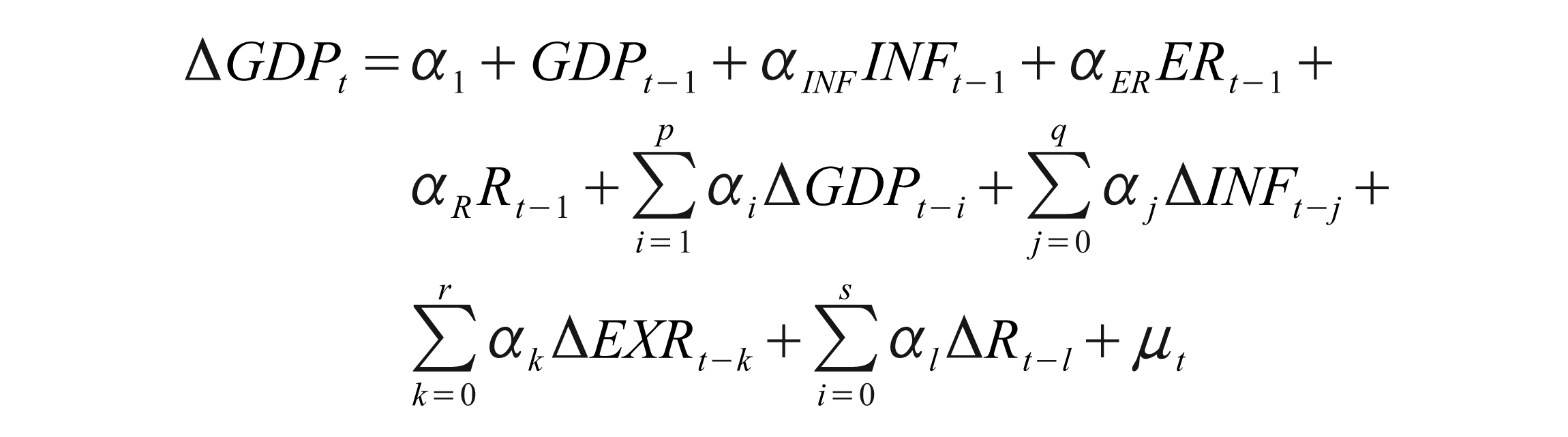
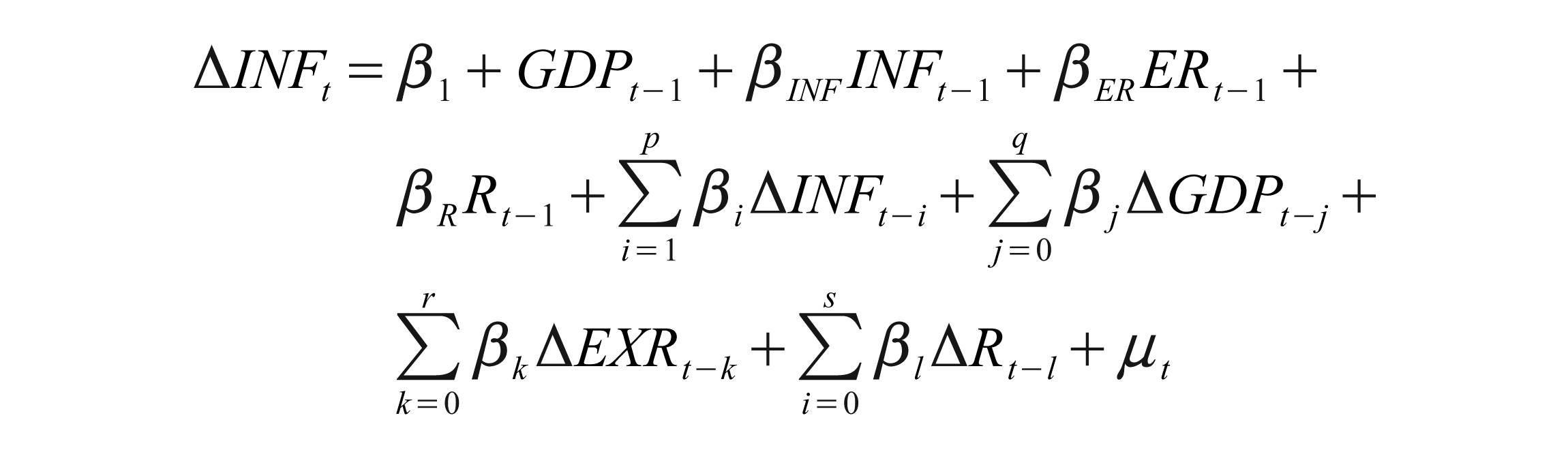
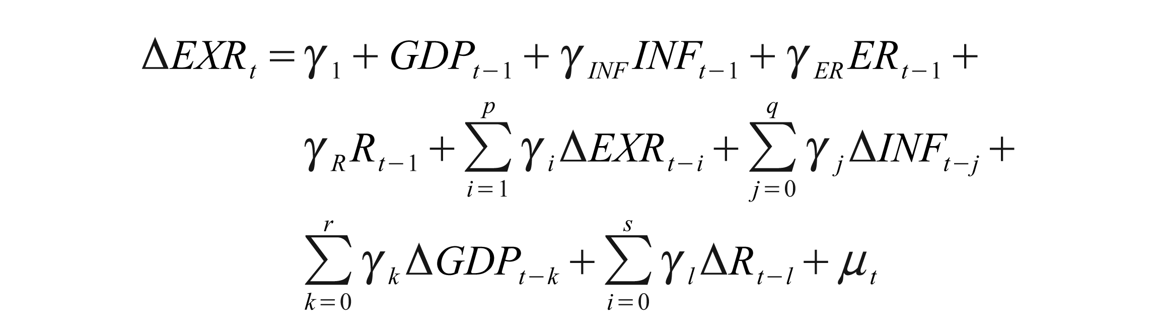
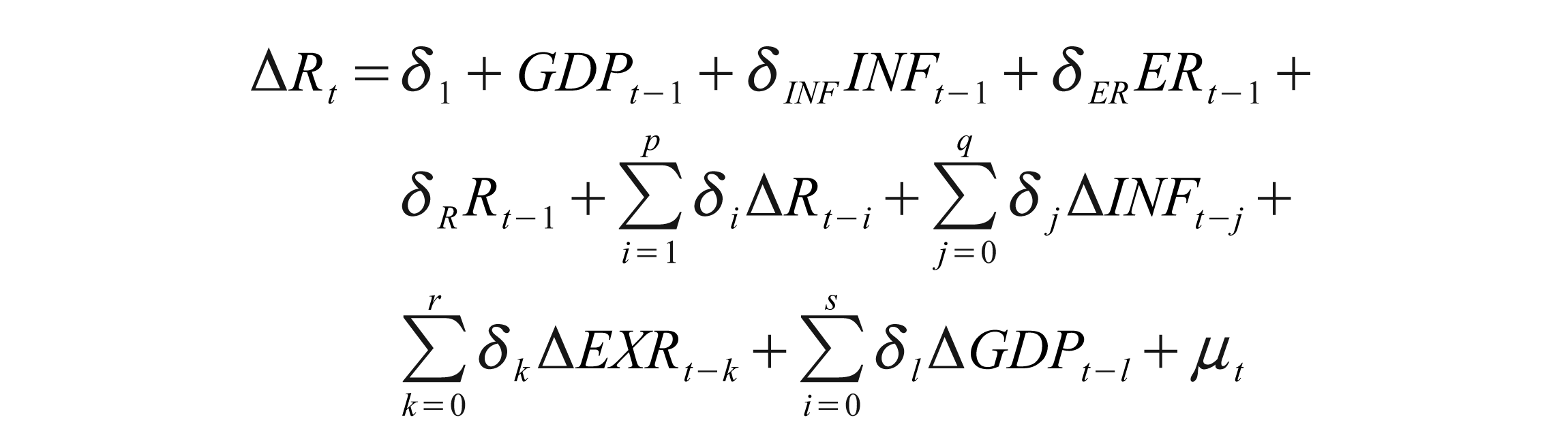
where ∆ is the first difference operator and μ_t are the error terms. The optimal lag structure of the regression is selected by the Akaike information criteriion (AIC) and Schwarz information criterion (SIC). Lags are induced by the noise property in the error term². Pesaran et al. (2001) suggested F-test for joint significance of coefficients of the lagged level of the variables. For example, the null hypothesis of no long-run relationship between the variables in equation (1) is H₀: α_GDP = α_INF = α_EXR = α_R = 0, against the alternative hypothesis of cointegration H₁: α_{GDP ≠} α_{INF ≠} α_{EXR ≠} α_{R ≠} 0.

Two critical bounds are used to test for cointegration, the lower bound is applied if the regressors are I (0) and the upper bound is used for I (1). If the F-statistic exceeds the upper critical value, we conclude in the favour of a long-run relationship; still, if the F-statistic falls below the lower critical values, we can’t reject the null hypothesis of no cointegration. Nevertheless, if the F-statistic lies between the two bounds, the inference would be inconclusive. Once the order of integration for all the series is known to be I (1), the decision is made based on the upper bound. Likewise, if all the series are I (0), then the decision is made based on the lower bound. The robustness of the ARDL model has been checked by using some diagnostic tests. The diagnostic test check serial correlation, functional form, heteroskedasticity and normality of error term.

After investigating the long-run relationship between the variables, we used the Granger causality test to know the causality between the variables. If there is cointegration, an error correction model can be developed as follows:

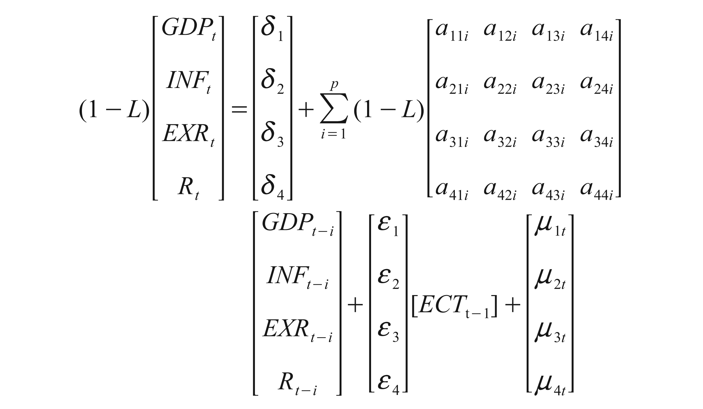
\begin{matrix} \begin{matrix} (1 - L) [\begin{matrix} G D P_{t} \\ I N F_{t} \\ E X R_{t} \\ R_{t} \end{matrix}] = [\begin{matrix} δ_{1} \\ δ_{2} \\ δ_{3} \\ δ_{4} \end{matrix}] \end{matrix} + \sum_{i = 1}^{p} (1 - L) [\begin{matrix} a_{11 i} & a_{12 i} & a_{13 i} & a_{14 i} \\ a_{21 i} & a_{22 i} & a_{23 i} & a_{24 i} \\ a_{31 i} & a_{32 i} & a_{33 i} & a_{34 i} \\ a_{41 i} & a_{42 i} & a_{43 i} & a_{44 i} \end{matrix}] \\ \begin{matrix} [\begin{matrix} G D P_{t - i} \\ I N F_{t - i} \\ E X R_{t - i} \\ R_{t - i} \end{matrix}] \end{matrix} + [\begin{matrix} ε_{1} \\ ε_{2} \\ ε_{3} \\ ε_{4} \end{matrix}] [E C T_{t - 1}] + [\begin{matrix} μ_{1 t} \\ μ_{2 t} \\ μ_{3 t} \\ μ_{4 t} \end{matrix}] \end{matrix}

where 1 – L is the difference operator; ECT_t–1 is the lagged error correction term, which is obtained from the long-run cointegration relationship. The long-run causation is shown by significant t-statistic of the lagged error correction term. The presence of a significant relationship in first differences of the variables provides indication on the direction of short-run causality. The joint χ² statistic for the first difference lagged independent variables is employed to test the direction of short-run causality between the variables. For instance, a₁₂, i ≠ 0, $\forall_{I}$ indicate that Granger causality runs from inflation to economic growth.

Empirical Result

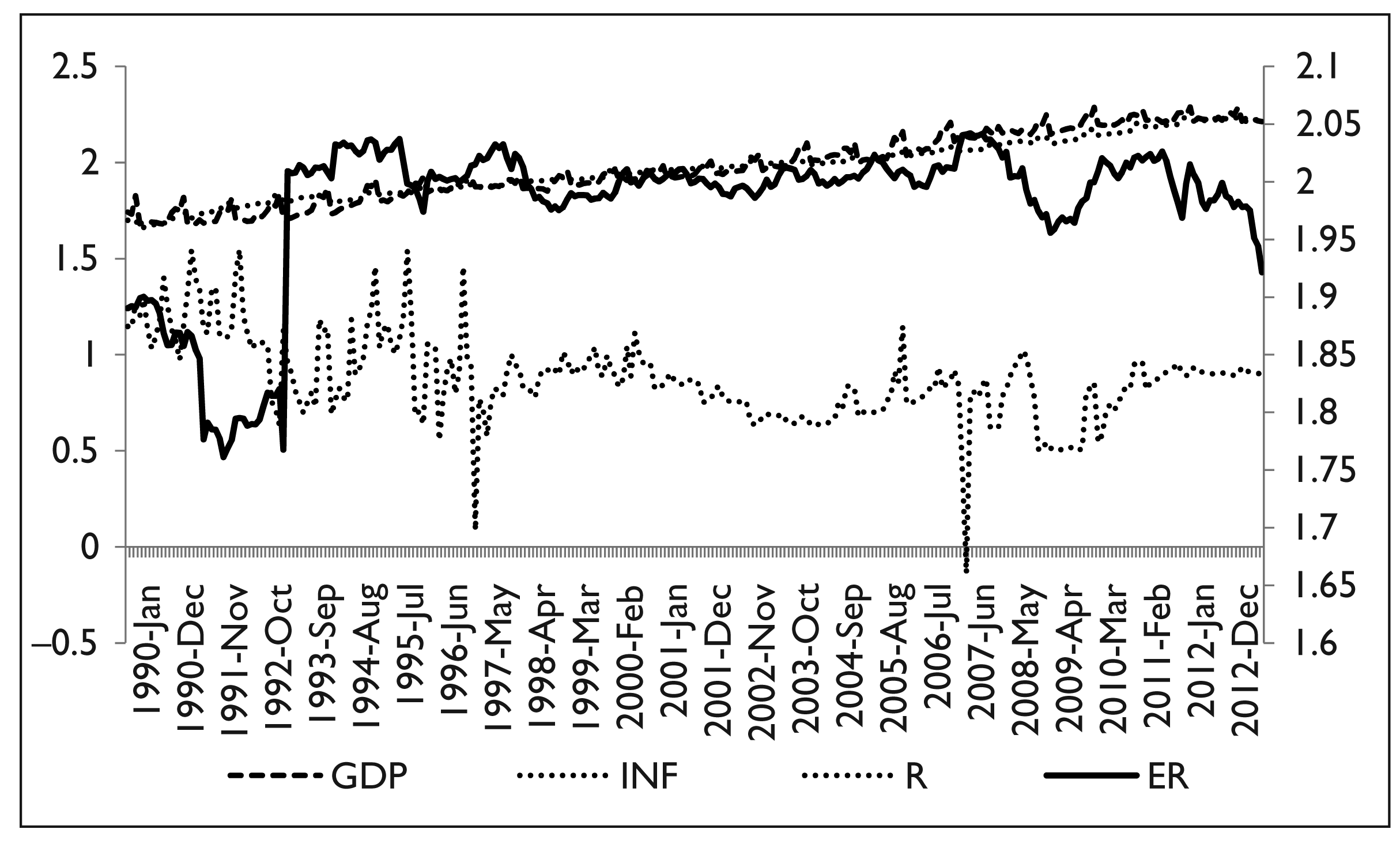
The variables considered in the study for estimating are time series in nature and the frequency of the data collected are monthly in nature. Time series observed at a monthly frequency often exhibit cyclical movements that recur every month. To remove the seasonality among the variables we have employed the US Census Bureau’s X12 seasonal adjustment method by its multiplicative property and removed the seasonality among all the concerned variables. These seasonally adjusted series have been considered for further analysis. To start with, before undertaking any time series econometric analysis of the data, it would be convenient to inspect the broad trends and behaviour of the variables, which may help in interpreting the model results later. For this analysis, time series plots are drawn for all the concerned variables. Figure 1 plots the monthly movement of GDP, inflation, exchange rate and rnterest rates as defined in equation (1). It can be surmised from Figure 1 that there is a close association between the GDP and inflation, and both the series are moving in tandem with each other.

Figure 1.

Source: RBI Handbook of Statistics, 2013.

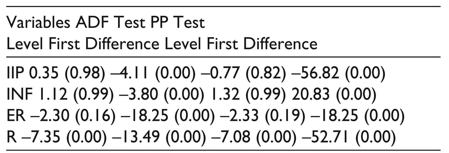
Taking into account the non-stationary nature of most of the time series data, we employ the unit root tests. This is because when the data exhibit unit roots characteristics, the analysis may lead to spurious results and misleading conclusions. Further, the use of cointegration test necessitates the pretest of the presence of unit root in the data. The unit root tests, namely Augmented Dickey-Fuller (ADF) and Phillips-Perron (PP), are conducted to check the stationary property of the data. The results of concerned variables are provided in Table 1. From Table 1, the results show that the null hypothesis of a unit root cannot be rejected for all the concerned variables at their level except interest rates (R). However, the null hypothesis of unit root is rejected for all the variables at their first difference level, and, hence, it can be concluded that they are integrated of order 1 that is I (1) and all the variables at their first difference level are stationary. This result makes the case stronger to examine the long-run association between the variables by employing the ARDL approach which is independent of the order of integration.

Table 1.

Unit Root Test

Variables ADF Test PP Test
Level First Difference Level First Difference
IIP 0.35 (0.98) –4.11 (0.00) –0.77 (0.82) –56.82 (0.00)
INF 1.12 (0.99) –3.80 (0.00) 1.32 (0.99) 20.83 (0.00)
ER –2.30 (0.16) –18.25 (0.00) –2.33 (0.19) –18.25 (0.00)
R –7.35 (0.00) –13.49 (0.00) –7.08 (0.00) –52.71 (0.00)

Source: Authors’ estimation.

Note: The figures in parenthesis show the probability values and the MacKinnon critical values for ADF and PP test of both 1% and 5% level of significance are –3.99 and –3.41, respectively.

Threshold Model Estimation

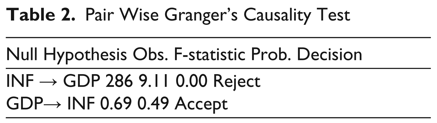
Before we proceed forward to estimate the threshold level of inflation in the Indian context, the short-run causality test is estimated between the economic growth and inflation by employing the Granger’s causality test. The logical rationale behind this test is to identify the endogenous variable between inflation and growth, which will be used in the threshold spline regression model. The pairwise causality test results are reported in Table 2. As per equations (2) and (3), the optimum lag length computed by both the AIC and FPE (Final Prediction Error) criterion is two months. The result reveals that there is a unidirectional causality that exists in between inflation and growth and the causality runs from inflation to growth.

Table 2.

Pair Wise Granger’s Causality Test

Null Hypothesis Obs. F-statistic Prob. Decision
INF → GDP 286 9.11 0.00 Reject
GDP→ INF 0.69 0.49 Accept

Source: Authors’ estimation.

Note: ‘→’ indicates the causality.

The estimation of equation (1) gives a precise value of threshold inflation level and also quantifies the impact of that level of economic growth (Table 3). For this purpose, equation (1) is estimated and the RSS for threshold level of inflation ranging from K₁ to K_n per cent. From Table 3, it can be observed that from the estimated result at k = 4, there is a significant relationship between the dummy of a threshold level of inflation and economic growth. At k = 4, the value of R-square is 0.027. As k starts to increase, R-square decreases and at k = 9, the value of R-square is low, that is, 0.010. At the same time when k = 4, the RSS value is low, that is, 15993.2. As k starts to increase, the value of RSS also increases and it becomes higher when k = 9, that is, 16272.80. Therefore, we conclude that 4 per cent level is the threshold level of inflation, which is obtained by finding that value of k which maximizes the R-square and minimizes the RSS.

Table 3.

Estimation of Threshold Model at K = 3 to 9 (Dependent Variable: GDP Growth Rate)

K	Variable	Coefficient	Std. Error	t-statistic	Prob.	R-squared	RSS
3%	C	–1.494517	4.584729	–0.325977	0.7447	0.023510	16054.21
	INF	–0.001540	0.015088	–0.102049	0.9188
	ER	0.020806	0.042759	0.486600	0.6269
	R	0.003660	0.103959	0.035202	0.9719
	DUMMY	4.778155	1.856262	2.574073	0.0106
4%	C	–1.075803	4.565550	–0.235635	0.8139	0.027219	15993.23
	INF	–0.001962	0.015065	–0.130210	0.8965
	ER	0.017001	0.042577	0.399313	0.6900
	R	0.000895	0.103780	0.008624	0.9931
	DUMMY	5.273764	1.898689	2.777581	0.0058
5%	C	–1.686794	4.597361	–0.366905	0.7140	0.021651	16084.78
	INF	–0.001309	0.015100	–0.086694	0.9310
	ER	0.021667	0.042843	0.505740	0.6134
	R	0.019486	0.104140	0.187114	0.8517
	DUMMY	5.158696	2.091592	2.466397	0.0142
6%	C	–1.805001	4.597468	-0.392608	0.6949	0.023020	16062.26
	INF	–0.002711	0.015124	–0.179259	0.8579
	ER	0.024593	0.042920	0.572986	0.5671
	R	0.017827	0.104035	0.171353	0.8641
	DUMMY	5.748108	2.257607	2.546107	0.0114
7%	C	–2.205981	4.636405	–0.475796	0.6346	0.018907	16129.84
	INF	–0.003350	0.015195	–0.220466	0.8257
	ER	0.029747	0.043420	0.685092	0.4939
	R	0.020066	0.104312	0.192365	0.8476
	DUMMY	6.034324	2.624655	2.299093	0.0222
8%	C	–1.930341	4.667575	–0.413564	0.6795	0.010846	16262.42
	INF	–0.002382	0.015256	–0.156136	0.8760
	ER	0.026607	0.043738	0.608318	0.5435
	R	0.018539	0.104781	0.176929	0.8597
	DUMMY	4.821511	2.798191	1.723081	0.0860
9%	C	–1.962036	4.676689	–0.419535	0.6751	0.010214	16272.80
	INF	0.000302	0.015171	0.019905	0.9841
	ER	0.024332	0.043551	0.558704	0.5768
	R	0.023581	0.105044	0.224487	0.8225
	DUMMY	7.518413	4.501908	1.670051	0.0960

Source: Authors’ estimation.

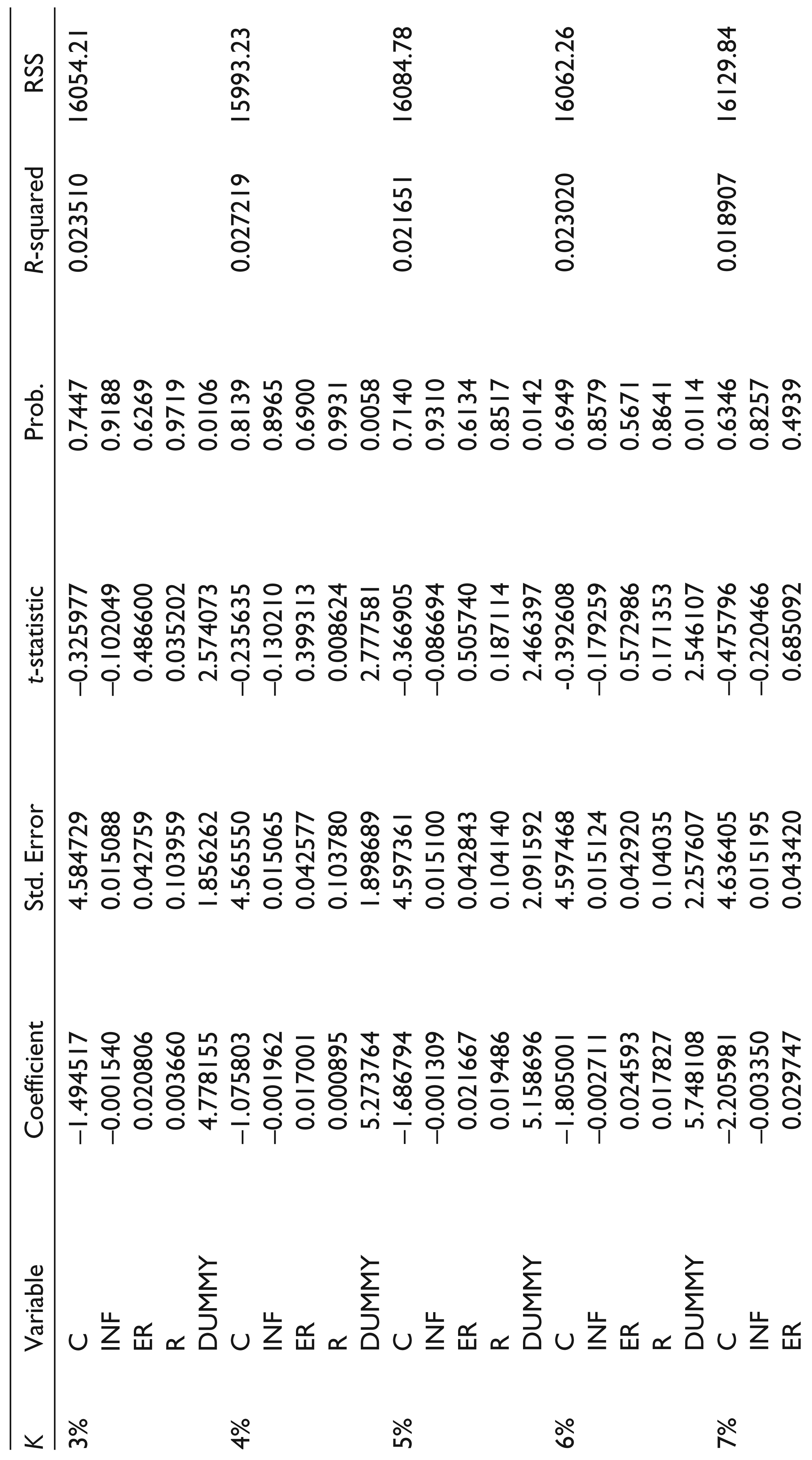
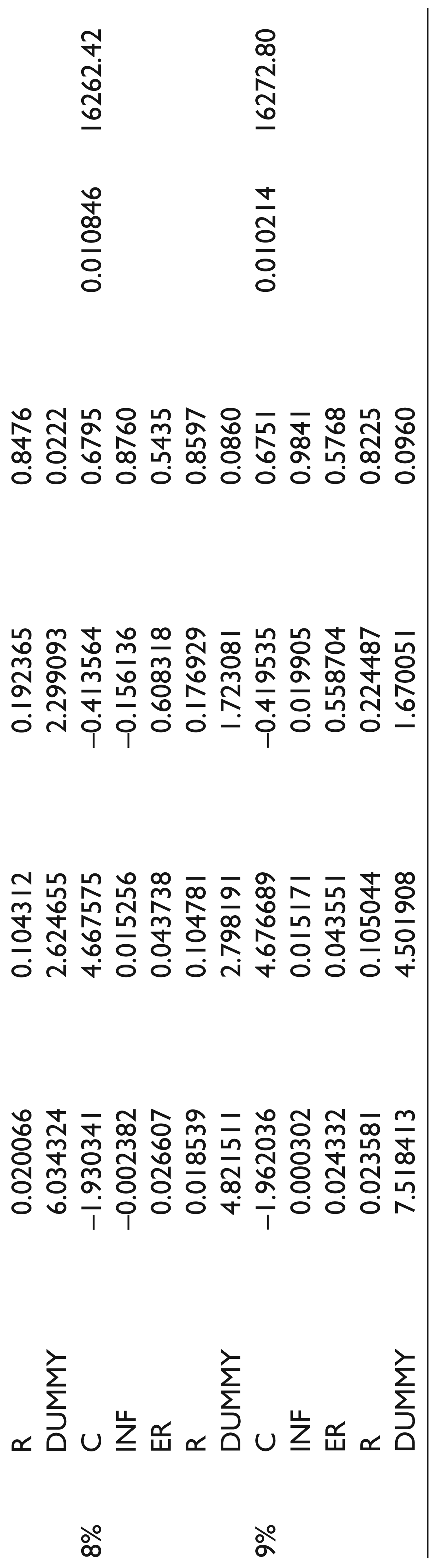
As we know, if there is no inflation an economy may slip into deflation, that is, decrease in prices. Subsequently, decrease in prices leads to less productivity and wage cuts, a threshold level inflation will provide a safer barrier against the negative consequences. Moreover, the threshold inflation level increases the confidence and optimism of investors, leading to an upsurge in the long-run aggregate supply and thus possibly higher rates of economic growth. Therefore, it can be concluded that if the growth in prices does not exceed 4 per cent, inflation will help to keep the economic growth rate stable. In contrast, if the growth rate of prices exceeds 4 per cent, inflation is likely to become harmful, significantly reducing the growth rate of the Indian economy.

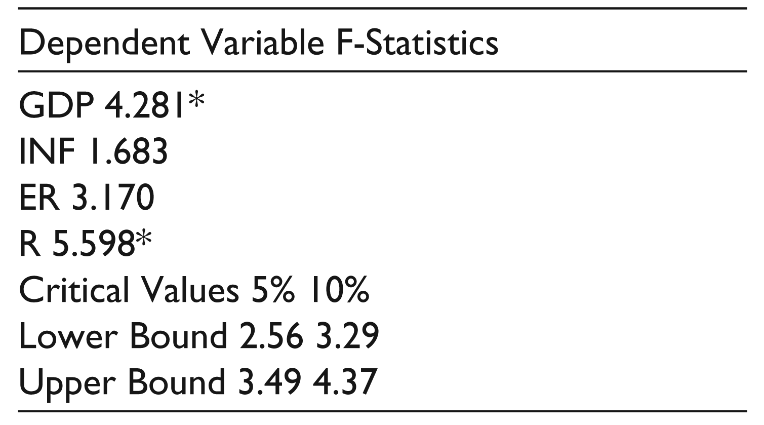
The next step is where equations (4) to (7) are estimated to examine the long-run relationship among the variables. The study used the AIC and Schwarz–Bayesian criteria (SBC) to define the optimal number of lags to be included in the conditional error correction model (ECM), whereas confirming that there was no evidence of serial correlation as emphasized by Pesaran et al. (2001). The lag length that minimizes both the AIC and SBC is two months. The calculated F-statistics for the cointegration test is displayed in Table 4. The critical value is reported together in the same table for both lower and upper bound respectively. The calculated F-statistic (F-statistic = 4.281 and 5.598) of both GDP and the rate of interest (R) is higher than the upper bound critical value at 5 per cent level of significance (3.49). This implies that the null hypothesis of no cointegration cannot be accepted at 5 per cent level and therefore there are two cointegrating vectors existing among the four sets of variables. This result confirms that there is a long-run relationship between economic growth, inflation, exchange rate and rate of interest.

Table 4.

Result of ARDL Cointegration Test

Dependent Variable F-Statistics
GDP 4.281*
INF 1.683
ER 3.170
R 5.598*
Critical Values 5% 10%
Lower Bound 2.56 3.29
Upper Bound 3.49 4.37

Source: Authors’ estimation.

Note: * show the significance at 5% level.

Since there are two cointegrating vectors found among the variables we can estimate the long-run relationship. Table 5 shows that inflation is positively related to GDP and highly significant at the 1 per cent level, whereas the other variables like exchange rate and the rate of interest are not found to be statistically significant. Then the short-run elasticities are computed for the coefficients of the variables at their respective first difference level. The short-run results are reported in the lower panel of Table 5. The short-run result shows that inflation exerts a positive impact on economic growth and statistically significant at the 1 per cent level. However, exchange rate and the rate of interest are insignificant. Therefore, this result reveals that economic growth will increase by 1.13 per cent due to 1 per cent increase in inflation rate.

Table 5.

Long-run and Short-run Analysis

Dependent Variables = GDP
Long-run Results
Variables Coefficients t-statistics
Constant –0.391* –4.691
INF 1.138* 62.294
ER 0.064 1.553
R –0.000 –0.070
Short–run Results
Dependent Variable = DGDP
Variables Coefficients t-statistics
Constant –0.001 –1.056
DINF 1.788* 13.553
DER 0.036 0.412
DR 0.017 1.847
ECT_t–1 –0.226* –6.611
Note: * denote the significance at the 1% level.
Result of VECM Granger Causality
Variables GDP INF ER R ECT_t–1
GDP –28.12* (0.00) 12.85* (0.00) 12.35* (0.00) –0.19* (–4.09)
INF 14.74* (0.00) –18.68* (0.00) 18.58* (0.00) –0.00 (–0.43)
ER 5.52* (0.00) 4.93* (0.00) 4.93* (0.00) 5.51* (0.00) –0.03 (0.02)
R 31.95* (0.00) 46.83(0.00) 46.8 (0.00) –0.95 (1.12)

Source: Authors’ estimation.

Note: * indicates significance at the 5% level. Figure in the parenthesis is the p-value for variables and t-statistics for ECT (Error Correction Term).

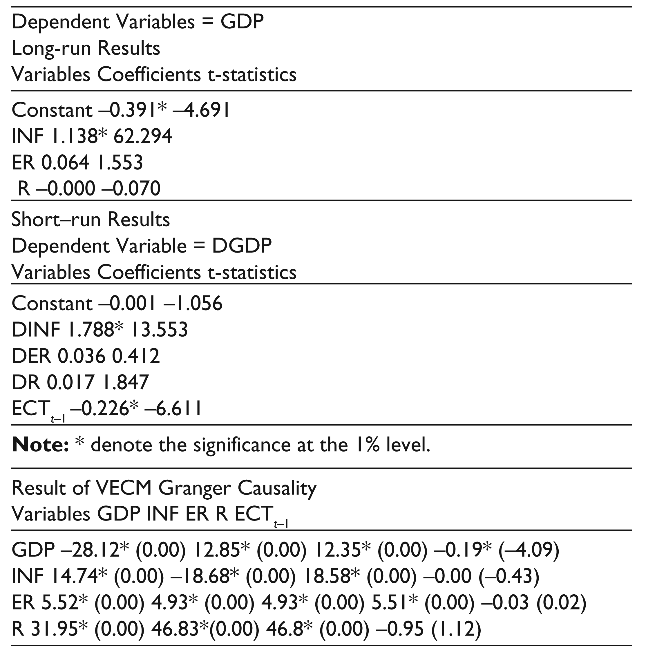
The importance of error correction term shows that change in the response variable is a function of disequilibrium in the cointegration relationship and the changes in other explanatory variables. The coefficient ECT_t–1 implies a speed of adjustment from short run to long run and it is statistically significant. Bannerjee et al. (1998) suggested that significant lagged error term with negative sign is a method to prove that the established long-run relationship is stable. In each period the deviation of economic growth form short-run to long-run is carried out by 22.6 percent. The ARDL model has been shown to be robust against residual autocorrelation model. Therefore, the presence of autocorrelation does not affect the estimates. Hence, the time series constituting both the equations are different orders of integration.

In the previous section, the simple Granger’s causality framework is applied to find out the direction of causality between economic growth and inflation in order to find out the endogenous variable for threshold level estimation. However, the other variables such as interest rate and exchange rate are not considered in the Granger’s causality test to check the direction of causality among the system of variables. The finding on the existence of the long-run equilibrium relationship between the system of variables needs that at least there should be a unidirectional causality between the variables at any direction. Henceforth, the causality test can also be considered as a diagnostic test for cointegration. To examine this possible causal relationship, the study applied VECM causality to detect the direction of causality between the variables for both short run and long run. The empirical results of our study suggest that ECT_t–1 has a negative sign and is statistically significant in the growth equation. This implies that there is a bidirectional caus-ality between economic growth and other varibales in the long run as well as short run.

Concluding Remarks

The major objective of this article is to examine the threshold level of inflation in the framework of growth–inflation relationship. To analyze this, we have applied the spline regression model on the monthly data spanning from January 1990 to December 2013. The empirical results found that there exists a statistically significant structural break in the relationship between inflation and economic growth at 4 per cent. The study suggests that if inflation exceeds beyond the threshold point, that is, 4 per cent, it will negatively affect economic growth.

The ARDL model bound testing cointegration test suggests that there are two cointegration vectors when GDP and the rate of interest are considered as dependent variables. This result confirms that the existence of the long-run equilibrium relationship among economic growth, inflation, exchange rate and rate of interest. From the long-run analysis, the study found that inflation is positively related to economic growth, whereas the other variables are not significant. However, the short-run result shows that inflation exerts a positive impact on economic growth and this is highly statistically significant. The short-run analysis confirms that economic growth will increase by 1.13 per cent due to 1 per cent increase in inflation rate. The error correction result reveals that the deviation of economic growth from short run to long run is carried by 22.6 per cent in each period. The error correction Granger causality test detects that there is a bidirectional relationship among the variables both in the short run as well as in the long run in case of the growth equation.

From the policy implication point of view, the finding that there is a positive relationship between inflation and growth both in the long run and short run suggests that the policy makers should take into account the threshold level inflation in order to escape the jeoparadization effect of inflation on economic growth with caution. It must be emphasized here that the concepts of inflation targeting and inflation threshold are distinct. Inflation targeting is the contrast of money making wherein the central bank declares a target and then steers its policy tools towards achieving that target. Inflation threshold is the point of inflection for the growth and inflation trade-off. Therefore, inflation threshold need not necessarily be the target of monetary policy. Actually, the inflation objective or the target level of inflation for monetary policy should be lower than the threshold inflation considering the existence of significant lags in the transmission mechanism of monetary policy measures and the costs of inflation (Mohanty et al., 2011).

Footnotes

Acknowledgements

The article has benefited from comments by an anonymous reviewer of this journal. The remaining errors are our own.

Notes

Appendix

The summary of the statistical moments of all the variables is presented in Table A1. From this table, it can be seen that the coefficient of skewness, an indicator used in the distribution analysis as a sign of asymmetry, for all the variables is greater than zero. This further suggested that all the variables except exchange rate are positively skewed and most of the values for these variables are concentrated on the left of the mean with extreme values to the right. However, the nominal bilateral exchange rate of the Indian rupee versus the US dollar follows a negatively skewed distribution. The kurtosis coefficient, a measure of the thickness of the tail of the distribution, is quite high in case of exchange rate and the interest rates. A Gaussian (normal) distribution has kurtosis equal to 3 implying that the assumption of Gaussianity cannot be made for the distribution of the concerned variables. Nevertheless, the variables such as IIP (proxy for GDP) and Inflation (INF) follow the platykurtic distribution flatter than a normal distribution with a wider peak. In these cases, the probability for extreme values is less than for a normal distribution and the values have wider spreads around the mean. On the other hand, both exchange rate (EXR) and interest rate (R) follow a leptokurtic distribution, sharper than the normal distribution, with values concentrated around the mean and thicker tails. That means high probability for extreme values. This finding is further strengthened by Jarque–Bera test for normality, which in our case yields very high values—much greater than for a normal distribution, and thus rejects the null hypothesis of normality at any conventional confidence levels for all the variables.

In line with the findings that there is a close association between growth and inflation from Figure 1, the pairwise correlation matrix is constructed in order to find out the co-movement analysis between the variables. The pairwise correlation coefficient along with their corresponding t-statistics is reported in Table A2. From this table, it can be seen that there is a high positive pairwise correlation between GDP and inflation rates. However, there is a low negative pairwise correlation between interest rate and exchange rate, interest rates and GDP, and in between interest rate and inflation. The negative correlation between nominal interest rates and exchange rates may be due to the fact that inflation shocks dominated interest rates and exchange rate movements.

References

Ahmed

, & Mortaza

G. M.

(2005). Inflation and economic growth in Bangladesh: 1981–2005 (Working Paper Series No. WP 0604). Bangladesh: Policy Analysis Unit (PAU), Bangladesh Bank.

Andres

, & Hernando

(1999). Does inflation harm economic growth? Evidence from the OECD. Chicago, IL, US: University of Chicago Press.

Andres

, & Hernando

(1997). Does inflation harm economic growth? Evidence from OECD (Working Paper No. 6062). Cambridge, MA: National Bureau of Economics Research.

Banerjee

, Dolado

J. J.

, & Mestre

(1998). Error correction mechanism test for cointegration in single equation framework. Journal of Time Series Analysis. 19(3), 267–283.

Barro

R. J.

(1995, October). Inflation and economic growth (National Bureau of Economic Research [NBER] Working Paper No. 5326). Cambridge, MA: National Bureau of Economics Research.

Barro

R. J.

(1996). Inflation and growth. Federal Reserve Bank of St. Louis Review, 78(3), 153–169.

Behera

(2014). Inflation and its impact on economic growth: Evidence from six South Asian countries. Journal of Economics and Sustainable Development, 5(7), 145–154.

Behera

, & Mishra

A. K.

(2016). Inflation and economic growth in BRICS: Evidence from ARDL bound testing approach. Asian Journal of Economic Modelling, 4(1), 1–17.

Bhaduri

N. S.

(2007). Revisiting the growth inflation nexus: A wavelet analysis (Working Paper No. 77/2013). Chennai, India: Madras School of Economics.

10.

Bhanumurthy

N. R.

, & Alex

(2008). Threshold level of inflation for India (Institute of Economic Growth Discussion Paper Series No. 124/2008). New Delhi: University Enclave.

11.

Bhatia

R. J.

(1960). Inflation, deflation and economic development. Staff Paper, International Monetary Fund, 8(1), 1011–1014.

12.

Cameron

, Hum

, & Simpson

(1996). Stylized facts and stylized illusions inflation and productivity revisited. Canadian Journal of Economics, 29(1), 152–162.

13.

Caporin

, & Di Maria

(2002). Inflation and growth: Some panel data evidence (GRETA Working Paper No. n.02.09). Venice: GRETA.

14.

De Gregario

(1996). Inflation, growth and central banks (The World Bank Policy Research Working Paper No. 1575). Washington, DC: World Bank.

15.

De Gregario

(1992). Effects of inflation on economic growth: Lession from Latin America. European Economic Review, 36(April), 417–425.

16.

Dorrance

(1963). The effects of inflation on economic development. Staff Papers, International Monetary Fund, 1(10), 1–47.

17.

Erbaykal

, & Okuyan

H. A.

(2008). Does inflation depress economic growth? Evidence from Turkey. International Research Journal of Finance and Economics, 17, 1450–2885.

18.

Faria

J. R.

, & Carneiro

F. G.

(2001). Does high inflation affect growth in the long and short run. Journal of Applied Economics, 4(1), 89–105.

19.

Feldstein

(1982). Inflation tax rules and investment: Some econometric evidence. Econometrica, 50, 825–862.

20.

Fischer

(1993). Inflation and growth (NEBR Working Paper No. 1235), pp. 267–278. Cambridge, MA: NEBR.

21.

Friedman

(1956). Quantity theory of money: A restatement. In Frideman

(Ed.), Studies in the quantity theory of money (pp. 3–21). Chicago, IL: University of Chicago Press.

22.

Ghosh

, & Phillips

(1998a). Warning, inflation may be harmful to your growth. IMF Staff Paper, International Monetary Fund, 45(4), 672–710.

23.

Ghosh

, & Phillips

(1998b). Inflation, disinflation and growth (IMP Working Paper No. WP/98/08). Washington, DC: IMF.

24.

Gillman

, Harris

, & Maytas

(2002). Inflation and growth some evidence. Paper presented at the 10th International Conference on Panel Data, Berlin.

25.

Granger

C. W. J.

(1969). Investigating causal relations by econometric model and cross-spectral methods. Econometrica, 37(3), 424–438.

26.

Gylfason

(1998). Output gains from economic stabilization. Journal of Development Economics, 56(1), 81–96.

27.

Gylfason

, & Herbertsson

T. T.

(2001). Does inflation matter for growth? Japan and the World Economy, 13(4), 405–428.

28.

Hussain

(2005). Inflation and growth: Estimation of threshold point for Pakistan. Pakistan Business Review, 7(3), 1–15.

29.

Judson

, & Orphanides

(1996). Inflation volatility and growth (Finance and Economics Discussion Series No. 96/19). Washington, DC: Board of Governor of the Federal Reserve System.

30.

Kannan

, & Joshi

(1998). Growth-inflation tradeoff: Empirical estimation of threshold rate of inflation for India. Economic and Political Weekly, 33(42–43), 17–30.

31.

Khan

M. S.

, & Senhadji

A. S.

(2001). Threshold effects in the relationship between inflation and growth. IMF Staff Papers, 48(1), 1–21.

32.

Lee

C. C.

, & Wong

S. Y.

(2005). Inflationary threshold effects in the relationship between financial development and economic growth: Evidence from Taiwan and Japan. Journal of Economic Development, 30(1), 4969.

33.

Lucas

(1973). Some international evidence on output and inflation tradeoff. American Economic Review, 63(3), 326–334.

34.

Malla

(1997). Inflation and economic growth: Evidence from a growth equation. Manao, Honolulu, HI: Department of Economics, University of Hawaia.

35.

Mallik

, & Chowdhury

(2001). Inflation and economic growth: Evidence from South Asian countries. Asian Pacific Development Journal, 8(1), 123–135.

36.

Mohanty

, Chakraborty

A. B.

, Das

, & Jogn

(2011). Inflation threshold in India: An empirical investigation (Reserve Bank of India Working Paper Series No. 18). India: RBI.

37.

Motley

(1998). Growth and inflation: A cross country study. Federal Reserve Bank of Son Francisco, Economics Review, 98(1), 15–28.

38.

Mubarik

Y. A.

(2005). Inflation and growth: An estimate of the threshold level of inflation in Pakistan. State Bank of Pakistan Research Bulletin, 1(1), 35–44.

39.

Munir

, Mansur

, & Furuoka

(2009). Inflation and economic growth in Malaysia: A threshold regression approach. ASEAN Economic Bulletin, 26(2), 180–193.

40.

Naqvi

S. N. H.

, & Khan

A. H.

(1989). Inflation and growth: An analysis of recent trends in Pakistan. Islambad: Pakistan Institute of Development Economics.

41.

Pattanaik

, & Nadhanael

G. V.

(2011). Why persistent high inflation impedes growth? An empirical assessment of threshold level of inflation for India. Department of Economic and Policy Research, Reserve Bank of India, 6(September), 204–220.

42.

Paul

, Kearney

, & Chowdhury

(1997). Inflation and economic growth: A multi country empirical analysis. Applied Economics, 29(10), 1387–1301.

43.

Pesaran

, Shin

, & Smith

(2001). Bound testing approach to the analysis level relationship. Journal of Applied Econometrics, 16(3), 289–326.

44.

Rangarajan

(1998). Development, inflation and monetary policy. In Ahluwalia

I. S.

& Little

I. M. D.

(Eds), India’s economic reforms and development (pp. 48–72). New Delhi: Oxford University Press.

45.

RBI. (1985). Report of the committee to review the working of monetary system. Mumbai: Reserve Bank of India.

46.

Rousseau

P.L.

, & Wachtel

(2002). Inflation threshold and the finance-growth nexus. Journal of International Money and Finance, 21(6), 777–793.

47.

Saeed

A. A. J.

(2007). Inflation and economic growth in Kuwait 1985–2005: Evidence from coinetgration and error correction model. Journal of Applied Econometrics and International Development, 7(1), 143–155.

48.

Samantaraya

, & Prasad

(2001). Growth and inflation in India: Detecting the threshold level. Asian Economic Review, 43(3), 414–420.

49.

Sarel

(1996). Non-linear effects of inflation on economic growth (IMF Working Paper No. WP/95/96). Washington, DC: IMF.

50.

Shi

(1999). Search, inflation and capital accumulation. Journal of Monetary Economics, 44(1), 81–103.

51.

Shrestha

, & Chowdhury

M. K.

(2007). Testing financial liberalization hypothesis with ARDL modelling approach. Applied Financial Economics, 17(18), 1529–1540.

52.

Sidrauski

(1967). Rational choice and patterns of growth in a monetary economy. American Economic Review, 57(2), 534–544.

53.

Sims

C. A.

(1972). Money, income and causality. The American Economic Review, 62(4), 540–552.

54.

Singh

, & Kalirajan

K. P.

(2003). The inflation-growth nexus in India: An empirical analysis. Journal of Policy Modeling, 25(4), 377–396.

55.

Singh

(2010). Searching threshold inflation for India. Economics Bulletin, 30(4), 3209–3220.

56.

Stanners

(1993). Is low inflation is an important condition for high growth. Cambridge Journal of Economics, 17(1), 79–107.

57.

Stockman

A. C.

(1981). Anticipated inflation and the capital stock in a cash advance economy. Journal of Monetary Economics, 8(3), 387–393.

58.

Sweidan

O. D.

(2004). Does inflation harm economic growth in Jordan? An econometric analysis for the panel 1970–2000. International Journal of Applied Econometrics and Quantitative Studies, 1(2), 41–66.

59.

Tobin

(1965). Money and economic growth. Econometrica, 33(4), 671–684.

60.

Vasudevan

A. B.

, Bhoi

B. K.

, & Dhal

S. C.

(1998). Inflation rate and optimal growth—Is there a gateway to ‘nirvana’? In Vasudevan

(Ed.), Fifty years of development economics: Essays in honor of prof. Brahmannda (pp. 50–67). Mumbai: Himalya Publishing House.