Corporate Debt,Rentiers’ Portfolio Dynamics,Instability and Growth: A Neo-Kaleckian Perspective

Abstract

Considering a stock-flow consistent neo-Kaleckian macromodel of the post-COVID-19 US economy, along with firms’ debt dynamics, in the long run, we incorporate portfolio dynamics of rentiers and investigate the possibility dynamic (in)stability of the economy. Both the debt-led and the debt-burdened demand and growth regimes are possible. We find share buybacks, under certain conditions, not only may lead to the deterioration of the equilibrium rate of capital accumulation in the long-run but may also potentially destabilize the entire economy. A strictly regulated financial market is desirable, as otherwise, the economy may lose its stability and produces the limit cycles. A new paradox in neo-Kaleckian tradition, the paradox of share buybacks is also uncovered in this article.

JEL Classification: C62, E12, E32, E44, O41

Keywords

Capital accumulation Kaleckian model stock-flow consistency instability limit cycle

Introduction

This article develops a macromodel in investigating the post-COVID-19 firms’ debt dynamics and rentiers’ portfolio dynamics as coupled dynamics of the US economy in a neo-Kaleckian model of capital accumulation and output growth. One innovative feature of the model is that firms can perform share repurchases or buybacks and while doing so can have an impact on the long-run equilibrium rates of capacity utilization and output growth and on the stability properties of the several long-run equilibrium configurations. In a nutshell, the purpose of this article is to present a neo-Kaleckian stock-flow consistent macroeconomic model of the post-COVID-19 US economy to explain (a) how firms make their decisions related to financial and real sectors, (b) how the rentiers make their portfolio decisions and (c) how the interaction between financial and real sectors leads to (in)stability in the economy. A new paradox, the paradox of share buybacks, is uncovered in this article. A rise in share buybacks, and hence a higher (respectively lower) fraction of investment being financed by debt (respectively issuance of equities), may lead to a higher instead of lower ratio of equity to debt in the long-run equilibrium.

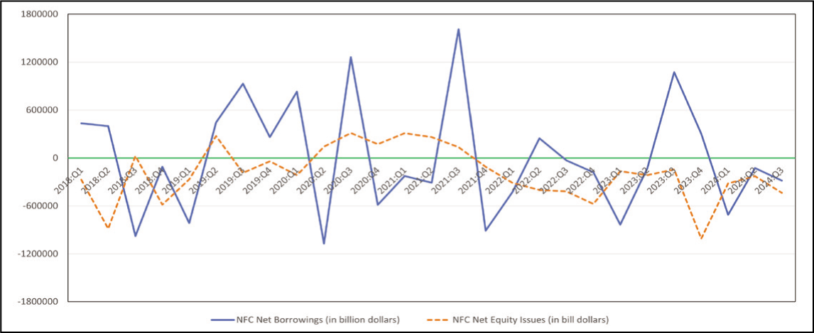
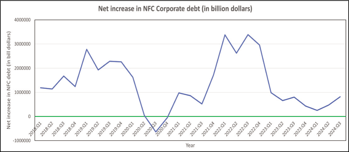
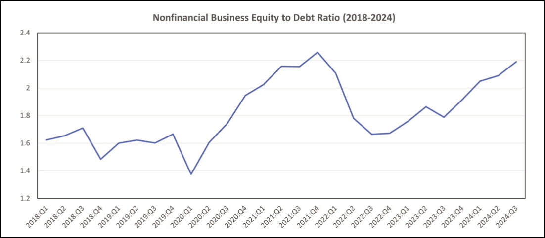
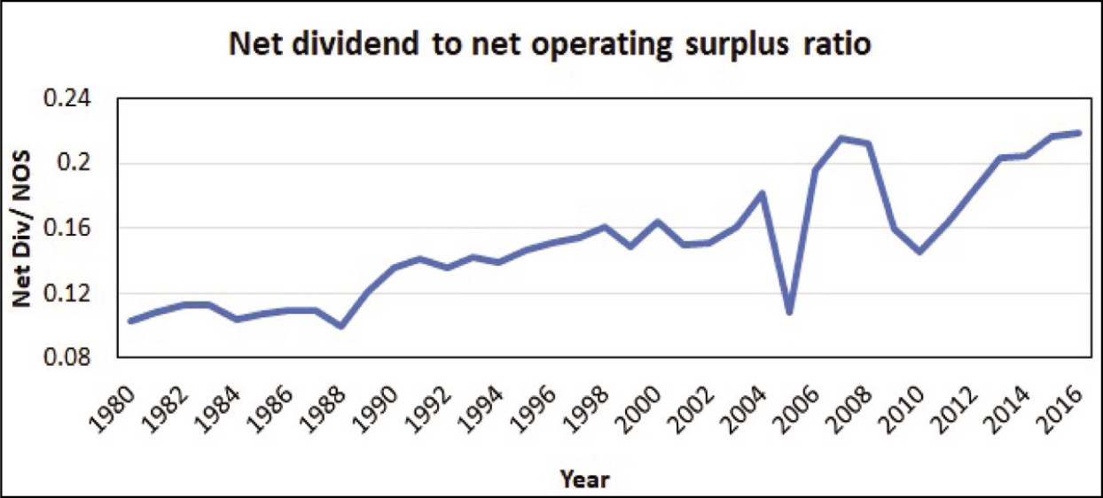
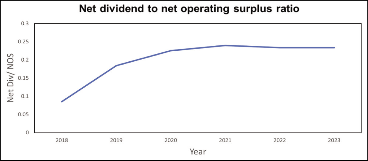
The COVID-19 pandemic has once again forced us to realize the importance of maintaining financial and real sector stability in particular in the context of the US economy. We observe a perpetual rise in corporate debt and share buybacks in the US economy in the post-COVID-19 phase. Domestics nonfinancial sectors debt liabilities have also been a striking feature. Starting from $72,052,657 billion in the first quarter of 2018, it increases to $102,903,790 billion in the third quarter of 2024.¹ Figure 1 exhibits the new equity issuance (in billion dollars) and new credit market borrowings of non-financial corporations (in billion dollars) of the US economy in the post-COVID-19 period. Note that similar to the post-1980s till the US financial crisis (2007), in the post-COVID-19 period also there is a negative trend in the issuance of new equities. In other words, there is a share buyback happening in the post-COVID-19 period. At the same time, there is a continuous rise in the non-financial business debt of the corporate sectors (see Figure 2). We observed a similar trend in the 1980–2007 period, where instead of financing investment projects, a significant portion of the corporate borrowing was spent on equity buybacks. We also observe a dramatic fluctuation in the corporate equity-to-debt ratio (see Figure 3). Therefore, a macroeconomic analysis is required that addresses all the above issues. However, as the US economy is suffering from a demand deficiency, a supply-side macromodel will not help us investigate the problems. Consequently, in this article, we construct a neo-Kaleckian macromodel of capital accumulation and output growth that tries to explain how real and financial sectors-related decisions are taken by the firms, how the rentiers make their portfolio decisions, and how the interaction between the real and financial sectors may cause instability in the economy. We also investigate the impacts of a rise in share buybacks and interest rates in (de)stabilizing the economy. We advocate for a policy of a more regulated financial market and stringent rules/regulations on share buybacks to stabilize the economy.

Figure 1.

Source: Flow of Funds, Table L.100, Board of Governors of the Federal Reserve, 12 December 2024.

Figure 2.

Source: Flow of Funds, Table L.100, Board of Governors of the Federal Reserve, 12 December 2024; author’s calculations.

Figure 3.

Source: Flow of Funds, Table L.100, Board of Governors of the Federal Reserve, 12 Decem.ber 2024; author’s calculations.

Although neo-Kaleckian theory of growth and distribution started with the contribution of Rowthorn (1981), Dutt (1984), Taylor (1985), Amadeo (1986), Blecker (1989), Bhaduri and Marglin (1990) and Marglin and Bhaduri (1990), financial variables have been introduced much later in this tradition. While Hein (2006, 2007, 2008a, 2008b, 2012b), Lima and Meirelles (2007), Charles (2008a, 200b) and Parui (2022) introduce firms’ debt dynamics in the Kaleckian growth model and investigate the financial fragility and instability in the economy, Dutt (2006), Hein (2012a, 2012b), Kim (2012), Kim et al. (2014), Kapeller and Schütz (2015), Setterfield and Kim (2016), Setterfield et al. (2016) and Parui (2023) are among others who capture the workers’ debt dynamics in the Kaleckian tradition.

In a neo-Kaleckian model of growth and distribution with excess capacity, by endogenizing the retention rate and the level of debt, Charles (2008a) investigates the conditions for multiple equilibria and the possibility of instability. However, some problems with his model can be observed. First, Charles (2008a) assumes a positive relationship between the retention ratio and the debt level. According to him, in the case of a higher level of debt, ‘to preserve their financial autonomy and their ability to meet financial commitments’, firms reduce dividend payment and increase the retention ratio. However, in the era of financialization, precisely the opposite of that happens. A higher level of debt results in a higher level of risk and financial fragility. Consequently, shareholders would demand higher dividends for compensating the high level of risk. Dividend can also be perceived (by shareholders) as a signal for profitability, financial strength and stability of firms (Baker & Wurgler, 2002). Therefore, when there is a higher level of risk caused by a higher level of debt, firms would prefer to provide a higher level of dividend as a signal of its financial stability to the shareholders. Dallery and Treeck (2011) also validate this. Second, Charles (2008a) assumes debt–capital ratio as the only determinant of targeted retention ratio. Along with the debt–capital ratio, however, expected future profit rate and expected growth rate are also key determinants of firms’ targeted dividend capital ratio. However, this is missing in his analysis.

Charles (2008b) develops a simple post-Keynesian macromodel and shows the instability in the economy because of a change in interest rate. Charles endogenizes the interest rate that fluctuates due to the change in debt–capital ratio or due to change in the exogenous interest rate of the riskless assets. According to him, the higher the debt–capital ratio, the higher are the borrower’s risk and the rate of interest (of risky assets). While growing interest rate can destabilize the economy, an easy monetary policy can prevent the economy from collapsing.

Taylor and Rada (2003) construct a post-Keynesian macromodel related to cycles of business debt and equity. Over the past 50–100 years, according to them, six secular debt–equity cycles occur in data for the USA, UK and Japan. A clockwise pattern is observable for the USA and the UK while in case of Japan, a counterclockwise pattern is followed. The clockwise pattern arises for a ‘debt-led’ capital accumulation rate and an ‘equity accelerated’² debt–capital ratio, whereas a ‘debt-burdened’ capital accumulation rate and an ‘equity-decelerated’ debt–capital ratio lead to the occurrence of counterclockwise cycles.

Ryoo (2010), in a stock-flow consistent macromodel, shows the financial fragility that evolves endogenously through the interaction between real and financial sectors due to firms’ and households’ financial practices. Ryoo provides two distinct cycles: long waves and short cycles. An interaction between firms’ and households’ financial decisions generates long waves, whereas an interaction between effective demand and labour market dynamics produces short cycles. In his model, firms decide how much to accumulate and how to finance it; households take the consumption and portfolio decisions, and banks receive deposits and create loans. There are only two types of financial assets: equity and bank deposits. He assumes that there is a constant growth in the available labour force, and the long-run growth is constrained by it.

The mechanism of long waves depends on two subsystems: (a) changes in firms’ liability structure (i.e. the debtcapital ratio) and (b) changes in households’ portfolio composition (i.e. the equitydeposit ratio). In the long run, a change in firms’ debtcapital ratio depends on the ratio of the trend rate of profit to the interest payment obligation. If the level of profit is sufficiently high compared to interest payment obligations, firms are eager to take more debt while banks are willing to provide the required debt as higher profit level compared to an interest payment of firms is perceived by banks as having a lower probability of default. Banks play a passive role, and the availability of credit is independent of the financial position of banks. Households’ equity-to-deposit ratio (or, in other words, households’ portfolio decision) depends on households’ optimism about stock markets, which in turn depends on the difference between the rates of return on stocks and deposits. ‘Capital gains from holding stocks are not assumed away and enter the definition of the rate of return on equity’. During good years, households tend to hold a more significant proportion of financial assets in the form of riskier assets, that is, on equity. In this model, in the long run, these above-mentioned two stable subsystems, when interacting with each other, can produce instability and cycles in the whole system.

For the short cycles, output growth is determined by the labour market conditions and profit signals in the goods market. Higher profitability instigates firms to expand output, whereas the tightened labour market provides negative incentives to the firms for expanding production. On the other hand, growth in the employment rate is determined by the difference between the output growth and the growth in the available labour force, which grows exponentially at a constant rate. Then Ryoo (2010) integrates long waves with short cycles and provides some simulation results.

However, Ryoo (2010) assumes equity finance as a pure residual of firms’ financing constraint as it serves as a buffer to fill the gap between the funds needed for the investment plans and the funds available from retained earnings and bank loans. However, it is very unlikely that for a sufficiently long period, funds needed for the investment plans of firms are lower than the available fund from retained earnings and borrowings so that they can adjust the excess funds by repurchasing stocks. We elabourately discuss it later in the third section.

A few essential features of our model are: first, the model is stock-flow consistent. Second, although the economy is always in a wage-led demand regime, both the debt-led and the debt-burdened demand and growth regimes are possible. Third, the interaction between the dynamics of debt–capital ratio and the equity-debt ratio allows the existence of multiple equilibria and opens the possibility of instability in the economy. Fourth, share buybacks, under certain conditions, not only may lead to the deterioration of the equilibrium rate of capital accumulation in the long-run but may also potentially destabilize the entire economy.

The outline of the rest of the article is as follows. The second section sets up the model and talks about the short-run analysis and the short-run comparative statics. The third section discusses the long-run analysis where we endogenize the debt–capital ratio and the equity-debt ratio. The fourth section discusses several possible cases which may arise because of the interaction between the debt–capital ratio and the equity-debt ratio dynamics. This is followed by the fifth section which talks about the comparative statics. The sixth section offers some concluding remarks.

The Model

We assume a simple one-sector, closed-economy, neo-Kaleckian growth model in which the economy consists of workers, rentiers and firms. Neither government intervention nor technical progress is there. Income is distributed between wages and profits as

pY = wL + rpK = W + R,

(1)

where p is the price level, Y is the real income, w is the nominal wage rate, L is the total amount of labour employment, K is the existing real capital stock, $r = \frac{R}{{}_{P}K}$ is the real rate of profit, W is the nominal wage income and R is the nominal profit income. As this is a one-good model, for the sake of simplicity, we assume the price of the commodity as unity, that is p = 1. Consequently, Y now is the real as well as the nominal output level and K is the existing real as well as the nominal capital stock. Therefore, Equation (1) becomes

Y = W + R

(2)

where Y is nominal income, W is nominal wage income and R is nominal profit income. We assume excess supply of labour and under-utilization of capacity in the economy. For simplicity, we assume away depreciation of capital stock. The production function is of Leontief type, that is,

Y = \min {a L, b K} = a L; b = \frac{Y^{F}}{K} > \frac{Y}{K},

(3)

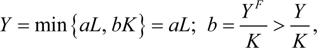
where Y^F is the potential output level. So the actual output is below the potential output level.

We assume two types of households: workers and rentiers. Workers do not hold any asset and earn from only one source of income, the wage income (W). We assume workers consume whatever they earn, that is,

CW = W = [(1 - π) u] K,

(4)

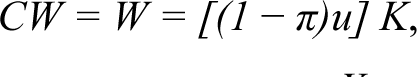
where C_W is consumption of workers, $u = \frac{Y}{K}$ is the degree of capacity utilization,³ $π = \frac{R}{Y}$ is the share of profit (which is fixed in the short-run as well as in the long run)⁴ $r = \frac{R}{Y}$ and is the profit rate. So, r = πu. Note that the wage income is $W = Y - R = Y (1 - \frac{R}{K}) = Y (1 - π) = (1 - π) \frac{Y}{K} K = (1 - π) u K .$ Consequently, the profit income is R = πuK.

Rentiers hold two types of assets: (a) loans to the firms (D) and (b) equities issued by firms (P_eE). Equities are considered to be a more risky asset compared to bank deposits (or loans given to the firms). Rentiers earn their income from two sources: (a) interest income on the funds they lend to the firms (iD) and (b) from a fraction (1 − s_f) of profit (net of interest payment, i.e., R − iD) given to them as distributed profit or dividend by the firms.⁵ Rentiers’ consumption level (CR) depends on their total income (i.e. {(1 − s_f)(R − iD) + iD}) and total wealth (i.e. p_eE + D) as follows:

C_{R} - c_{r} [(1 = s_{f}) (R - i D) + i D) + c_{q} (P_{e} E + D),

(5)

\Rightarrow \frac{C_{R}}{K} = c_{r} [(1 - s_{f}) (π u - i d) + i d] + (1 + λ) c_{q} d

(6)

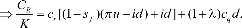
where c_r is the consumption propensity of rentiers out of current income and c_q is the consumption propensity out of wealth,⁶ i is the interest rate on both deposit and loan, D is the total debt of firms to the rentiers, d is the debt-to-capital ratio, $λ = \frac{P_{c} E}{D}$ is the nominal market value of equity-to-debt ratio and s_f is the retention rate of firms.

We assume that the borrowing of firms has to be backed by full collateral. Every unit rise in firms’ borrowing (or a rise in debt) has to be backed by issuing an equal nominal market value of equity. We assume the price of equity (P_e) is fixed to unity in the short-run. Therefore, in the short-run, if firms want to borrow $100, firms have to issue 100 units of equities. In other words, for every unit rise in debt (D), the equity (E) also has to be increased by the same amount. Consequently, for a change in D, E moves in the same direction by same amount in the short-run. One can think of rentiers and firms having naive expectation about the price of equity. However, rentiers and firms know that the price of equity may change in the long run. Therefore, if P_e rises in the long run, rentiers gain and firms lose whereas, for a fall in P_e the reverse happens.⁷

Following the neo-Kaleckian literature, we assume a fraction of profit (or profit net of interest payment) is given as a dividend to the rentiers (see Charles, 2008a, 2008b, for example). Following Charles (2008a, 2008b), we assume the investment demand of firms depends positively on the available internal funds as follows:

I = [α_{0} + α_{1} s_{f} (π u - i d)] K

(7)

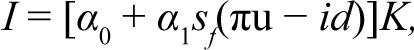
where α₀ represents the state of animal spirits and α₁ is the coefficient measuring the responsiveness of investment–capital ratio to a change in available internal funds. In order to make the model tractable, we assume a very simple investment function (I) that depends only on the state of animal spirits (α₀) and on available internal funds. Our primary purpose in this article is to see the short-run impact of debt and the equity–debt ratio on aggregate demand, income distribution and economic growth and then to investigate the long-run dynamics between debt–capital and equity-debt ratio. Therefore, we concentrate on the role of internal funding on investment decisions and ignore the influence of capacity utilization. However, although Equation (7) does not feature a separate (positive) influence of capacity utilization to it (the standard accelerator effect), it features capacity utilization positively impacting on internal funding (as a proportion of the capital stock). Consequently, ceteris paribus, a rise in the capacity utilization rate leads to a rise in the investment demand. This kind of investment function can be found in Charles (2005, 2008a, 2008b), and the empirical evidence can be found in Ndikumana (1999).

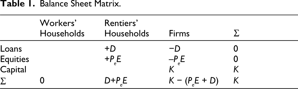
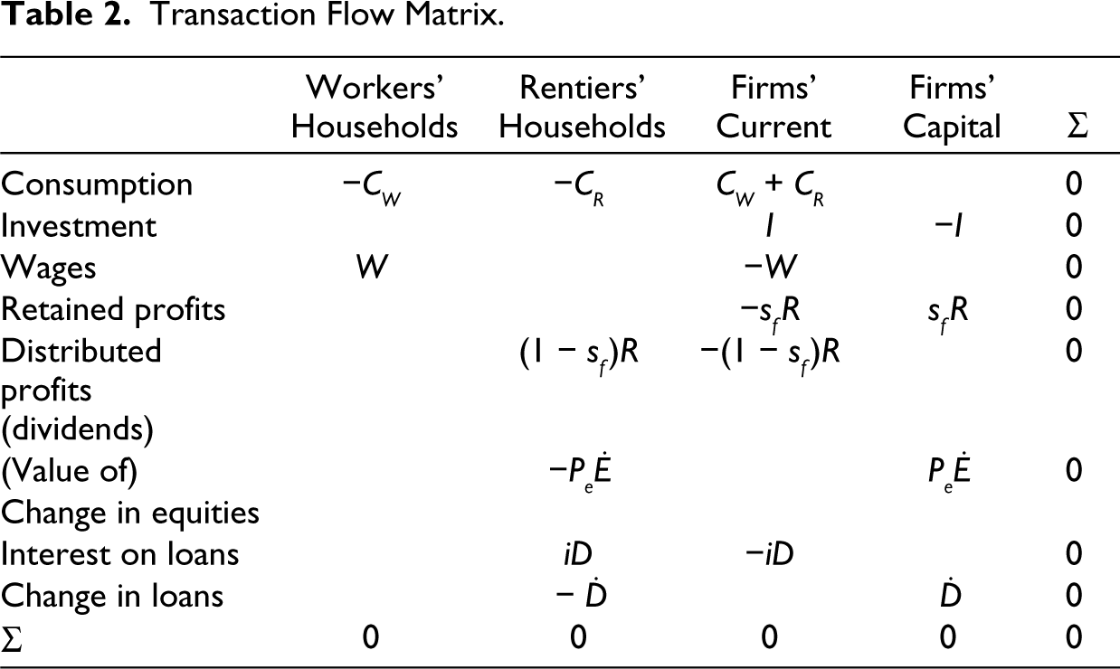
The basic structure of the model is summarized by the balance sheet matrix in Table 1. and the transaction flow matrix in Table 2.

Table 1.

Balance Sheet Matrix.

	Workers’ Households	Rentiers’ Households	Firms	Σ
Loans Equities Capital		+D +P_eE	−D –P_eE K	0 0 K
Σ	0	D+P_eE	K − (P_eE + D)	K

Table 2.

Transaction Flow Matrix.

	Workers’ Households	Rentiers’ Households	Firms’ Current	Firms’ Capital	Σ
Consumption	−C_W	−C_R	C_W + C_R		0
Investment			I	−I	0
Wages	W		−W		0
Retained profits			−s_fR	s_fR	0
Distributed profits (dividends)		(1 − s_f)R	−(1 − s_f)R		0
(Value of)		−P_eE˙		P_eE˙	0
Change in equities
Interest on loans		iD	−iD		0
Change in loans		− D˙		D˙	0
Σ	0	0	0	0	0

Short-run Equilibrium

In the short-run, the goods market is cleared through changes in the level of output and capacity utilization. In equilibrium, nominal income must be equal to aggregate demand, that is,

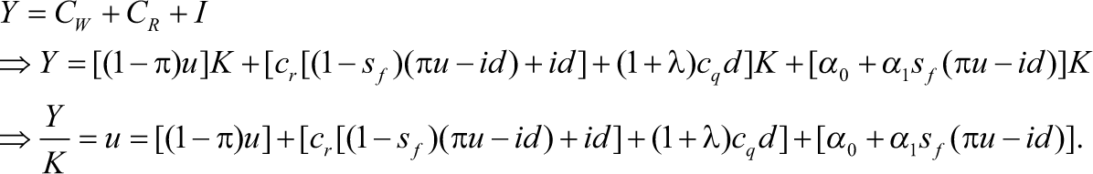
\begin{array}{l} Y = C_{W} + C_{R} + I \\ \Rightarrow Y = [(1 - π) u] K + [c_{r} [(1 - s_{f}) (π u - i d) + i d] + (1 + λ) c_{q} d] K + [α_{0} + α_{1} s_{f} (π u - i d)] K \\ \Rightarrow \frac{Y}{K} = u = [(1 - π) u] + [c_{r} [(1 - s_{f}) (π u - i d) + i d] + (1 + λ) c_{q} d] + [α_{0} + α_{1} s_{f} (π u - i d)] . \end{array}

After some manipulation, it yields the equilibrium degree of capacity utilization as

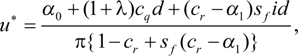
u^{*} = \frac{α_{0} + (1 + λ) c_{q} d + (c_{r} - α_{1}) s_{f} i d}{π {1 - c_{r} + s_{f} (c_{r} - α_{1})}},

(8)

where u* is the equilibrium degree of capacity utilization. We assume the Keynesian stability condition holds, that is, the induced increase in saving as u rises $(i . e . \frac{\partial S}{\partial u} \equiv (1 - c_{r} + c_{r} s_{f}) π)$ is greater than the induced increase in investment $(i . e . \frac{\partial I}{\partial u} \equiv α_{1} s_{f} π) .$

I n o t h e r w o r d s, {1 - c_{r} + s_{f} (c_{r} - α_{1})} > 0.

(9)

For a meaningful positive solution of the equilibrium degree of capacity utilization, from Equation (8) we assume

α_{0} > - (1 + λ) c_{q} d + (α_{1} - c_{r}) s_{f} i d .

(10)

If (c_r – α₁) > 0, then $- (1 + λ) c_{q}$ d + (c_r – α₁)s_f id] is unambiguously positive. If (c_r – α₁) < 0 then [α₀ + (1+ λ) c_qd > (α₁ − c_r)s_f id.] is required for the meaningful solution. Putting the equilibrium value of degree of capacity utilization (u*) into Equation (7)⁸ we get

g * \equiv \frac{1}{K} = α_{0} + α_{1} s_{f} (π u * - i d) = \frac{α_{0} (1 - c_{r} + s_{f} c_{r}) + α_{1} s_{f} (1 + λ) c_{q} - (1 - c_{r}) i} d}{[1 - c_{r} + s_{f} (c_{r} - α_{1})]},

(11)

where g* is the equilibrium rate of capital accumulation. Given Equation (2.9), for a positive equilibrium growth rate, from Equation (2.11) we assume

α_{0} (1 - c_{r} + s_{f} c_{r}) + α_{1} s_{f} {(1 + λ) c_{q} - (1 - c_{r}) i} d > 0.

(12)

We also assume s_f ∈ (0, 1) and α₁ ∈ (0, 1). Therefore, α₁s_f ∈ (0, 1). The equilibrium rate of profit is

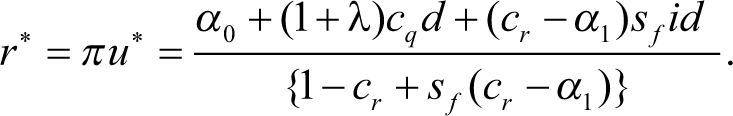
r^{*} = π u^{*} = \frac{α_{0} + (1 + λ) c_{q} d + (c_{r} - α_{1}) s_{f} i d}{{1 - c_{r} + s_{f} (c_{r} - α_{1})}}

(13)

2.2 Comparative Statics

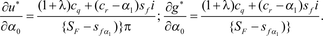
Differentiating partially u*, g* and r* with respect to α₀, we get

\frac{\partial u^{*}}{\partial α_{0}} = \frac{1}{{S_{F} - s_{f α_{1}})} π} > 0; \frac{\partial g^{*}}{\partial α_{0}} = \frac{S_{F}}{{S_{F} - s_{f α_{1}})}} > 0; \frac{\partial r^{*}}{\partial α_{0}} = \frac{1}{{S_{F} - s_{f α_{1}})}} > 0.

(14)

where S_F = 1 − c_r + s_fc_r > 0 and {S_F − s_fα₁)} = {1 − c_r + s_f(c_r − α₁)} > 0. Due to a rise in animal spirits (α₀), equilibrium degree of capacity utilization, growth rate and rate of profit all increase.

Partial differentiation of u* and r* with respect to d yields

\frac{\partial u^{*}}{\partial α_{0}} = \frac{(1 + λ) c_{q} + (c_{r} - α_{1}) s_{f} i}{{S_{F} - s_{f α_{1}})} π}; \frac{\partial g^{*}}{\partial α_{0}} = \frac{(1 + λ) c_{q} + (c_{r} - α_{1}) s_{f} i}{{S_{F} - s_{f α_{1}})}} .

(15)

If (c_r – α₁) > 0, the economy is always in a debt-led demand regime, that is, $\frac{\partial u^{*}}{\partial α_{0}} < 0$ But, if (c_r – α₁) < 0, then if (1 + λ)c_q < (c_r – α₁)s_fi, the economy is in a debt-burdened demand regime, that is, $\frac{\partial u^{*}}{\partial d} < 0.$ . Otherwise, it is in a debt-led demand regime. The movement in r* is in the same direction as u*. An increase in d, by reducing the available internal funds, reduces the investment demand by α₁s_fi unit (see Equation (7)). But the consumption demand of rentiers increases by {c_rs_fi + (1 + λ)c_q} unit (see Equation (6)). If the latter is higher than the former, then for a given amount of capital, the aggregate demand and hence the degree of capacity utilization rises.

Partial differentiation of g* with respect to d yields

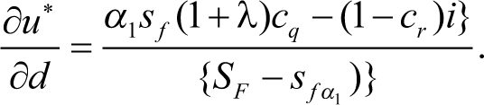
\frac{\partial u^{*}}{\partial d} = \frac{α_{1} s_{f} (1 + λ) c_{q} - (1 - c_{r}) i}}{{S_{F} - s_{f α_{1}})}} .

(16)

The economy is in a debt-led growth regime if and only if (1+ λ)c_q > (1 − c_r)i. Otherwise, it is in a debt-burdened growth regime. An increase in d affects the equilibrium growth rate in two ways. First, by reducing the available internal fund it directly negatively affects the growth rate. On the other hand, through its effect on the equilibrium degree of capacity utilization, it indirectly affects the equilibrium growth rate.⁹ In other words, we get the debt-led growth when the effect of aggregate demand from higher income of creditors more than offset the decrease in investment demand due to a higher debt burden, and in the opposite case the debt-burdened growth occurs.

Differentiating partially u*, g* and r* with respect to i, we get

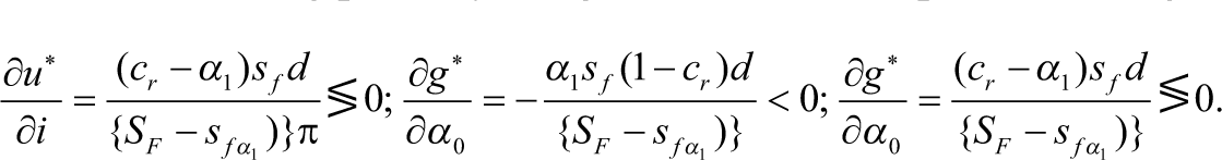
\frac{\partial u^{*}}{\partial i} = \frac{(c_{r} - α_{1}) s_{f} d}{{S_{F} - s_{f α_{1}})} π} > 0; \frac{\partial g^{*}}{\partial α_{0}} = - \frac{α_{1} s_{f} (1 - c_{r}) d}{{S_{F} - s_{f α_{1}})}} < 0; \frac{\partial g^{*}}{\partial α_{0}} = \frac{(c_{r} - α_{1}) s_{f} d}{{S_{F} - s_{f α_{1}})}} > 0.

(17)

An increase in the interest rate, by reducing the available internal funds, reduces the investment rate (i.e. investment-to-capital ratio) by a₁s_fd unit, whereas the consumption rate of rentiers (i.e. rentiers’ consumption-to-capital ratio) increases by c_rs_fd unit. If the latter is greater than the former, then, for a given amount of capital, the aggregate demand and hence the degree of capacity utilization rises.

A rise in the interest rate leads to a fall in the equilibrium rate of capital accumulation. The reason is twofold. First, by reducing internal funds, it directly negatively affects the growth rate. Second, through its effect on the equilibrium degree of capacity utilization, it indirectly affects the equilibrium growth rate. The latter effect¹⁰ is, however, smaller than the former. Therefore, the impact of a rise in the interest rate on the equilibrium rate of capital accumulation is always negative.

Differentiating partially u*, g* and r* with respect to λ, we get

\frac{\partial u^{*}}{\partial λ} = \frac{c_{q} d}{{S_{F} - s_{f α_{1}})} π} > 0; \frac{\partial g^{*}}{\partial λ} = \frac{α_{1} s_{f} c_{q} d}{{S_{F} - s_{f α_{1}})}} > 0; \frac{\partial r^{*}}{\partial λ} = \frac{c_{q} d}{{S_{F} - s_{f α_{1}})}} > 0.

(18)

Unlike the debt-to-capital ratio, for a given level of debt, an increase in the equity-to-debt ratio unambiguously increases the equilibrium degree of capacity utilization, the equilibrium rate of profit and the equilibrium growth rate. For a given level of debt, due to a rise in the equity-to-debt ratio (i.e. a rise in the total value of equity), the consumption rate of rentiers increases by c_qd unit, while there is no initial change in investment demand. Hence, the equilibrium degree of capacity utilization increases. Through its positive influence on u*, the equity-to-debt ratio positively affects the equilibrium growth rate.

Differentiating partially u*, g* and r* with respect to π, we get

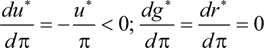
\frac{d u^{*}}{d π} = - \frac{u^{*}}{π} < 0; \frac{d g^{*}}{d π} = \frac{d r^{*}}{d π} = 0

(19)

Equation (19) explains that the economy is in a wage-led demand regime. This is because a rise in profit share (or a fall in wage share) distributes income from wage earners (who have a very high propensity to consume (c_w = 1)) to profit earners (who have a lower propensity to spend (c_r < 1)).

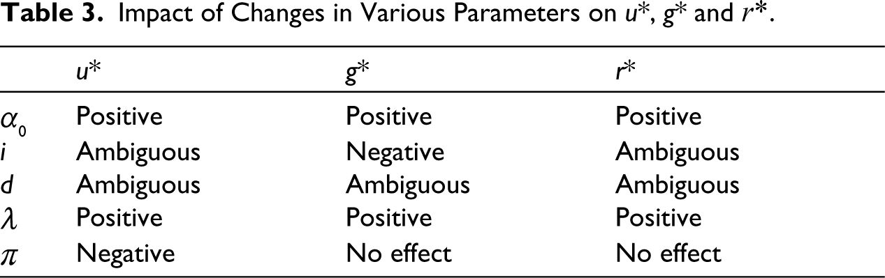
A rise in π, for a given value of u*, raises the investment rate by α₁s_fu* unit, whereas a rise in π, through its effect on u*, reduces the investment rate by exactly the same unit $(i . e . b y α_{1} s_{f} π \frac{\partial g^{*}}{\partial d_{0}} = α_{1} s_{f} u^{*} u n i t)$ Consequently, a rise in the profit share has no impact on the equilibrium growth rate.

The above-discussed short-run comparative static results are encapsulated in Table 3. In the next section, we proceed with the long-run dynamics.

Table 3.

Impact of Changes in Various Parameters on u*, g* and r*.

	u*	g*	r*
α ₀	Positive	Positive	Positive
i	Ambiguous	Negative	Ambiguous
d	Ambiguous	Ambiguous	Ambiguous
λ	Positive	Positive	Positive
π	Negative	No effect	No effect

Long Run

We analyse the long-run dynamics of the debt–capital ratio and equity-to-debt ratio in this section. In the long-run, we assume that the goods market always clears, i.e., equilibrium values of u, g and r are always attained. Note that the short-run is the time span in which the ratio of debt to capital and the ratio of equity to debt are both given, with these ratios (and hence the equilibrium values of the endogenous variables which adjust in the short-run, such as u, g and r) varying in the transition towards the long run. We assume the long-run equilibrium is attained when the debt–capital ratio (d) and the equity-debt ratio (λ) remain constant over time. Let us first focus on the dynamics of debt–capital ratio.

Dynamics of the Debt–Capital Ratio

We know that for business flows of funds, sources of funds must be equal to uses of funds, which in turn implies

retained earnings + new borrowings + issuance of new equities = investment demand

\Rightarrow s_{f} (π u - i d) K + D ˙ + P_{e} Ė = I .

(20)

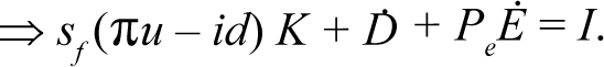
According to Ryoo (2010), debt finance is endogenously determined through the relationship between firms’ profitability and leverage ratio (i.e. the trend rate of corporate profitability-to-interest payment ratio) and the equity finance (x) is pure residual of firms’ financing constraint¹¹ as it serves as a buffer to fill the gap between the funds needed for the investment plans and the funds available from retained earnings and bank loans. However, it is very unlikely that funds needed for the investment plans of firms are lower than the available fund from retained earnings and borrowings for a sufficiently long period and the excess funds are adjusted by repurchasing stocks. Instead, there are various alternative and plausible explanations for stock buybacks. Lazonick (2010) points out:

‘the manifestation of the financialization of the U.S. economy is the obsession of corporate executives with distributing “value” to share holders, especially in the form of stock repurchases, even if they accomplish this goal at the expense of investment in innovation and the creation of U.S. employment opportunities’.

One of the central motives behind stock buybacks is investor exploitation. As long as market prices of stocks are below their ‘intrinsic’ values, firms try to buyback the stocks (see D’Mello & Shroff, 2000). Another motive is to remove low-valuation stockholders for mitigating the possibility of takeovers by other firms. Firms sometimes choose to buyback shares for increasing the reported EPS (earning per share) (Baker et al., 1985; Brav et al., 2005). Share buybacks can also be used to signal the management’s confidence about the future (Brav et al., 2005). As a result, it is more logical to assume that firms first decide how much of its investment is financed by the issuance of equities (or how much firms decide to spend for share buybacks) and then firms fill the gap between the funds needed and the funds available for the investment plans by debt financing. So instead of equity finance, it should be the debt finance as the accommodating variable.¹²

Figure 4.

Source: Bureau of Economic Analysis, 21 December 2018, Table 1.10; author’s calculations.

Figure 5.

Source: Bureau of Economic Analysis, 27 November 2024, Table 1.10; author’s calculations.

For simplicity, we assume a fraction of investment (x) is always financed by the issuance of equities,¹³ that is, instead of treating x as a variable we treat it as a parameter. This assumption is found in Lavoie and Godley (2002), Dos Santos and Zezza (2008), Taylor and Rada (2007) and Taylor (2012) etc. Solving Equation (1) for the change in debt–capital ratio as a quadratic function of debt–capital ratio itself, we get

\dot{d} = \frac{m - l d - h d^{2}}{S_{F} - s_{f} α_{1}}

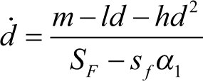
A diagram of the d˙ = 0 isocline is shown in Figure 6. Further investigation yields that the slope of the $\frac{d λ}{d d} |_{\dot{d} = 0} = \frac{α_{0} A (d - d^{'}) (d - d^{″})}{s_{f} c_{q} {[(1 - α_{1} + α_{1} x) d + α_{1} d^{2}]}^{2}} .$

Figure 6.

Diagrams of the Two Isoclines.

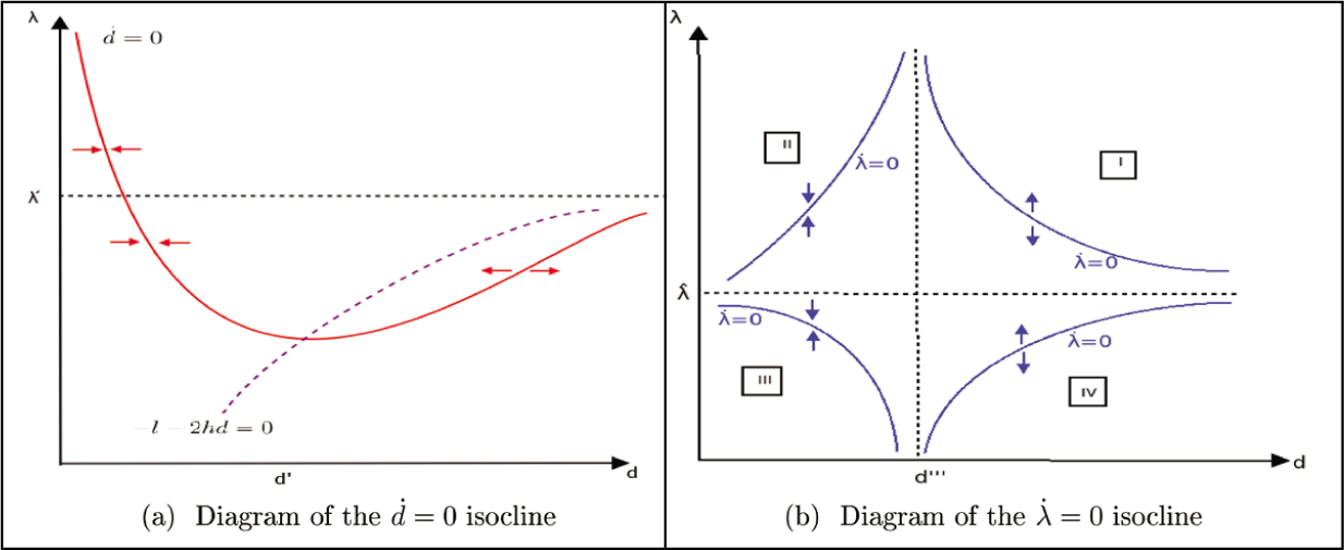
See Appendix A.1 for the derivation. Note that for the low values of debt–capital ratio (i.e. for d > d′), the linear term dominates the quadratic term and therefore we get a negatively sloped d˙ = 0 isocline. On the other hand, for a higher debt–capital ratio (i.e. for d > d′), the opposite happens. Consequently, we get a positively sloped d˙ = 0 isocline. Now we focus on the rentiers’ portfolio dynamics.

Dynamics of the Equity–Debt Ratio

We assume that the composition of households’ portfolio is affected by their views on stock market performance.

Let us assume

λ . = 0 [λ^{d} - λ]; θ > 0,

(21)

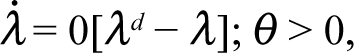
where λ^d is the desired equity-to-debt ratio of the rentiers. It depends on the expectation regarding future capital gain.¹⁴ θ represents the speed of the adjustment parameter. This speed of the adjustment parameter can be affected by, inter alia, the regulation of the financial market. A strictly regulated financial market is associated with a smaller value of θ.

According to Abdullah and Hayworth (1993), ‘The level of aggregate economic activity may influence stock prices through its impact on corporate profitability. An increase in output may increase cash flows and hence raise stock prices, while a recession would have the opposite effect’. Fama (1990) shows that the stock returns are highly correlated with the future production growth rates for the period 1953–1987 for the US economy. In his analysis, production growth rates explain 43% of the stock return variance. Future production growth, as he argues, reflects information about future cash flows, which in turn influence the stock prices. Schwert (1990) using 100 years of data (1889–1988) find a strong positive relationship between real stock returns and future production growth rates. In his analysis, the future production growth rate is capable of explaining a large fraction of the variation in stock returns. Ratanapakorn and Sharma (2007), using quarterly data between 1975 and 1999, found that industrial production positively influences the stock prices. As they argue, a rise in industrial production increases the corporate earnings and hence enhances the present value of the firm. This leads to a rise in the investment in the stock market and therefore enhances the stock prices. Naik and Padhi (2012) find a bidirectional causality between industrial production and stock prices for India for the period 1994-2011. Therefore, we assume the expected capital gain depends on the growth rate.¹⁵ In other words, the expectation of rentiers regarding future capital gain depends on economic growth. If the economy is performing well, they expect this to sustain for long, and they expect a sizeable future capital gain. So their desired equity-to-debt ratio (λ^d) increases.

Let us assume

λ^{d} = ε g; ε > 0,

(22)

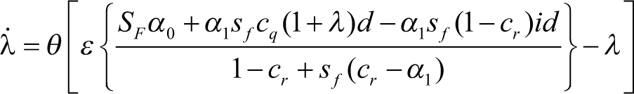
ε measures the sensitivity of the desired equity-to-debt ratio to a change in the growth rate. Equations (21) and (22) yield

λ . = θ [ε g - λ] .

From Equation (23), this implies that

\dot{λ} = θ [ε {\frac{S_{F} α_{0} + α_{1} s_{f} c_{q} (1 + λ) d - α_{1} s_{f} (1 - c_{r}) i d}{1 - c_{r} + s_{f} (c_{r} - α_{1})}} - λ]

(23)

\Rightarrow \dot{λ} = θ [\frac{S_{F} α_{0} ε + α_{1} s_{f} ε {c_{q} - (1 + c_{r}) i} d - [1 - c_{r} - s_{f} (c_{r} - α_{1}) - α_{1} s_{f} c_{q} ε d] λ}{1 - c_{r} + s_{f} (c_{r} - α_{1})}]

(24)

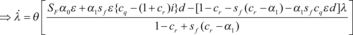
In equilibrium λ. = 0. Rearranging Equation (25), we get

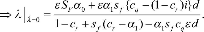
\Rightarrow λ |_{\dot{λ} = 0} = \frac{ε S_{F} α_{0} + ε α_{1} s_{f} {c_{q} - (1 - c_{r}) i} d}{1 - c_{r} + s_{f} (c_{r} - α_{1}) - α_{1} s_{f} c_{q} ε d} .

(25)

So putting d = 0 in Equation (25) we get the vertical intercept of the λ. = 0 isocline as 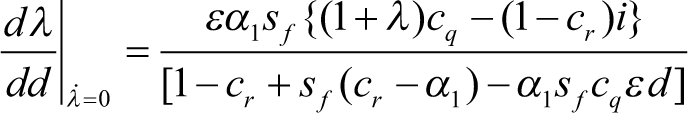$λ |_{\dot{λ} = 0}^{d = 0} = \frac{ε S_{F} α_{0}}{1 - c_{r} + s_{f} (c_{r} - α_{1})} > 0.$ Further investigation yields that the slope of the λ. = 0 isocline is

{\frac{d λ}{d d} |}_{\dot{λ} = 0} = \frac{ε α_{1} s_{f} {(1 + λ) c_{q} - (1 - c_{r}) i}}{[1 - c_{r} + s_{f} (c_{r} - α_{1}) - α_{1} s_{f} c_{q} ε d]}

(26)

Depending on the values of d and λ, we get positively or negatively sloped λ. = 0 isoclines as depicted in Figure 6b. See Appendix A.2 for the mathematical derivation.

Jacobian Elements of the System

We get that $J_{11} = \frac{\partial \dot{d}}{\partial d} \frac{>}{<} 0, J_{12} = \frac{\partial \dot{d}}{\partial λ} < 0, J_{21} = \frac{\partial \dot{d}}{\partial λ} \frac{>}{<} 0 and J_{22} = \frac{\partial \dot{λ}}{\partial λ} \frac{>}{<} 0$ . See Appendix A.2 for the detailed calculation. Note that for {(1 + λ)c_q − (1 − c_r)i} > 0, that is, when the economy is in a debt-led growth regime, J₁₁ is unambiguously negative, and therefore, the d˙ = 0 isocline is negatively sloped (as J₁₂ is always negative). However, for {(1 + λ)c_q − (1 − c_r)i} < 0, that is, when the economy is in a debt-burdened growth regime, for smaller values of d $(as long as d < \frac{- 1}{2 h})$ , J₁₁ < 0 and therefore the d˙ = 0 isocline is negatively sloped. On the other hand, for a higher values of $d (\forall d > \frac{- 1}{2 h})$ J₁₁ > 0 and therefore the slope of the d˙ = 0 isocline is positive. λ. = 0 isocline is vertically asymptotic at $d^{‴} = \frac{1 - c_{r} + s_{f} (c_{r} - α_{1})}{α_{1} s_{f} c_{q} ε}$ > 0. Figure 6a represents the d• = 0 isocline. From the preceding discussion, the following proposition can be inferred.

Proposition 1. When the economy is in a debt-led growth regime, irrespective of the level of debt–capital ratio, J ₁₁ becomes negative. However, in case of a debt-burdened growth regime, $j_{11} \frac{>}{<} 0$ according to whether $d \frac{>}{<} - \frac{1}{2 h} .$

Possible Cases

In this section, we explain different possible cases which may arise due to the interaction between the debt and the portfolio dynamics. Depending on whether the economy is in a debt-led or a debt-burdened growth regime, we can have four possible cases. We analyse case 1 here. Rest of the cases along with the possibility of Hopf bifurcation are discussed in Appendices B and C.

Case 1

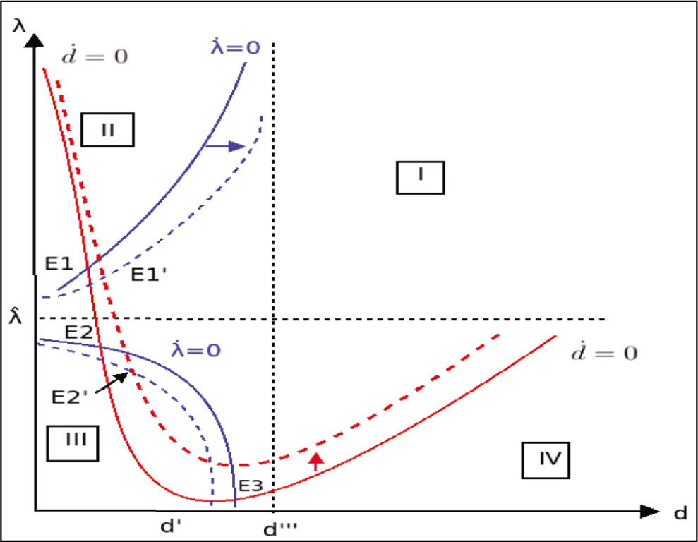
As illustrated in Figure 7, in case 1, the d˙ = 0 isocline is passing through quadrants II, III and IV. However, slope of the d˙ = 0 isocline changes its sign in the III quadrant. In case 1, therefore, d′ < d″′. In the II quadrant we get only one steady-state named E₁. There may be two equilibria named E₂ and E₃ in the III quadrant while two equilibria named E₄ and E₅ are possible in the IV quadrant. So, maximum five different equilibria are pos sible in case 1.

Figure 7.

Case 1.

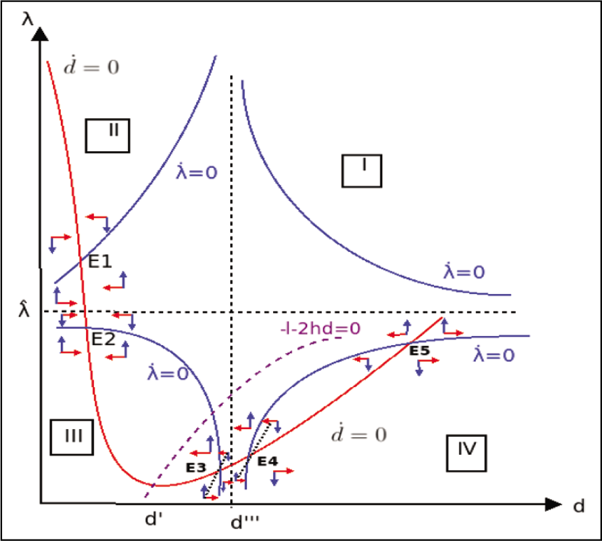
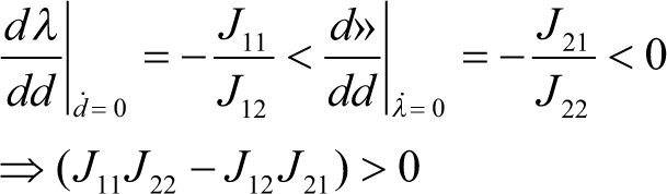
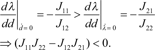
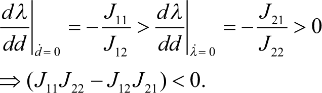
Consider point E₁: Here the economy is in a debt-led growth regime (as λ > λˆ). λ > λˆ and Equation (A.7) implies J₂₁ > 0, whereas λ > λˆ and Equation (A.10) implies J₁₁ < 0. As d < d″′, Equation (A.8) yields that J₂₂ < 0. J₁₂ is always negative. Thus at E₁, the determinant of the Jacobian matrix is positive $(asDet (j) (\bar{\overset{︷}{j_{11}}} \bar{\overset{︷}{j_{22}}} - \bar{\overset{︷}{j_{12}}} \bar{\overset{︷}{j_{21}}}) > 0)$ , and the trace of the Jacobian matrix is negative $(tr(J)=(\bar{\overset{︷}{J_{11}}} + \bar{\overset{︷}{J_{22}}})<0)$ . Hence, point E₁ is a stable steady-state.

Let us explain the stability of the steady-state E₁ intuitively. Because of some exogenous shock, let us assume that the debt–capital ratio deviates from its steady-state value. Suppose that the debt–capital ratio is greater than its steady-state value. First, in the debt-led growth regime, if d is greater than the steady-state value d*, it must fall due to $\frac{\partial \dot{d}}{\partial d} = J_{11} < 0.$ This is the direct effect. Second, as the debt–capital ratio is greater than its steady-state value, the equity-debt ratio increases due to J₂₁ > 0. This leads to a fall in the debt–capital ratio due to J₁₂ < 0. This is the indirect effect. In the debt-led growth regime, both the direct and indirect effects are stable. As a result, in this case, if the debt–capital ratio rises from the steady-state value, it again comes back to its steady-state. Hence, the steady-state is stable.

Consider point E₂: At the steady-state E₂, the economy is in a debt-burdened growth regime (i.e. λ < λˆ here). λ < λˆ and Equation (A.7) implies J₂₁ < 0. Slope of the d˙ = 0 isocline is negative here, that is, ${\frac{d λ}{d d} |}_{\dot{d} = 0} = - \frac{J_{11}}{J_{12}} < 0$ At J₁₂ < 0, J₁₁ must be negative then.¹⁶ At E₂, the debt–capital ratio is so small that d < d^″′. Equation (A.8) and d < d″′ together implies J₂₂ < 0. At point E₂, slope of the d˙ = 0 isocline is less than the slope of the λ. = 0 isocline, that is,

\begin{array}{l} {\frac{d λ}{d d} |}_{\dot{d} = 0} = - \frac{J_{11}}{J_{12}} < {\frac{d λ}{d d} |}_{\dot{λ} = 0} = - \frac{J_{21}}{J_{22}} < 0 \\ \Rightarrow (J_{11} J_{22} - J_{12} J_{21}) > 0 \end{array}

Therefore, the determinant is positive, and the trace is negative (tr(J) = J₁₁ + J₂₂ < 0). So point E₂ is a stable steady-state.

Debt–capital ratio, suppose due to some reason, deviates from the steady-state and is now lower than its steady-state value. There exist two opposite effects near E₂. First, as the debt–capital ratio is lower than its steady-state value, it must rise due to $\frac{\partial \dot{d}}{\partial d} = J_{11} < 0.$ This is the direct stable effect. Second, the fall in debt–capital ratio leads to a rise in the equity-debt ratio due to J₂₁ < 0. As J₁₂ < 0, this rise in equity-debt ratio leads to a fall in the debt–capital ratio. This second effect is an indirect unstable effect. However, as λ is very close to λˆ near E₂, the magnitude of {(1 + λ)c_q − (1 − c_r)i} is very small in size. Therefore, the negative effect of J₂₁ is very weak (see Figure 7 and Equation (7)). As a result, the fall in the debt–capital ratio leads to a small amount of rise in the equity-debt ratio which in turn through Equation (A.11) leads to a negligible amount of fall in the debt–capital ratio (as d is low near E₂, the negative effect of J₁₂ is very weak too). Therefore, the direct stable effect dominates the indirect unstable effect and results in the steady-state to be stable.

Consider point E₃: As at E₃ λ < λˆ, the economy is in a debt-burdened growth regime and J₂₁ < 0. As $d > \frac{- 1}{2 h}, J_{11} > 0.$ At E₃, the debt–capital ratio is so small that d < d″′. Equation (A.8) and d < d′″ together imply J₂₂ < 0. At point E₃, slope of the d˙ = 0 isocline is greater than the slope of the λ. = 0 isocline, that is,

\begin{array}{l} {\frac{d λ}{d d} |}_{\dot{d} = 0} = - \frac{J_{11}}{J_{12}} > {\frac{d λ}{d d} |}_{\dot{λ} = 0} = - \frac{J_{21}}{J_{22}} \\ \Rightarrow (J_{11} J_{22} - J_{12} J_{21}) < 0. \end{array}

Hence, the determinant is negative. Consequently, E₃ emerges as a saddle point.

Let us discuss it intuitively. The equity–debt ratio, suppose due to some reason, deviates from the steady-state and is now lower than its steady-state value. There exist two

opposite effects near the steady-state E₃. First, as the equity-debt ratio is lower than its steady-state value, it must rise due to J₂₂ < 0. This is the direct stable effect. However, as d is close to d^″′, the negative effect of J₂₂ is very weak (see Figure 7 and Equation (A.8)). As a result, the initial fall in the equity-debt ratio leads to a small rise in the equity-debt ratio. Second, the fall in equity-debt ratio leads to a rise in the debt–capital ratio due to J₁₂ < 0. As J₂₁ < 0, this rise in debt–capital ratio leads to a fall in the equity-debt ratio. This second effect is an indirect unstable effect. However, as the gap between λ and λˆ is high near E₃, the magnitude of {(1 + λ)c_q − (1 − c_r)i} is large in size. Therefore, the negative effect of J₂₁ is strong (see Figure 7 and Equation (A.7)). As a result, the rise in debt–capital ratio leads to a large amount of fall in the equity-debt ratio. Consequently, the indirect unstable effect dominates the direct stable effect and results in the steady-state to be unstable. There is only one stable arm that reaches the equilibrium point E₃. Hence, E₃ emerges as a saddle point.

Consider point E₄: At the steady-state E₄, the economy is in a debt-burdened growth regime and here $J_{21} < 0. d > \frac{- l}{2 h}$ implies J₁₁ > 0. d > d′″ implies (from Equation (A.8)) J₂₂ > 0. At point E₄, slope of the λ˙ = 0 isocline is greater than the slope of the d˙ = 0 isocline, that is,

\begin{array}{l} {\frac{d λ}{d d} |}_{\dot{λ} = 0} = - \frac{J_{21}}{J_{22}} > {\frac{d λ}{d d} |}_{\dot{d} = 0} = - \frac{J_{11}}{J_{12}} > 0 \\ \Rightarrow (J_{11} J_{22} - J_{12} J_{21}) < 0. \end{array}

As the determinant is negative, E₄ is a saddle point.

Suppose due to some reason, the equity-debt ratio deviates from the steady-state and is now higher than its steady-state value. First, as the equity-debt ratio is higher than its steady-state value, it must rise due to J₂₂ > 0. Second, the rise in the equity-debt ratio leads to a fall in the debt–capital ratio due to J₁₂ < 0. As J₂₁ < 0, this fall in debt–capital ratio leads to a rise in the equity-debt ratio. So, both the effects are unstable. Consequently, the steady-state is unstable. There is only one stable arm that reaches the equilibrium point E₄. Hence, E₄ emerges as a saddle point.

Consider point E₅: Here the economy is in a debt-burdened growth regime. Consequently, J₂₁ < 0. On the other hand, d > d′″ and, therefore, J₂₂ < 0. $As d > \frac{- 1}{2 h}, J_{11} > 0.$ At point E₅, the slope of the d˙ = 0 isocline is greater than the slope of the λ. = 0 isocline, that is,

\begin{array}{l} {\frac{d λ}{d d} |}_{\dot{d} = 0} = - \frac{J_{11}}{J_{12}} > {\frac{d λ}{d d} |}_{\dot{λ} = 0} = - \frac{J_{21}}{J_{22}} > 0 \\ \Rightarrow (J_{11} J_{22} - J_{12} J_{21}) < 0. \end{array}

Both the determinant and the trace (tr(J) = J₁₁ + J₂₂ > 0) are positive here. So point E₅ is an unstable steady-state.

Let us discuss it intuitively. Equity-debt ratio, suppose due to some reason, deviates from the steady-state and is now lower than its steady-state value. There exist two opposite effects near the steady-state E₅. First, as the equity-debt ratio is lower than its steady-state value, it must fall due to J₂₂ > 0. This is the direct unstable effect. Second, the fall in the equity-debt ratio leads to a rise in the debt–capital ratio due to J₁₂ < 0. As J₂₁ < 0, this rise in the debt–capital ratio leads to a fall in the equity-debt ratio. This second effect is also an indirect unstable effect. Consequently, E₅ is an unstable steady-state.

In case 1, instead of E₂ and E₃, a new equilibrium E₈, and instead of E₄ and E₅, a new equilibrium E₉ are also possible. As illustrated in Figure 8, E₈ and E₉ are both saddle-point unstable steady-states.

Figure 8.

Case 1: When d˙ = 0 and λ. = 0 Isoclines are Tangent at III and IV Quadrants.

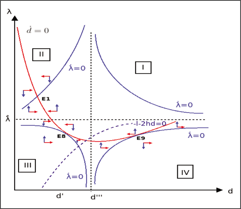
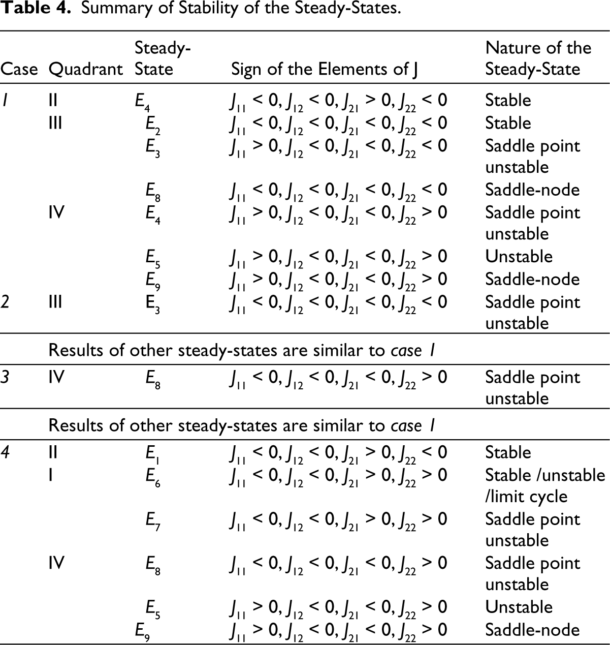
Table 4 summarizes the results of the stability related to various steady-states. From the analysis of the fourth section, two points are worth remembering.

Table 4.

Summary of Stability of the Steady-States.

Case	Quadrant	Steady-State	Sign of the Elements of J	Nature of the Steady-State
1	II	E ₄	J₁₁ < 0, J₁₂ < 0, J₂₁ > 0, J₂₂ < 0	Stable
	III	E ₂	J₁₁ < 0, J₁₂ < 0, J₂₁ < 0, J₂₂ < 0	Stable
		E ₃	J₁₁ > 0, J₁₂ < 0, J₂₁ < 0, J₂₂ < 0	Saddle point unstable
		E ₈	J₁₁ < 0, J₁₂ < 0, J₂₁ < 0, J₂₂ < 0	Saddle-node
	IV	E ₄	J₁₁ > 0, J₁₂ < 0, J₂₁ < 0, J₂₂ > 0	Saddle point unstable
		E ₅	J₁₁ > 0, J₁₂ < 0, J₂₁ < 0, J₂₂ > 0	Unstable
		E ₉	J₁₁ > 0, J₁₂ < 0, J₂₁ < 0, J₂₂ > 0	Saddle-node
2	III	E₃	J₁₁ < 0, J₁₂ < 0, J₂₁ < 0, J₂₂ < 0	Saddle point unstable
	Results of other steady-states are similar to case 1
3	IV	E ₈	J₁₁ < 0, J₁₂ < 0, J₂₁ < 0, J₂₂ > 0	Saddle point unstable
	Results of other steady-states are similar to case 1
4	II	E ₁	J₁₁ < 0, J₁₂ < 0, J₂₁ > 0, J₂₂ < 0	Stable
	I	E ₆	J₁₁ < 0, J₁₂ < 0, J₂₁ > 0, J₂₂ > 0	Stable /unstable /limit cycle
	I	E ₇	J₁₁ < 0, J₁₂ < 0, J₂₁ > 0, J₂₂ > 0	Saddle point unstable
	IV	E ₈	J₁₁ < 0, J₁₂ < 0, J₂₁ < 0, J₂₂ > 0	Saddle point unstable
		E ₅	J₁₁ > 0, J₁₂ < 0, J₂₁ < 0, J₂₂ > 0	Unstable
		E ₉	J₁₁ > 0, J₁₂ < 0, J₂₁ < 0, J₂₂ > 0	Saddle-node

Remark 1. If the economy is in a debt-led growth regime, a lower level of debt–capital ratio (i.e. d < d^″′) is a sufficient condition for achieving the unique stable steady-state. However, it is not a necessary condition for achieving stability (for example see E₆ of case 4, Figure B.6).

Remark 2. When the economy is in a debt-burdened growth regime, a lower level of debt–capital ratio $(i . e, d < - \frac{l}{2 h})$ is a necessary (although not sufficient) condition for achieving the stable steady-state (see E₂ of case 1, Figure 7).¹⁷

Comparative Statics

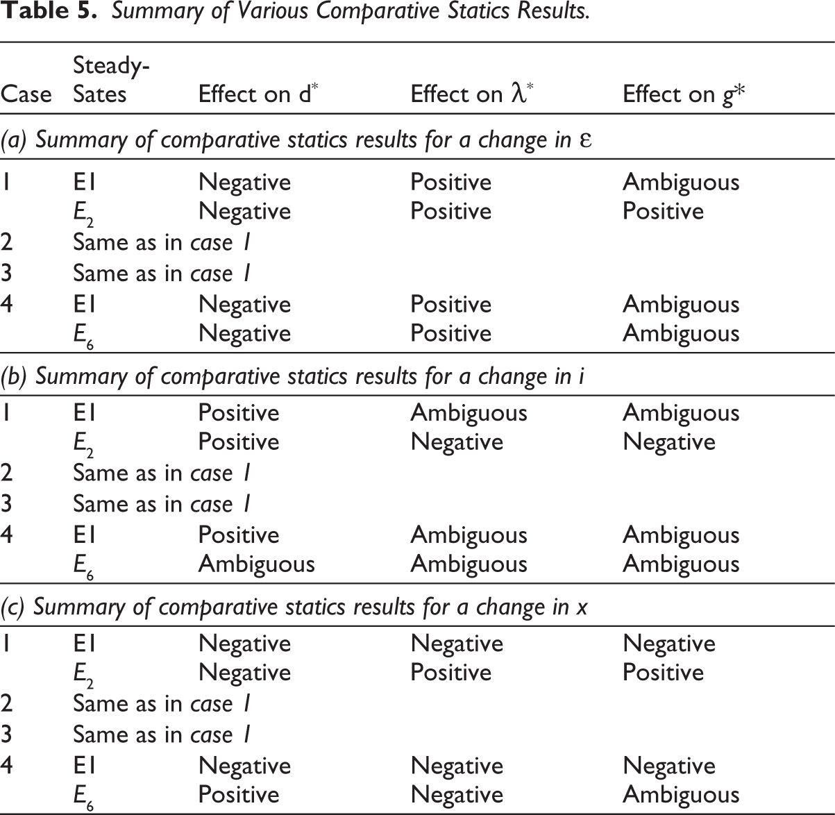
In this section, we investigate how various parameters influence the equilibrium values of the debt–capital ratio and the equity-debt ratio. Table 5 summarizes the results of the comparative statics.

Table 5.

Summary of Various Comparative Statics Results.

Case	Steady-Sates	Effect on d^*	Effect on λ^*	Effect on g*
(a) Summary of comparative statics results for a change in ε
1	E1 E₂	Negative Negative	Positive Positive	Ambiguous Positive
2	Same as in case 1
3	Same as in case 1
4	E1 E₆	Negative Negative	Positive Positive	Ambiguous Ambiguous
(b) Summary of comparative statics results for a change in i
1	E1 E₂	Positive Positive	Ambiguous Negative	Ambiguous Negative
2	Same as in case 1
3	Same as in case 1
4	E1 E₆	Positive Ambiguous	Ambiguous Ambiguous	Ambiguous Ambiguous
(c) Summary of comparative statics results for a change in x
1	E1 E₂	Negative Negative	Negative Positive	Negative Positive
2	Same as in case 1
3	Same as in case 1
4	E1 E₆	Negative Positive	Negative Negative	Negative Ambiguous

The total differentiation of Equations (A.9) and (3.5) shows the effects of parametric changes in the economy which imply

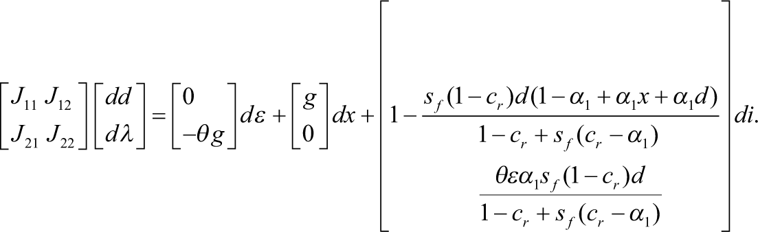
[\begin{array}{l} J_{11} J_{12} \\ J_{21} J_{22} \end{array}] [\begin{array}{l} d d \\ d λ \end{array}] = [\begin{array}{l} 0 \\ - θ g \end{array}] d ε + [\begin{array}{l} g \\ 0 \end{array}] d x + [1 - \frac{s_{f} (1 - c_{r}) d (1 - α_{1} + α_{1} x + α_{1} d)}{\begin{array}{l} 1 - c_{r} + s_{f} (c_{r} - α_{1}) \\ \frac{θ ε α_{1} s_{f} (1 - c_{r}) d}{1 - c_{r} + s_{f} (c_{r} - α_{1})} \end{array}}] d i .

(27)

Frome Equation (5.1), we get $\begin{array}{l} \frac{d d *}{d ε} = \frac{θ g * J_{12}}{(J_{11} J_{22} - J_{12} J_{21})}, \frac{d λ *}{d ε} = \frac{- θ g * J_{11}}{(J_{11} J_{22} - J_{12} J_{21})}; \frac{d d *}{d x} = \frac{g * J_{22}}{(J_{11} J_{22} - J_{12} J_{21})}, \\ \frac{d λ *}{d x} = \frac{- g * J_{21}}{(J_{11} J_{22} - J_{12} J_{21})}; \frac{d d *}{d i} = \frac{\frac{s_{f} (1 - c_{r}) d (1 - α_{1} + α_{1} x + α_{1} d)}{1 - c_{r} + s_{f} (c_{r} - α_{1})} J_{22} - \frac{θ ε α_{1} s_{f} (1 - c_{r}) d}{1 - c_{r} + s_{f} (c_{r} - α_{1})} J_{12}}{(J_{11} J_{22} - J_{12} J_{21})}, \end{array}$ $\frac{d λ *}{d i} = \frac{\frac{θ ε α_{1} s_{f} (1 - c_{r}) d}{1 - c_{r} + s_{f} (c_{r} - α_{1})} J_{11} + \frac{s_{f} (1 - c_{r}) d (1 - α_{1} + α_{1} x + α_{1} d)}{1 - c_{r} + s_{f} (c_{r} - α_{1})} J_{21}}{(J_{11} J_{22} - J_{12} J_{21})}$ Note that for comparative static, the analysis of cases 2 and 3 is are the same as in case 1. We discuss the comparative statics related to case 4 in Appendix D. Therefore, we focus only on case 1 here.

Effect of a Change in ε

Here only two equilibria are stable: E₁ and E₂.

Consider point E₁: As illustrated in Figure 9, for a rise in ε, the vertical intercept of the λ. = 0 isocline rises, and the slope of the λ. = 0 isocline becomes steeper. Besides, the vertical asymptote decreases.¹⁸ However, there is no change in the d˙ = 0 isocline. Consequently, d^* decreases and λ^* increases.

Figure 9.

Effect of a Rise in ε: Case 1.

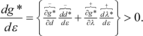
The economic intuition behind the fall in d^* and the rise in λ^* is as follows. A rise in ε, ceteris paribus, raises the desired equity-debt ratio of rentiers and thereby pushes the λ. = 0 isocline upwards. For a given λ, at the old steady-state E₁, the debt–capital ratio is higher than required for λ. = 0 to be satisfied. As the economy is in a debt-led growth regime, this higher level of d puts upward pressure on equity-debt ratio through Equation (A.7). As a result, equity-debt ratio (λ) starts rising. As soon as λ rises, the debt market deviates from its equilibrium position. Given the level of d, λ is now higher than required for d˙ = 0 to be satisfied. As ∂ d˙ ∂λ = J12 < 0, the debt–capital ratio must fall. The combination of a higher equity-debt ratio and a lower debt–capital ratio ultimately ensures to achieve the new equilibrium point E^′1 either monotonically or spiralling around E₁.

As demonstrated in Equation (5.2), at E₁, ε has an ambiguous effect on the long-run equilibrium rate of capital accumulation:

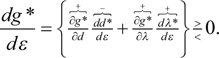
\frac{d g *}{d ε} = {\frac{\overset{+}{\overset{︷}{\partial g *}}}{\partial d} \frac{\bar{\overset{︷}{d d *}}}{d ε} + \frac{\overset{+}{\overset{︷}{\partial g *}}}{\partial λ} \frac{\overset{+}{\overset{︷}{d λ *}}}{d ε}} \frac{>}{<} 0.

(28)

At E₁, as ε increases, λ^* increases, which in turn enhances the equilibrium rate of capital accumulation. On the other hand, a rise in ε decreases d^*, and so g* declines. Hence, the final result of a rise in ε on g* is ambiguous.

Consider point E₂: For a rise in ε, the vertical intercept of the λ. = 0 isocline rises, while the λ. = 0 isocline becomes steeper.¹⁹ At E₂, a rise in ε leads to a rise in λ^* and a fall in d^*. At E₂, ε has an overall positive effect on the long-run equilibrium rate of capital accumulation (see Equation (5.3)).

\frac{d g *}{d ε} = {\frac{\bar{\overset{︷}{\partial g *}}}{\partial d} \frac{\bar{\overset{︷}{d d *}}}{d ε} + \frac{\overset{+}{\overset{︷}{\partial g *}}}{\partial λ} \frac{\overset{+}{\overset{︷}{d λ *}}}{d ε}} > 0.

(29)

At E₂, as ε increases, λ^* increases, which in turn enhances the equilibrium rate of capital accumulation. In addition, a rise in ε decreases d^*. As the economy is in a debt-burdened growth regime, a fall in d^* in turn raises g*. Hence, ε has an overall expansionary effect on the long-run equilibrium rate of capital accumulation. Thus, when the economy is in a relatively weak debt-burdened growth regime (as λ and λˆ are close to each other at E₂), and the debt–capital ratio is relatively low $(as d < \frac{- 1}{2 h} and d < d^{‴} at E_{2}),$ a rise in ε, the extent to which the rate of capital accumulation stimulates the desired equity–deposit ratio of rentiers, raises the equilibrium rate of capital accumulation in the long run.

Effect of a Change in the Rate of Interest, i

Consider point E₁: As illustrated in Figure 10, for a rise in the interest rate, the d˙ = 0 curve shifts upwards, whereas the λ. = 0 isocline becomes flatter.²⁰ Therefore, we get $\frac{d d *}{d i} > 0 and \frac{d λ *}{d i} \frac{>}{<} 0$ Interest rate has only a direct negative effect on g* in the short-run. However, as demonstrated in Equation (5.4), at E₁, i has an ambiguous effect on the long-run equilibrium rate of capital accumulation.

Figure 10.

Effect of a rise in i: case 1

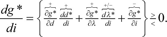
\frac{d g *}{d i} = {\frac{\overset{+}{\overset{︷}{\partial g *}}}{\partial d} \frac{\overset{+}{\overset{︷}{d d *}}}{d i} + \frac{\overset{+}{\overset{︷}{\partial g *}}}{\partial λ} \frac{\overset{+ / -}{\overset{︷}{d λ *}}}{d i} + \frac{\bar{\overset{︷}{\partial g *}}}{\partial i}} \frac{>}{<} 0.

(30)

At E₁, as i increases, d increases, which in turn enhances the equilibrium rate of capital accumulation (because here the economy is in a debt-led growth regime). On the other hand, interest rate has an ambiguous effect on λ^* while λ^* has a positive effect on g*. Finally, interest rate has a direct negative effect on the equilibrium rate of capital accumulation. Hence, the final result of a rise in i on g* is ambiguous. Note the stark difference between the impact of a change in the interest rate on the equilibrium rate of capital accumulation in the short-run and long run. A rise in the interest rate always leads to a fall in the equilibrium rate of capital accumulation in the short-run. This is because the direct effect of it on reducing the internal funds dominates the indirect effect through the equilibrium degree of capacity utilization in the short-run (which is captured by the term $\frac{\partial g *}{\partial i}$ in Equation (5.4)). However, apart from this direct effect, a change in the interest rate affects the equilibrium values of the debt–capital ratio and the equity-debt ratio in the long-run. These in turn have additional effects on the equilibrium rate of capital accumulation in the long-run.

Consider point E₂: Because of a rise in the interest rate, the d˙ = 0 curve shifts upwards. However, the λ. = 0 isocline becomes steeper.²¹ As a result, as shown in Figure 10, a rise in the interest rate leads to a rise in d* and a fall in λ*. At E₂, i has a vividly negative effect on the long-run equilibrium rate of capital accumulation. At E₂, as i increases, d increases, which in turn reduces the equilibrium rate of capital accumulation (because the economy is in a debt-burdened growth regime). On the other hand, the interest rate has a negative effect on λ^*, while λ^* has a positive effect on g*. So, a rise in i, through its negative effect on λ, decreases g* indirectly. Finally, the interest rate has a direct negative effect on the equilibrium rate of capital accumulation. Hence, the final result of a rise in i on g* is unequivocally negative (see (5.5)).

\frac{d g *}{d i} = {\frac{\bar{\overset{︷}{\partial g *}}}{\partial d} \frac{\overset{+}{\overset{︷}{d d *}}}{d i} + \frac{\overset{+}{\overset{︷}{\partial g *}}}{\partial λ} \frac{\bar{\overset{︷}{d λ *}}}{d i} + \frac{\bar{\overset{︷}{\partial g *}}}{\partial i}} < 0.

(31)

Effect of a Change in the Fraction of Investment Which is Financed by Issuance of New Equities, x

Consider point E₁:

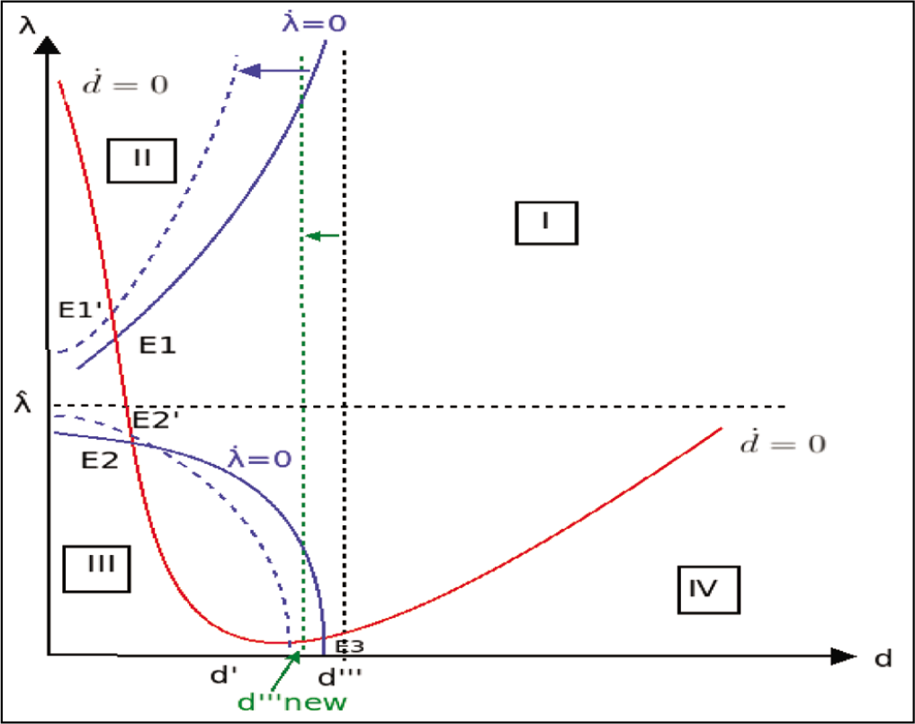
As depicted in Figure 11, for a fall in x, that is, when ‘share buyback’ happens, d˙ = 0 isocline shifts upwards. However, x has no impact on the λ. = 0 isocline.²² Therefore, as x increases, d* and λ* both decrease, whereas a fall in x leads to a rise in both λ* and d^*.

Figure 11.

Effect of a Fall in x: Case 1.

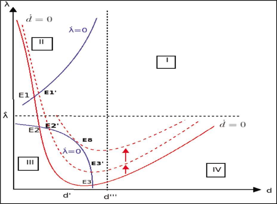
The economic intuition is as follows. If x decreases, that is, when the phenomenon called ‘share buyback’ happens, for the same level of investment, ceteris paribus, now firms get less funds through the issuance of new equities and as a result the d˙ = 0 isocline shifts upwards. For a given λ, at the old steady-state E₁, the debt–capital ratio is lower than required for new d˙ = 0 to be satisfied. 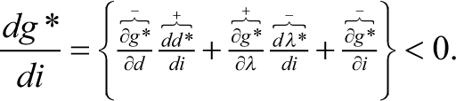$As \frac{\partial \dot{d}}{\partial d} = J_{11} < 0,$ the debt–capital ratio starts rising. As soon as d rises, λ. = 0 is no more satisfied. Given the level of λ, d is now higher than required for λ. = 0 to be satisfied. $As \frac{\partial λ}{\partial d} = J_{21} > 0,$ the equity-debt ratio also starts rising. The combination of a higher equity-debt ratio and a higher debt–capital ratio ultimately ensures to achieve the new equilibrium point E^′1 either monotonically or spiralling around E₁.

As demonstrated in Equation (5.6), at E₁, x has an unequivocally negative effect on the long-run equilibrium rate of capital accumulation.

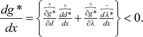
\frac{d g *}{d x} = {\frac{\overset{+}{\overset{︷}{\partial g *}}}{\partial d} \frac{\overset{+}{\overset{︷}{d d *}}}{d x} + \frac{\overset{+}{\overset{︷}{\partial g *}}}{\partial λ} \frac{\bar{\overset{︷}{d λ *}}}{d x}} < 0.

(32)

At E₁, as x increases, λ* decreases and as a result g* falls. On the other hand, a rise in x decreases d*. As the economy is in a debt-led growth regime, this fall in d^* reduces g*.

Hence, the final result of a rise in x on g* is vividly negative. Thus, when the economy is in a debt-led growth regime and the debt–capital ratio is significantly low $(as d < \frac{- 1}{2 h} and d < d^{‴} at E_{1}),$ repurchases of equities by firms (i.e. a fall in x) stimulates the equilibrium rate of capital accumulation in the long run.

Consider point E₂: Here $\frac{d d^{*}}{d x} < 0 a n d \frac{d λ^{*}}{d x} > 0.$ Thus, as x increases, d^* decreases and λ* increases, and when x decreases, λ^* decreases while d^* increases (see Figure 11). The reason is as follows. If x increases, for the same level of investment, ceteris paribus, now firms get more funds through the issuance of new equities, and as a result d falls (as now d˙ < 0). As here the economy is in a debt-burdened growth regime, for a fall in d, g*, which in turn raises the desired level of equity-debt ratio. Hence, the equilibrium equity-debt ratio rises too. The opposite happens for a fall in x (i.e. when ‘share buybacks’ happens).

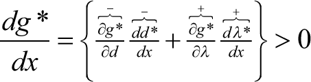
A rise in x has an unambiguously positive effect on the long-run equilibrium rate of capital accumulation at E₂. As x increases, λ^* rises, which in turn boosts g*. On the other hand, a rise in x reduces d^*. As the economy is in a debt-burdened growth regime, this fall in d^* in turn enhances g*g*. Hence, the final result of a rise in x on g* is vividly positive.

\frac{d g *}{d x} = {\frac{\bar{\overset{︷}{\partial g *}}}{\partial d} \frac{\bar{\overset{︷}{d d *}}}{d x} + \frac{\overset{+}{\overset{︷}{\partial g *}}}{\partial λ} \frac{\overset{+}{\overset{︷}{d λ *}}}{d x}} > 0

(33)

Note that for a decrease in x, the two equilibria E₂ and E₃ come closer and for a sufficient fall in x, both the equilibria converge to a unique saddle-point unstable steady-state E₈. Thus, in the era of financialization, as more of a share buyback is happening (and less proportion of investment is financed through issuance of new equities), when the economy is in a debt-burdened growth regime and the debt–capital ratio is low $(i .e . when d < \frac{- 1}{2 h} and d < d^{‴})$ not only the equilibrium rate of capital accumulation declines, the stable equilibrium E₂ may lose its stability as well in the sense that, at all, no stable steady-state exists in the economy.

In the post-Keynesian/neo-Kaleckian tradition, we observe two important paradoxes: ‘Keynes’ paradox of thrift’, in which a higher saving rate leads to a fall in output, and the ‘Kaleckian paradox of costs’, in which a higher real wage leads to a rise in the profit rate. However, in our analysis, we uncover a new paradox, say, the ‘paradox of share repurchases (or buybacks)’. For instance, consider the steady-state E₁ in case 1 in Figure 11, that is, when the economy is in a debt-led growth regime. A fall in x, which represents the occurrence of share buybacks, and hence a higher (respectively lower) fraction of investment being financed by debt (respectively issuance of equities), leads to a higher instead of lower ratio of equity to debt in the long-run equilibrium.

Conclusion

In this article, we investigated the post-COVID-19 firms’ debt dynamics and rentiers’ portfolio dynamics as coupled dynamics of the US economy considering a stock-flow consistent neo-Kaleckian growth model in which we endo-genize the debt–capital ratio and the equity-debt ratio. First, we examined the short-run stability and comparative statics. This article presents in great detail the dynamic properties of a neo-Kaleckian model, which allows for the possibility of a debt-led growth, when the effect of aggregate demand from higher income of creditors more than offsets the decrease in investment demand due to a higher debt burden. In the opposite case, the debt-burdened growth occurs. Thus, we concluded that although the economy is in a wage-led demand regime, debt-led or debt-burdened demand and growth regimes are possible. In the long run, we endogenize the equity-debt ratio and the debtcapital ratio. The coupled dynamics of firms’ debt and rentiers’ portfolio dynamics involve nonlinearities making the emergence of multiple equilibria possible with different stability properties which are carefully explored in the debt-led growth, including through a bifurcation analysis showing the possibility of the emergence of limit cycles. One innovative and laudable feature of the model is that firms can perform share repurchases, or buybacks, meaning that they can buy back their own shares from the marketplace. Such share repurchases impact both the long-run equilibrium rates of capacity utilization and output growth and the stability properties of the several long-run equilibrium configurations. The interesting results we found are as follows.

If the economy is in a debt-led growth regime, a lower level of debt–capital ratio is sufficient for achieving a unique stable steady-state. On the other hand, when the economy is in a debt-burdened growth regime, a lower level of debt–capital ratio is a necessary (although not sufficient) condition for achieving a stable steady-state.

Irrespective of whether the economy is in a debt-led or a debt-burdened growth regime, a rise in the sensitivity of the desired equity-to-debt ratio to a change in the growth rate changes the rentiers’ asset portfolio in favour of equities and reduces the debt level of firms. Besides, if the economy is in a debt-burdened growth regime with a low level of debt–capital ratio, a rise in the sensitivity of the desired equity-to-debt ratio to a change in growth rate can enhance the equilibrium rate of capital accumulation too.

When the economy is in a strong debt-led growth regime and debt–capital ratio is significantly high, in other words, when the economy is at the steady-state E₆ of case 4, whenever the speed of adjustment parameter θ rises to a critical level (say θˆ), the economy loses its stability and produces an unstable limit cycle. This suggests that more regulated financial markets are desirable for ensuring stability in the economy.

In a weak debt-burdened growth regime where the debt–capital ratio is sufficiently low, in other words, when the economy is at the stable steady-state E₂, a rise in the interest rate or a share buyback not only reduces the equilibrium growth rate, but has the potential to destabilize the economy. In the era of financialization (which is observed even in the post-COVID-19 US economy) as more and more shares are repurchased, the stable equilibrium may lose its stability altogether and may produce a saddle-point unstable steady-state.

A new paradox, the paradox of share repurchases (or buybacks) is uncovered in this article. When the economy is in a debt-led growth regime, a rise in share buybacks, and hence a higher (respectively lower) fraction of investment being financed by debt (respectively issuance of equities), may lead to a higher instead of lower ratio of equity to debt in the long-run equilibrium.

A rise in the interest rate always causes a fall in the equilibrium rate of capital accumulation in the short-run. Nevertheless, in the long run, opposite of that may happen.

A more regulated financial market and a stringent rule/regulation on share buybacks are required for having a more stable economy.

Needless to say, there are a few limitations of this article. First, in our model, banks have played a passive role. Active participation of banks may make the model more realistic. Second, our model is based on a closed economy where there is no role of the government. Third, the interest rate is exogenous in our model. Introduction of an endogenous interest rate (something like Taylor (1993) type) and an active role of the government may make it more interesting. We have assumed away the technological change in our model. Focusing on how technological change occurs through time would be an interesting exercise. These issues are, however, left for future research.

Supplemental Material

Supplemental material for this article is available online.

Footnotes

Acknowledgements

This article is part of the author's doctoral thesis submitted to Jawaharlal Nehru University, New Delhi, India. The author is indebted to an anonymous referee of this journal, Subrata Guha, Saibal Kar, and Sugata Marjit for their valuable comments. However, the author is solely responsible for the remaining errors.

Declaration of Conflicting Interests

The author declared no potential conflicts of interest with respect to the research, authorship and/or publication of this article.

Funding

The author received no financial support for the research, authorship and/or publication of this article.

Notes

References

Abdullah

D. A.

, & Hayworth

S. C.

(1993). Macroeconometrics of stock price fluctuations. Quarterly Journal of Business and Economics, 32, 5067.

Amadeo

E. L.

(1986). Notes on capacity utilization, distribution and accumulation. Contributions to Political Economy, 5(1), 83–94.

Baker

H. K.

, Farrelly

G. E.

, & Edelman

R. B.

(1985). A survey of management views on dividend policy. Financial Management, 14, 7884.

Baker

, & Wurgler

(2002). Market timing and capital structure. Journal of Finance, 57(1), 1–32. https://doi.org/10.1111/1540-6261.00414

Bhaduri

, & Marglin

(1990). Unemployment and the real wage: The economic basis for contesting political ideologies. Cambridge Journal of Economics, 14(4), 375–393. https://doi.org/10.1093/oxfordjournals.cje.a035141

Brav

, Graham

I R.

, Harvey

C. R.

, & Michaely

(2005). Payout policy in the 21st century. Journal of Financial Economics, 77(3), 483–527. https://doi.org/10.1016/j.jfineco.2004.07.004

Charles

(2005). A note on some Minskyan models of financial instability. Studi Economici, 86, 4351.

Charles

(2008a). Corporate debt, variable retention rate and the appearance of financial fragility. Cambridge Journal of Economics, 32(5), 781–795. https://doi.org/10.1093/cje/ben003

Charles

(2008b). Teaching Minsky’s financial instability hypothesis: A manageable suggestion. Journal of Post Keynesian Economics, 31(1), 125–138. https://doi.org/10.2753/pke0160-3477310106

10.

D’Mello

, & Shroff

P. K.

(2000). Equity undervaluation and decisions related to repurchase tender offers: An empirical investigation. Journal of Finance, 55(5), 2399–2424. https://doi.org/10.1111/0022-1082.00292

11.

Dos Santos

, & Zezza

(2008). A simplified, ₹benchmark’, stock-flow consistent post-Keynesian growth model. Metroeconomica, 59(3), 441–478. https://doi.org/10.1111/j.1467-999x.2008.00316.x

12.

Dutt

A. K.

(1984). Stagnation, income distribution and monopoly power. Cambridge Journal of Economics, 8, 25–40. https://doi.org/10.1093/oxfordjournals.cje.a035533

13.

Dutt

A. K.

(2006). Maturity, stagnation and consumer debt: A Steindlian approach. Metroeconomica, 57(3), 339–364. https://doi.org/10.1111/j.1467-999x.2006.00246.x

14.

Fama

E. F.

(1990). Stock returns, expected returns, and real activity. The Journal of Finance, 45(4), 1089–1108. https://doi.org/10.2307/2328716

15.

Gandolfo

(1997). Economic dynamics. Springer.

16.

Hein

(2006). Interest, debt and capital accumulation -A Kaleck-ian approach. International Review of Applied Economics, 20(3), 337–352. https://doi.org/10.1080/02692170600736128

17.

Hein

(2007). Interest rate, debt, distribution and capital accumulation in a post-keynesian model. Metroeconomica, 58(2), 310–339. https://doi.org/10.1111/j.1467-999x.2007.00270.x

18.

Hein

(2008a). Rising shareholder power effects on distribution, capacity utilization and capital accumulation in Kaleckian/post-Kaleckian models. In Hein

, Niechoj

, Spahn

, & Truger

(Eds.), Finance-led capitalism? Macroeconomic effects of changes in the financial sector. Metropolis.

19.

Hein

(2008b). Financialization in a comparative static, stock-flow consistent post-Kaleckian distribution and growth model. IMK Working Article, no. 21. Retrieved from https://www.boeckler.de/pdf/p_imk_wp_21_2008.pdf

20.

Hein

(2012a). Finance-dominated capitalism, re-distribution, household debt and financial fragility in a Kaleckian distribution and growth model. PSL Quarterly Review, 65(260), 11–51. https://ojs.uniroma1.it/index.php/PSLQuarterlyReview/article/view/9937

21.

Hein

(2012b). The macroeconomics of finance-dominated capitalism and its crisis. Edward Elgar.

22.

Hein

, & van Treeck

(2010). ‘Financialisation’ in post-Keynesian models of distribution and growth: A systematic review. In Setterfield

(Ed.), Handbook of alternative theories of economic growth. Edward Elgar.

23.

Kapeller

, & Schütz

(2015). Conspicuous consumption, inequality and debt: The nature of consumption-driven profit-led regimes. Metroeconomica, 66(1), 51–70. https://doi.org/10.1111/meca.12061

24.

Kim

Y. K.

(2012). Emulation and consumer debt: Implications of keeping-up with the Jones. Working Article 1208, Trinity College Working Article Series. Retrieved from https://www.boeckler.de/pdf/v_2012_10_25_kim.pdf

25.

Kim

Y. K.

, Setterfield

, & Mei

(2014). A theory of aggregate consumption. European Journal of Economics and Economic Policies: Intervention, 11(1), 31–49. https://doi.org/10.4337/ejeep.2014.01.03

26.

Lavoie

, & Godley

(2002). Kaleckian models of growth in a coherent stock-flow monetary framework: A Kaldorian view. Journal of Post Keynesian Economics, 24, 277–311.

27.

Lazonick

(2010). Innovative business models and varieties of capitalism: Finan-cialization of the U.S. corporation. The Business History Review, 84(4), 675–702.

28.

Lima

G. T.

, & Meirelles

A. J. A.

(2007). Macrodynamics of debt regimes, financial instability and growth. Cambridge Journal of Economics, 31(4), 563-580. https://doi.org/10.1093/cje/bel042

29.

Marglin

, & Bhaduri

(1990). Profit squeeze and Keynesian theory. In Marglin

S. A.

& Schor

J. B.

(Eds.), The golden age of capitalism, 153–186. Oxford: Oxford University Press.

30.

Naik

P. K.

, & Padhi

(2012). The impact of macroeconomic fundamentals on stock prices revisited: Evidence from Indian data. Eurasian Journal of Business and Economics, 5(10), 25–44.

31.

Ndikumana

(1999). Debt service, financing constraints, and fixed investment: evidence from panel data. Journal of Post Keynesian Economics, 21(3), 455–478. https://doi.org/10.1080/01603477.1999.11490208

32.

Palley

(2008). Financialization: What is it and why it matters. IMK Working Article, 04/2008. https://www.boeckler.de/pdf/p_imk_wp_04_2008.pdf

33.

Parui

(2022). Corporate debt, endogenous dividend rate, instability and growth. Metroeconomica, 73(2), 514–549. https://doi.org/10.1111/meca.12373

34.

Parui

(2023). Worker household debt, functional income distribution and growth: A neo-Kaleckian perspective. Metroeconomica, 74(2), 446–476. https://doi.org/10.1111/meca.12419

35.

Ratanapakorn

, & Sharma

S. C.

(2007). Dynamics analysis between the US stock return and the macroeconomics variables. Applied Financial Economics, 17(4), 369–377.

36.

Rowthorn

R. E.

(1981). Demand, real wages and economic growth. Thames Articles in Political Economy, 1–39.

37.

Ryoo

(2010). Long waves and short cycles in a model of endogenous financial fragility. Journal of Economic Behavior & Organization, 74(3), 163–186. https://doi.org/10.1016/j.jebo.2010.03.015

38.

Schwert

G. W.

(1990). Stock returns and real activity. A century of evidence. The Journal of Finance, 45(4), 1237–1257. https://doi.org/10.1111/j.1540-6261.1990.tb02434.x

39.

Setterfield

, & Kim

Y. K.

(2016). Debt servicing, aggregate consumption, and growth. Structural Change and Economic Dynamics, 36, 22–33. https://doi.org/10.1016/j.strueco.2015.10.002

40.

Setterfield

, Kim

Y. K.

, & Rees

(2016). Inequality, debt-servicing and the sustainability of steady-state gGrowth. Review of Political Economy, 28(1), 45–63. https://doi.org/10.1080/09538259.2015.1072919

41.

Taylor

(1985). A stagnationist model of economic growth. Cambridge Journal of Economics, 9(4), 383–403. https://doi.org/10.1093/oxfordjournals.cje.a035588

42.

Taylor

J. B.

(1993). Discretion versus policy rules in practice. Carnegie-Rochester Conference Series on Public Policy, 39, 195–214.

43.

Taylor

(2012). Growth, cycles, asset prices and finance, Metroeconomica, 63(1), 40–63. https://doi.org/10.1111/j.1467-999x.2010.04117.x

44.

Taylor

, & Rada

(2003). Debt–equity cycles in the 20th century: Empirical evidence and a Keynesian model. Centre for Economic Policy Analysis, New School University.

45.

Taylor

, & Rada

(2007). Bull–bear cycles in the 20th century: Empirical evidence and a Keynesian model. In Flaschel

& Landesmann

(Eds.), Mathematical economics and the dynamics of capitalism. Routledge.

Supplementary Material

Please find the following supplemental material available below.

For Open Access articles published under a Creative Commons License, all supplemental material carries the same license as the article it is associated with.

For non-Open Access articles published, all supplemental material carries a non-exclusive license, and permission requests for re-use of supplemental material or any part of supplemental material shall be sent directly to the copyright owner as specified in the copyright notice associated with the article.

0.00 MB

1.08 MB