Does UPI Adoption Reduce Demand for Physical Currency in India? An Asymmetric Analysis Using NARDL

Abstract

India’s Unified Payments Interface (UPI) has become one of the largest real-time payment systems in the world, yet currency with the public (CwP), defined as physical notes and coins held outside the banking system, has risen persistently alongside it. This article examines whether UPI transaction growth exerts an asymmetric effect on CwP using monthly data from August 2016 to March 2026 (116 observations) and the nonlinear autoregressive distributed lag (NARDL) model. The analysis is grounded in the transaction cost theory of payment instrument choice following Whitesell (1989), extended by the dynamic cash inventory model of Alvarez and Lippi (2009), which predicts that contractions in digital payment availability trigger precautionary currency accumulation disproportionately larger than the marginal reduction during normal expansion. The Consumer Price Index and the RBI policy repo rate are included as controls, and additive dummies address structural breaks from demonetization (November 2016) and COVID-19 (March 2020). The bounds test confirms cointegration (F = 7.507), and the Wald test confirms significant long-run asymmetry (F = 11.629, p = .001). Positive UPI shocks are associated with rising CwP in the long run, consistent with payment instrument complementarity rather than substitution, whereas negative shocks have a larger opposing effect, reflecting the precautionary motive. The error-correction coefficient of –0.374 indicates an approximately 37% monthly adjustment towards equilibrium. The findings have direct implications for the Reserve Bank of India’s monetary policy framework and India’s physical currency management agenda.

JEL Classification: E41, E52, O33, G21, E47

Keywords

Currency with the public UPI cash substitution nonlinear ARDL precautionary demand monetary policy

Introduction

When the National Payments Corporation of India (NPCI, 2026) launched the Unified Payments Interface (UPI) in August 2016, it marked an important shift in the payment systems of emerging economies. UPI connects bank accounts via mobile devices. In the financial year 2024 to 2025, it processed over 172 billion transactions worth around ₹247 trillion, making India the largest real-time payment market in the world by volume. The premise was that a widely adopted, no-fee and easy-to-use digital payment system would reduce the public’s dependence on cash. This expectation is supported by the theoretical models of transactions demand for money from Baumol (1952) and Tobin (1956). As the cost of non-cash transactions declines, people tend to hold less cash.

However, the data from India present a different and more complicated picture. Currency with the public (CwP), defined as total currency in circulation minus cash held by banks, measures the stock of physical notes and coins held entirely outside the banking system. It increased consistently during most of the UPI era, rising from about ₹13.4 trillion in August 2016 to over ₹40.7 trillion by March 2026. The only interruptions were during the demonetization shock of November 2016 and a surge during the COVID-19 pandemic. This combination of rapid growth in digital payments and rising physical currency holdings creates what this article calls the Indian digital payments paradox. It raises the key question examined here: Does higher UPI adoption reduce the public’s demand for physical currency? Is this effect the same during periods of increasing and decreasing adoption?

The issue of asymmetry is important, as once people develop digital payment habits, they often continue to rely on them even when usage temporarily declines. Therefore, the impact of positive UPI changes on cash demand might differ from that of negative changes. In uncertain economic times, like the COVID-19 lockdown in 2020, people tend to accumulate cash as a precaution, which can overshadow any effects of moving away from cash. The demonetization event in November 2016 adds another structural break that a simple linear model cannot explain. These dynamics need a nonlinear modelling approach that can separately analyse the effects of increases and decreases in digital payment adoption.

This article explores these dynamics using the nonlinear autoregressive distributed lag (NARDL) framework from Shin et al. (2014). This framework builds on the linear ARDL bounds testing approach by decomposing the main variable into its positive and negative components. This breakdown allows for separate estimation of the long-term and short-term effects of both UPI growth and decline on CwP. The study also employs formal Wald tests to determine whether these effects differ significantly. The model uses monthly data from August 2016 to March 2026, covering the entire history of UPI across three distinct economic phases: the demonetization shock and early UPI growth (2016–2018), the period of steady growth interrupted by the pandemic (2018–2021) and the recovery and monetary policy normalization phase after the pandemic (2021–2026). Dummies for the structural breaks during demonetization and COVID-19 are included to avoid distorting the long-term estimates.

UPI operates as a bank-account-to-bank-account transfer system: a UPI payment moves funds between demand deposit accounts within the banking system and does not directly affect the stock of physical notes and coins outside it. The connection between UPI and CwP operates through the cash withdrawal event: when an agent uses UPI rather than first withdrawing physical notes from an ATM or branch, that withdrawal does not occur, and CwP does not rise by that amount. This article tests whether the aggregate prevalence of this substitution, as reflected in monthly UPI transaction value, reduces the equilibrium stock of physical currency held by households, businesses and non-bank entities over time.

This study contributes to the existing literature in three main ways. First, it provides the first empirical examination of the UPI–CwP connection using an NARDL approach and monthly data from the full decade of UPI operations through March 2026. Second, by formally testing for long- and short-term asymmetry using Wald tests, it challenges the linearity assumption underlying previous studies. Third, it offers a methodical review of the major structural breaks in the sample, ensuring that its findings on cointegration and asymmetry are not influenced by these external events. The article is structured as follows. The second section reviews relevant theoretical and empirical literature. The third section outlines the data and NARDL methodology. The fourth section presents and analyses the empirical results. The fifth section concludes with policy implications, limitations and suggestions for future research.

Literature Review

The theoretical basis for this article draws on two distinct but related strands of literature: the inventory-theoretic demand for money and the transaction-cost theory of payment instrument choice. The inventory-theoretic approach originates with Baumol (1952) and Tobin (1956), who showed that optimal cash holdings decline as the cost of non-cash transactions falls, a scenario directly enabled by UPI’s no-fee, real-time payment system. The transaction-cost theory of payment instrument choice was formalized by Whitesell (1989), who modelled the agent’s decision between cash and non-cash instruments as a cost minimization problem. Physical currency involves near-zero variable cost per transaction but a positive fixed withdrawal cost. UPI involves near-zero monetary cost per transaction but a positive fixed access cost, including a smartphone, mobile data and familiarity with the system. The equilibrium stock of physical currency is determined by the relative magnitudes of these cost components, and Whitesell’s model predicts that a reduction in the fixed access cost of non-cash instruments lowers the equilibrium demand for physical currency.

Alvarez and Lippi (2009) extended the Baumol–Tobin inventory model to a dynamic stochastic setting in which agents withdraw cash at random opportunities at a fixed cost. Their model generates an asymmetric prediction: when the availability of non-cash payment technology is low or contracts, agents accumulate physical currency as a precautionary buffer, and this accumulation is structurally larger in absolute magnitude than the marginal reduction during normal digital payment expansion. The theoretical prediction is therefore that |L⁻| > |L⁺|, which the NARDL asymmetry Wald test evaluates directly.

In the Indian context, UPI transaction value proxies the revealed relative transaction-cost differential between digital and physical payment instruments. The long-run sign of positive UPI shocks is theoretically ambiguous: the substitution effect predicts a negative coefficient, while rising UPI adoption also coincides with income growth and expanding transaction volumes, which, independently, raise physical currency demand through the Baumol (1952) income elasticity channel. This ambiguity motivates the asymmetric NARDL decomposition. Empirical evidence from Amromin and Chakravorti (2009) supports the substitution channel: debit card adoption reduced small-denomination physical currency demand in 13 countries. Fujiki and Tanaka (2010) found similar results in Japan. In Europe, however, Jobst and Stix (2017) showed that currency in circulation increased even as card payments grew, attributing this to payment instrument complementarity, where income growth independently raises physical currency demand and dominates the substitution effect at the aggregate level.

Keynes (1936) was the first to differentiate between the transaction, precautionary and speculative demands for money. The precautionary motive is central here. During periods of economic stress, people tend to increase their cash holdings as a buffer against uncertainty, which can contradict payment technology trends. This behavioural difference between normal and crisis periods justifies modelling the UPI–CwP relationship nonlinearly to account for the differing impacts of increases and decreases in digital payments.

Research on digital payments and their economic effects in India expanded significantly after the November 2016 demonetization, which served as a large-scale experiment for cash substitution. Agarwal et al. (2024) showed that digital payment adoption rose significantly among households affected by the demonetization shock, with spending staying high even after cash returned. This ongoing effect aligns with the concept of habit formation and suggests that the overall trajectory of CwP might show hysteresis, a behaviour the NARDL framework captures well.

Chaudhry et al. (2026) applied NARDL to examine asymmetric effects of electronic payments on India’s broad money supply, finding differential impacts of positive and negative payment shocks on monetary aggregates. However, their study uses M1 and M3 as dependent variables rather than CwP, aggregate electronic payments rather than UPI specifically and does not control for structural breaks such as demonetization or COVID-19. The present study directly addresses these gaps. Singh and Ghosh (2021) reported a positive association between digital payment penetration and financial inclusion across Indian states, but noted that rural banking constraints and digital illiteracy limit UPI’s potential to reduce cash use for large population segments, a finding relevant to interpreting the aggregate results here.

The COVID-19 pandemic highlighted the asymmetry clearly. The RBI (2021) reported that CwP grew by about 16.8% in 2020–2021, one of the highest rates in recent decades, while UPI transaction volumes continued to rise. This simultaneous increase in digital payment usage and cash holdings illustrates a dynamic that a symmetric model would miss. The precautionary motive exceeded the substitution motive, showing that the two effects operate on different scales and timelines. Evidence from other emerging economies, such as Ozturk and Ullah (2022) for OBRI countries and Ozili (2018) for sub-Saharan Africa, consistently indicates that the relationship between digital finance and macroeconomics is context-specific and nonlinear, further supporting the NARDL approach.

The NARDL model from Shin et al. (2014) enhances the linear ARDL bounds-testing framework by splitting an explanatory variable into its positive and negative sums. This allows separate estimation of long- and short-term effects for both increases and decreases. Formal Wald tests then check if the symmetry assumption in the linear ARDL can be statistically rejected. If it can, the nonlinear model is preferable; if not, the linear ARDL is adequate. This makes NARDL particularly suitable for this study, given that the processes driving positive UPI shifts, such as habit formation, income changes and lower transaction costs, are quite different from those causing negative shifts, such as precautionary behaviour, infrastructure failures and behavioural reversals.

Applications of NARDL in Indian macroeconomic research confirm the empirical traction of this approach. Akber et al. (2020) found significant long-run asymmetry in the public–private investment nexus, while Sharma et al. (2024) confirmed asymmetric effects in the twin deficit relationship. To the authors’ knowledge, no published study has applied NARDL to examine whether UPI adoption asymmetrically affects CwP. The closest work is Chaudhry et al. (2026), who examined electronic payments and M3, but their broader dependent variable conflates cash demand with deposit behaviour, leaving the physical cash substitution question unaddressed.

Data and Methodology

Data Sources and Variable Description

The study uses monthly time-series data from August 2016 to March 2026, comprising 116 observations. The sample begins in August 2016, coinciding with the commercial launch of UPI by NPCI; the pilot-phase data from April to July 2016 are excluded as unrepresentative of genuine public adoption. The sample encompasses three economically distinct phases: the demonetization shock and early UPI expansion (2016–2018), the sustained growth phase interrupted by COVID-19 (2018–2021) and the post-pandemic recovery and monetary policy normalization phase (2021–2026).

The dependent variable is the natural logarithm of CwP (lnUPI), measured in Indian rupees in crores. CwP is defined as currency in circulation net of cash held by banks, capturing the stock of physical notes and coins held by households, firms and non-bank entities outside the banking system. Unlike broader monetary aggregates such as M3, CwP is not contaminated by deposit liabilities, making it the most precise empirical counterpart to the theoretical concept of transactions and precautionary demand for physical currency. Within the transaction-cost framework of Whitesell (1989) and Alvarez and Lippi (2009), CwP is the equilibrium physical currency inventory that agents hold above their deposit balances to serve functions that deposit-backed digital instruments cannot fully replicate, and it is therefore the appropriate dependent variable for testing whether UPI adoption shifts that equilibrium. CwP is reported by the RBI on a fortnightly basis; the second fortnight’s observation of each month, corresponding to the month-end position, is used to construct the monthly series, consistent with the RBI’s own reporting practices and standards in the Indian monetary economics literature. Data are sourced from the RBI Database on the Indian Economy (DBIE).

The primary explanatory variable is the natural logarithm of UPI transaction value (lnUPI), measured in Indian rupees in crores and sourced from NPCI’s monthly product statistics (npci.org.in). Transaction value is preferred over volume because it more directly captures the monetary significance of digital payment activity and its potential to substitute for cash-financed transactions. The two measures are very highly correlated in this sample (r > 0.96), and results using volume as an alternative specification are qualitatively identical.

The first control variable is the natural logarithm of the Consumer Price Index (lnCPI, base year 2012 = 100), sourced from RBI DBIE. CPI controls for the price level in the nominal money demand equation. Since CwP is measured in nominal rupees, a higher price level raises the nominal cash required to finance any given volume of real transactions, making lnCPI a theoretically necessary regressor whose omission would constitute a specification error in a nominal money demand equation. The series was spliced at December 2025 using the standard chain-linking conversion factor to incorporate the revised 2024-base CPI for January to March 2026; the log transformation renders the base year choice irrelevant to the slope estimates. The second control variable is the RBI policy repo rate (REPO, in percentage points per annum), representing the opportunity cost of holding non-interest-bearing physical cash relative to interest-bearing bank deposits. The expected long-run sign is negative. The repo rate is set at bimonthly MPC meetings and forward-filled to each intervening month, accurately reflecting the monetary policy environment prevailing in each period (RBI, 2026).

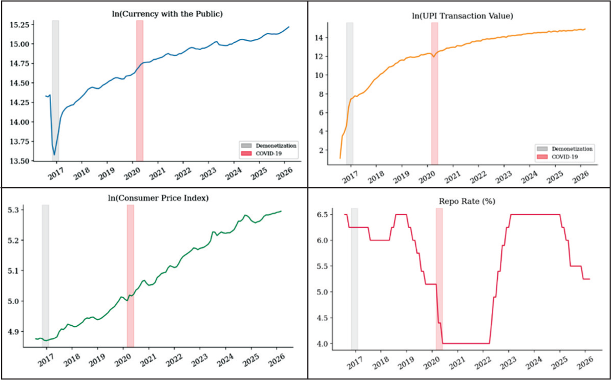
Figure 1 plots all four log-transformed variables and the repo rate over the sample period, with shading marking the demonetization (November 2016 to February 2017) and COVID-19 (March–June 2020) windows. The sharp contraction in lnCwP during demonetization, the subsequent recovery and the surge during the COVID-19 lockdown are clearly visible, confirming the importance of explicit structural break controls in the estimation.

Figure 1.

Time Series Plots of ln(CwP), ln(UPI), ln(CPI) and Repo Rate, August 2016 to March 2026.

Treatment of Structural Breaks

The sample contains two episodes that constitute structural breaks in the CwP series and, if left unaddressed, would bias the long-run coefficient estimates and potentially generate spurious cointegration results. The first is the demonetization of 8 November 2016, which caused an abrupt and historically unprecedented contraction in CwP as holders of the demonetized notes deposited them in banks. The second is the onset of the COVID-19 pandemic and the associated national lockdown in March 2020, which triggered a sharp increase in precautionary cash demand unrelated to any change in the attractiveness of digital payments.

Both episodes are controlled for through additive dummy variables. The demonetization dummy (DEMO) equals one for November 2016 through February 2017, covering the acute disruption from the withdrawal announcement through the initial remonetization period, and zero elsewhere. The COVID-19 dummy (COVID) equals one for March 2020 through June 2020, covering the national lockdown period during which precautionary cash hoarding was most intense, and zero for elsewhere. These dummies enter the model as short-run additive terms, absorbing transitory shock effects without altering the long-run equilibrium relationship among the variables. Parameter stability over the remainder of the sample is confirmed through CUSUM and CUSUMSQ tests.

Model Specification

Following the transaction-cost inventory framework of Whitesell (1989) and Alvarez and Lippi (2009), and the standard nominal money-demand specification of Goldfeld et al. (1973), the long-run equilibrium demand for physical currency can be derived as follows. The representative agent minimizes the total cost of conducting a given volume of transactions. The cost of holding physical currency includes the inflation tax on nominal balances and the opportunity cost relative to bank deposits. The cost of using UPI includes fixed access costs that are inversely reflected in observed adoption: a higher UPI transaction value is the revealed outcome of agents finding digital payment cost-minimizing for an expanding share of transactions.

This minimization yields:

\ln C w P_{t} = α_{0} + α_{1} \ln C P I_{t} + α_{2} R E P O_{t} + α_{3} \ln U P I_{t} + ε_{t} ​,

(1)

where lnCwP_t is the log of CwP; α₁> 0 because a higher price level raises the nominal demand for physical currency; α₂ < 0 because a higher opportunity cost reduces the demand for non-interest-bearing cash; α₃ is theoretically ambiguous in sign: The substitution effect predicts a negative coefficient, while the income effect operating through expanding aggregate transaction volumes predicts a positive coefficient; the net long-run sign is an empirical matter addressed by the NARDL asymmetric decomposition; and ε_t is the error term. The asymmetric extension of this model posits that α₃ is not a single symmetric coefficient but rather a pair of long-run effects, one governing the response of CwP to positive changes in lnUPI_t and another to negative changes. The transaction-cost framework of Alvarez and Lippi (2009) predicts that the two coefficients will differ in magnitude, with the response to sustained UPI contractions exceeding in absolute value the response to equivalent expansions, a prediction that the Wald asymmetry test directly evaluates.

Unit Root Testing

The NARDL bounds testing procedure requires that no variable in the model be integrated of order two, I(2), since the asymptotic critical values tabulated by Pesaran et al. (2001) are valid only for variables that are I(0) or I(1), or a mixture of the two. To establish the order of integration of each series, three complementary tests are applied: the augmented Dickey–Fuller (ADF) test (Dickey & Fuller, 1981), the Phillips–Perron (PP) test (Phillips & Perron, 1988) and the Kwiatkowski–Phillips–Schmidt–Shin (KPSS) test (Kwiatkowski et al., 1992). The ADF and PP share the unit-root null hypothesis but differ in how they correct for serial correlation: the ADF uses parametric lagged differences, and the PP uses a nonparametric Newey–West correction. Their joint use reduces the risk of incorrect inference from the well-known low-power problem of each method used individually. The KPSS reverses the null, testing stationarity against the unit root alternative, providing a further check. Each variable is tested at levels and first differences, with AIC-selected lag lengths for the ADF and a Newey–West procedure for the KPSS bandwidth.

Given the structural breaks in lnCwP_t, the Zivot and Andrews (2002) test is applied as a supplementary check. This test endogenously identifies the most likely breakpoint and determines whether lnCwP_t is stationary around that breakpoint or genuinely I(1). It guards against the well-documented tendency of standard tests to over-reject the stationarity null in the presence of level shifts, which would erroneously classify a break-stationary process as I(1) and invalidate the bounds testing framework.

The NARDL Model: Decomposition and Estimation

The NARDL model decomposes lnUPI into its positive and negative partial sums. Let ΔlnUPI_t denote the first difference of the log UPI series. Then,

\ln U P I_{t}^{+} = \sum_{i = 1}^{t} \max (Δ \ln U P I_{i}, ​ ​ 0),

(2)

\ln U P I_{t}^{-} = \sum_{i = 1}^{t} \min (Δ \ln U P I_{i}, 0) ​,

(3)

where lnUPl⁺_t is the cumulative sum of positive changes in log UPI transaction value, capturing periods of accelerating digital adoption, and lnUPl^–_t is the cumulative sum of negative changes, capturing contractions or slowdowns. By construction lnUPI_t = lnUPI₀ + lnUPl⁺_t + lnUPl^–_t, so the decomposition is exhaustive and preserves all information in the original series. These two partial sum series replace lnUPI in the regression, allowing their effects on lnCwP to be estimated independently. The NARDL model in unrestricted error-correction form, augmented with the structural break dummies, is

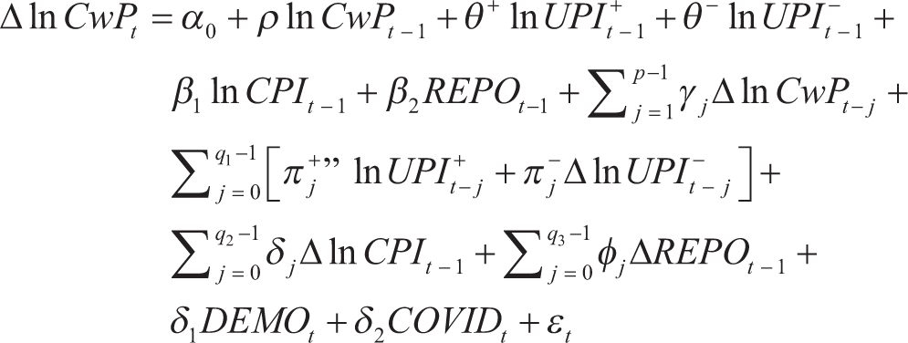
\begin{array}{l} Δ \ln C w P_{t} = α_{0} + ρ \ln C w P_{t - 1} + θ^{+} \ln U P I_{t - 1}^{+} + θ^{-} \ln U P I_{t - 1}^{-} + \\ β_{1} \ln C P I_{t - 1} + β_{2} R E P O_{t - 1} + \sum_{j = 1}^{p - 1} γ_{j} Δ \ln C w P_{t - j} + \\ \sum_{j = 0}^{q_{1} - 1} [π_{j}^{+} Δ \ln U P I_{t - j}^{+} + π_{j}^{-} Δ \ln U P I_{t - j}^{-}] + \\ \sum_{j = 0}^{q_{2} - 1} δ_{j} Δ \ln C P I_{t - 1} + \sum_{j = 0}^{q_{3} - 1} ϕ_{j} Δ R E P O_{t - 1} + \\ δ_{1} D E M O_{t} + δ_{2} C O V I D_{t} + ε_{t} \end{array}

(4)

In equation (4), r is the error-correction coefficient, which must be negative and statistically significant for cointegration to hold; its absolute value measures the fraction of the long-run disequilibrium corrected each month. The parameters t + and t – are the level coefficients on lnUPI⁺ and lnUPI⁺, respectively. The normalized long-run effects are recovered as L⁺ = $- \frac{θ^{+}}{ρ}$ and L⁻ = $- \frac{θ^{-}}{ρ}$ , representing the long-run impact on lnCwP of a one-unit sustained positive or negative change in lnUPI. Similarly, the normalized long-run effects of ln CPI and REPO are $- \frac{β_{1}}{ρ}$ and $- \frac{β_{2}}{ρ}$ . The short-run dynamic coefficients γ_j, π⁺_j, π^–_j, δ_j and φ_j govern the adjustment path towards equilibrium. The structural break dummies enter as short-run additive terms, absorbing the transitory shock effects without altering the long-run relationship. Lag orders p, q₁, q₂ and q₃ are selected jointly by the Akaike Information Criterion with a maximum of three lags, verified to produce serially uncorrelated residuals. All standard errors are heteroscedasticity-consistent (HC1).

Bounds Test for Asymmetric Cointegration

The existence of a long-run level relationship is tested using the bounds F-test of Pesaran et al. (2001), adapted for the NARDL context by Shin et al. (2014). The null hypothesis is $H 0_{0} : ρ = θ^{+} = θ^{-} = β_{1}$ = $β_{2}$ = 0, representing the absence of any long-run relationship among lnCwP, lnUPI⁺, lnUPI^–, lnCPI and REPO. The F-statistic is compared against the Case III critical bounds from Pesaran et al. (2001), Table CI(iii), with k = 4 regressors, corresponding to an unrestricted intercept and no deterministic trend. If the F-statistic exceeds the upper I(1) bound, cointegration is confirmed regardless of the actual integration orders of the individual regressors. If it falls below the lower I(0) bound, cointegration is rejected. If it lies between the two bounds, the result is inconclusive, and the unit root results must be relied upon to proceed.

Tests for Long-run and Short-run Asymmetry

The NARDL framework permits formal statistical testing of whether the long-run and short-run effects of UPI on CwP are symmetric or asymmetric. Long-run asymmetry is assessed through a Wald test of H0₀: L⁺ = L^–, equivalently H0₀: θ ⁺ = θ ^–, against the two-sided alternative that the normalized long-run coefficients differ. Rejection of this null implies that the long-run response of CwP to a sustained UPI expansion differs in magnitude from the response to an equivalent sustained contraction. Short-run additive asymmetry is tested through a Wald test of H₀: $\sum π_{j}^{+} = \sum π_{j}^{-}$ , that is, whether the cumulative short-run impact of UPI growth equals the cumulative impact of UPI decline. Together, these two tests determine whether the NARDL specification is statistically warranted relative to the symmetric linear ARDL. Rejection of the long-run null is the more economically significant result because it speaks directly to the structural cash–digital relationship, whereas short-run asymmetry may reflect transitory adjustment dynamics.

Diagnostic and Stability Tests

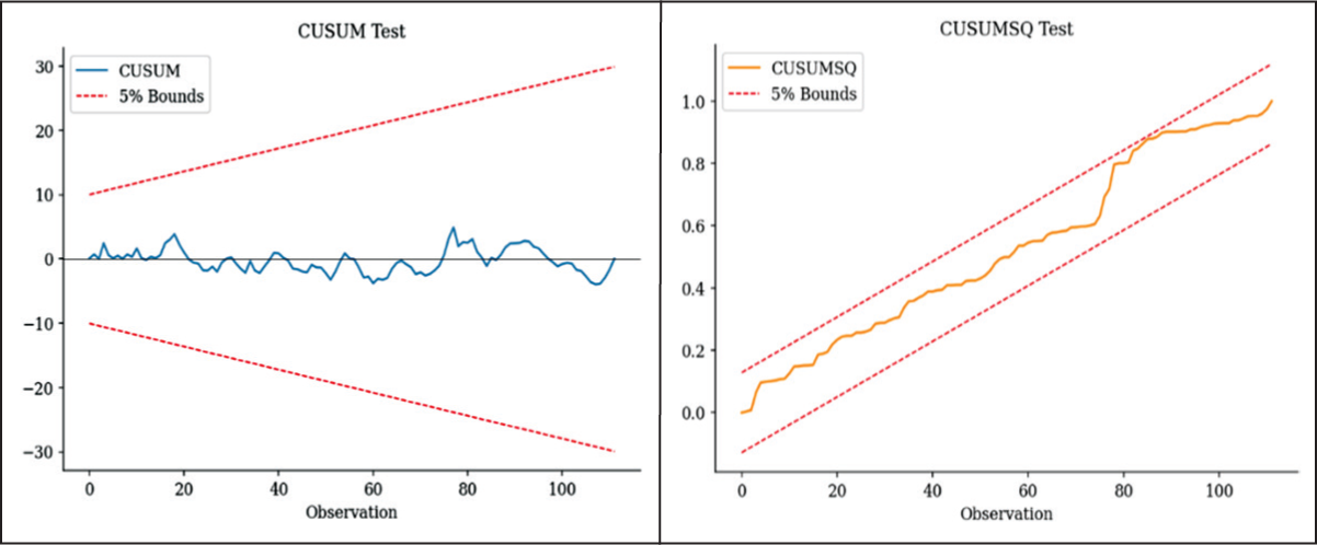
The reliability of the NARDL estimates is verified through four diagnostic tests. Serial correlation in the residuals is examined using the Breusch-Godfrey Lagrange multiplier test (Breusch, 1978; Godfrey, 1978) up to lag order two, under the null of no serial correlation. Heteroscedasticity is examined using the Breusch–Pagan–Godfrey test (Breusch & Pagan, 1979) under the null of homoscedastic errors. The normality of residuals is evaluated using the Jarque–Bera test (Jarque & Bera, 1980). Parameter stability is assessed through the CUSUM and CUSUMSQ tests of Brown et al. (1975). Because the structural break dummies are explicitly included in the model, the CUSUM and CUSUMSQ statistics are expected to remain within the 5% critical bounds throughout the sample, confirming that the dummy variable approach adequately captures the demonetization and COVID-19 episodes.

Results and Discussion

Descriptive Statistics

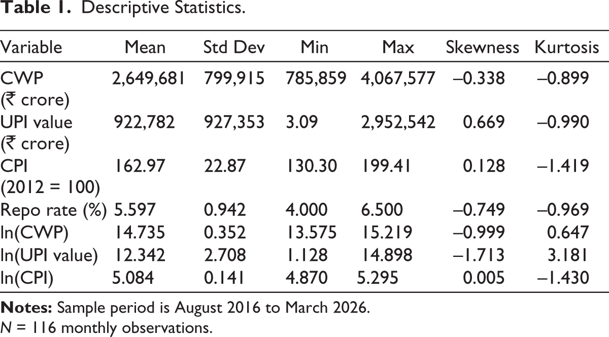
Table 1 presents descriptive statistics for both the raw and log-transformed variables. Over the sample period, CwP averaged ₹26.5 lakh crore with a standard deviation of ₹8.0 lakh crore, reflecting the persistent upward trend that defines the Indian cash paradox. UPI transaction value grew from near zero at the start of the sample to ₹29.5 lakh crore by March 2026, with a mean of ₹9.2 lakh crore and a standard deviation that nearly matches the mean, indicative of explosive non-linear growth. CPI averaged 162.97 on the 2012 base, rising steadily from 131.1 in August 2016 to 199.4 by March 2026, consistent with the RBI’s inflation targeting experience over this period. The repo rate averaged 5.60%, ranging from a post-pandemic low of 4.00% to a high of 6.50% in 2016 and again during the monetary policy tightening phase of 2022 to 2023.

Table 1.

Descriptive Statistics.

Variable	Mean	Std Dev	Min	Max	Skewness	Kurtosis
CWP (₹ crore)	2,649,681	799,915	785,859	4,067,577	–0.338	–0.899
UPI value (₹ crore)	922,782	927,353	3.09	2,952,542	0.669	–0.990
CPI (2012 = 100)	162.97	22.87	130.30	199.41	0.128	–1.419
Repo rate (%)	5.597	0.942	4.000	6.500	–0.749	–0.969
ln(CWP)	14.735	0.352	13.575	15.219	–0.999	0.647
ln(UPI value)	12.342	2.708	1.128	14.898	–1.713	3.181
ln(CPI)	5.084	0.141	4.870	5.295	0.005	–1.430

Notes: Sample period is August 2016 to March 2026.

N = 116 monthly observations.

The log-transformed series reveals important distributional features. The lnCwP series displays mild negative skewness (–0.999), reflecting the sharp but temporary decline during demonetization in late 2016. The lnUPI series exhibits strong negative skewness (–1.713) and excess kurtosis (3.181), reflecting the very low values at the sample start when UPI was in its infancy, and the explosive acceleration thereafter. These distributional characteristics confirm that the raw level relationships among the variables are unlikely to be well characterized by linear symmetric models and reinforce the rationale for the NARDL approach.

Unit Root Test Results

Table 2 reports the ADF, PP and KPSS unit root test results. The ADF and PP tests yield broadly consistent evidence. Both lnCwP and lnUPI are stationary in levels under both ADF (p = .0001 and p = .0011, respectively) and PP (p = .045 and p < .001), classifying them as I(0). By contrast, lnCPI and REPO are non-stationary in levels but stationary in first differences under both tests, classifying them as I(1). The KPSS test corroborates this mixed integration picture: the stationarity null is rejected in levels for all four series and fails to be rejected in first differences for lnCwP, lnCPI and REPO, though lnUPI remains borderline. This mixed I(0)/I(1) outcome is precisely the scenario for which the ARDL bounds testing approach is designed. The only binding constraint is the absence of I(2) variables, which the first-difference results confirm across all series, validating the application of the NARDL bounds testing procedure. The borderline KPSS result for ln(UPI) does not affect this conclusion since the bounds test critical values remain valid for any combination of I(0) and I(1) regressors.

Table 2.

Unit Root Test Results.

Variable	ADF Level	ADF First Diff	PP Level	PP First Diff	KPSS Level	KPSS First Diff	Order
ln(CWP)	–5.307***	–3.364**	–3.452**	–8.400***	0.359**	0.041	I(0)
ln(UPI)	–4.572***	–3.014**	–8.823***	–10.289***	0.396**	0.919***	I(0)/I(1)
ln(CPI)	–1.188	–6.535***	–2.437	–7.380***	0.199**	0.090	I(1)
REPO	–1.773	–3.872***	–1.729	–11.730***	0.271**	0.176	I(1)

Notes: ADF and PP include constant and trend in levels, constant only in first differences.

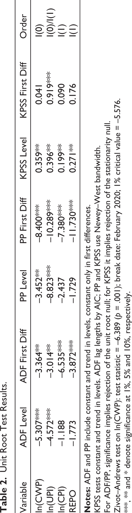
KPSS tests constant and trend in levels. ADF lag lengths by AIC; PP and KPSS use Newey–West bandwidth.

For ADF/PP, significance implies rejection of the unit root null; for KPSS it implies rejection of the stationarity null.

Zivot–Andrews test on ln(CWP): test statistic = –6.389 (p = .001); break date: February 2020; 1% critical value = –5.576.

***, ** and * denote significance at 1%, 5% and 10%, respectively.

The Zivot–Andrews test applied to lnCwP yields a test statistic of –6.39, which exceeds the 1% critical value of –5.58 in absolute value, rejecting the unit root null at the 1% level. The endogenously identified break date is February 2020, 1 month before the formal national lockdown of March 2020, consistent with the anticipatory precautionary cash accumulation that began as COVID-19 uncertainty spread globally in early 2020. This pre-lockdown break date is economically plausible and does not conflict with the COVID-19 dummy variable, which is set to 1 from March 2020 onwards to capture the acute lockdown phase.

Partial Sum Decomposition and NARDL Lag Selection

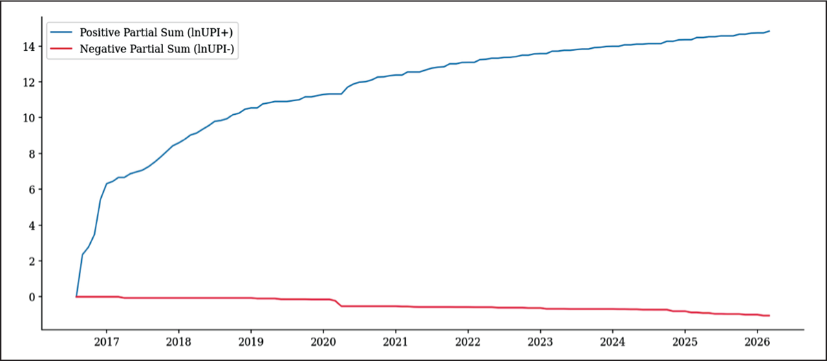
Figure 2 plots the positive and negative partial sums of lnUPI over the sample period. The positive partial sum (lnUPI⁺) increases monotonically and steeply from zero at the start of the sample, reflecting the near-uninterrupted growth in UPI transaction value throughout, and reaches a cumulative value of approximately 14.83 log points by March 2026. The negative partial sum (lnUPI^–) is comparatively small in absolute terms, ranging between 0 and –1.06 across the entire sample. This stark asymmetry in the scale of the two partial sums is itself an important preliminary finding: negative UPI shocks have been infrequent and modest in magnitude throughout the sample, while positive shocks have been the dominant feature. This asymmetry in the input data lends the formal Wald asymmetry tests economic as well as statistical significance. The AIC-based lag selection procedure identifies the optimal NARDL specification as NARDL(3,1,3,1), yielding a minimum AIC of –707.76 with serially uncorrelated residuals.

Figure 2.

Positive and Negative Partial Sums of ln(UPI), August 2016 to March 2026.

Bounds Test for Asymmetric Cointegration

Table 3 reports the bounds test results. The F-statistic for the joint null of no level relationship ( $H 0_{0} : ρ = θ^{+} = θ^{-} = β_{1}$ = $β_{2}$ = 0) is 7.507. This exceeds the Pesaran et al. (2001) upper I(1) critical bound of 5.61 at the 1% significance level for Case III with k = 4 regressors, providing strong evidence of a long-run cointegrating relationship among lnCwP, lnUPI ⁺, lnUPI^–, lnCPI and REPO, regardless of the precise integration orders of the individual series. The null of no cointegration is strongly rejected, establishing the foundation for interpreting the long-run NARDL coefficients.

Table 3.

Bounds Test for Asymmetric Cointegration.

	F-Statistic	I(0) Lower Bound	I(1) Upper Bound	Decision
Test statistic (k = 4)	7.507***			Cointegrated
1% critical values		4.29	5.61
5% critical values		3.23	4.35
10% critical values		2.72	3.77

Notes: Critical values from Pesaran et al. (2001), Table CI(iii), Case III (unrestricted intercept, no trend), k = 4.

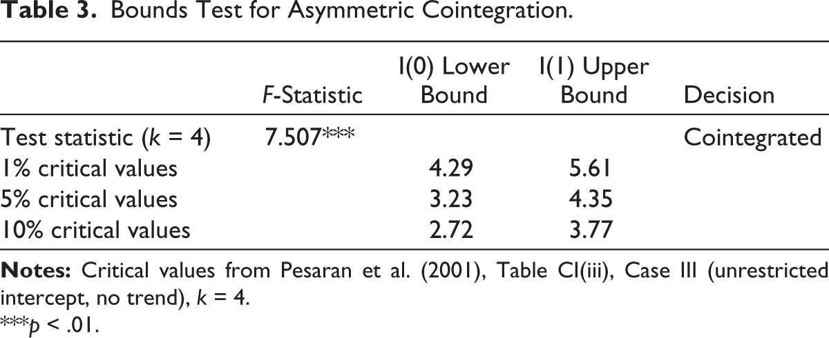
***p < .01.

Long-run Coefficients and Asymmetry

Table 4 presents the normalized long-run coefficients and the Wald asymmetry test results. The error-correction coefficient r = 0.374 is significant at the 1% level (p < .001), confirming that approximately 37.4% of any deviation from long-run equilibrium is corrected within a single month. This relatively brisk adjustment speed is consistent with the liquidity of cash holdings relative to other asset classes, and the negative, significant r confirms that the cointegrating vector is stable and that the system returns to equilibrium following any shock.

Table 4.

NARDL Long-run Coefficient Estimates, Error Correction and Asymmetry Tests.

Variable	Level Coeff.	Std Err (HC1)	z-stat	p Value	Norm. LR Coeff.
lnUPI⁺ (positive shocks)	0.031	0.007	4.739	.000***	L⁺ = +0.083
lnUPI^– (negative shocks)	–0.066	0.024	–2.758	.006***	L^– = –0.178
ln(CPI)	0.147	0.063	2.351	.019**	L_CPI = +0.394
REPO	–0.004	0.002	–1.600	.110	L_REPO = –0.010
Error correction (r)	–0.374	0.065	–5.709	.000***
Wald test: long-run $H 0_{0} : L^{+} = L^{-}$	F = 11.629			.001***	Reject H₀
Wald test: short-run $H 0_{0} : \sum π_{j}^{+} = \sum π_{j}^{-}$	F = 2.339			.130	Fail to reject

Notes: Level coefficients from NARDL(3,1,3,1) with HC1 robust standard errors.

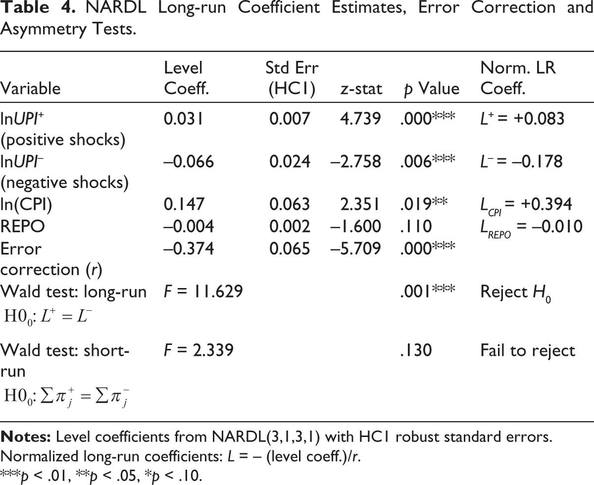
Normalized long-run coefficients: L = – (level coeff.)/r.

***p < .01, **p < .05, *p < .10.

The normalized long-run coefficient on positive UPI shocks (L⁺) is +0.083 (p < .001). Within the transaction-cost framework developed in the ‘Literature Review’ section, this positive sign is theoretically consistent with the Baumol (1952) income elasticity of physical currency demand. Whitesell (1989) and Alvarez and Lippi (2009) both recognize that the equilibrium stock of physical currency depends not only on the relative cost of payment instruments but also on the volume of transactions agents need to finance. Periods of rapid UPI expansion in the sample coincide with phases of broad economic growth, rising incomes and expanding aggregate transaction volumes, all of which independently raise the transactions demand for physical currency. The substitution effect of UPI adoption, which would reduce CwP, is therefore dominated by the income-driven transactions demand effect in the long run. Households and firms that adopt UPI appear to use it for an incremental set of transactions rather than displacing existing cash-financed ones, consistent with Jobst and Stix (2017), who document the same payment instrument complementarity in European data. India’s large informal sector, where physical currency remains the default medium of exchange, further means that aggregate CwP remains responsive to income even as the formal digital payment economy expands. This is further confirmed by the positive and significant contemporaneous short-run coefficient on ΔlnUPI⁺: months of high UPI activity are also months of elevated income and spending, raising demand for physical currency alongside digital payment demand.

The normalized long-run coefficient on negative UPI shocks (L⁻) is –0.178, significant at the 1% level (p = .006). This result directly confirms the Alvarez and Lippi (2009) prediction that precautionary currency accumulation during digital payment contractions structurally exceeds the marginal reduction during normal expansion. The ratio |L⁻ |/|L⁺ | = 0.178/0.083 = 2.1 quantifies this asymmetry: a sustained contraction in UPI activity has more than twice the long-run impact on CwP as an equivalent expansion. The Wald test for long-run asymmetry, with F = 11.629 (p = .001), is therefore not merely a statistical test of coefficient equality but a formal test of the structural prediction generated by the transaction-cost inventory model. Its decisive rejection of the null confirms that the asymmetric NARDL specification captures a genuine structural feature of the physical currency–digital payment relationship in India, consistent with Keynes’s (1936) precautionary motive operating asymmetrically across states of digital payment availability.

The normalized long-run coefficient on lnCPI is +0.394, significant at the 5% level (p = .019), indicating that a 1% increase in the price level raises long-run CwP by approximately 0.39%. This is consistent with the standard nominal money demand framework: higher prices raise the nominal value of transactions and, in turn, the demand for nominal cash balances. The coefficient below unity is consistent with standard money demand estimates in the literature and may also partially reflect the growing share of digital transactions absorbing nominal spending that would otherwise have been cash-financed. The long-run coefficient on REPO is –0.010, carrying the theoretically expected negative sign but insignificant at conventional levels (p = .110). Within the Whitesell (1989) transaction-cost framework, this result is consistent with the theoretical prediction that the relevant cost driving physical currency demand in India is the fixed cost of accessing and holding physical notes relative to digital alternatives, not the interest rate differential between cash and bank deposits. The population holding the largest share of physical currency in India consists predominantly of informal sector workers, rural households and the financially excluded, for whom the opportunity cost of cash relative to bank deposits is not a salient consideration because they have limited access to interest-bearing alternatives in the first place. Their physical currency demand is driven by access constraints, not by the policy rate.

Short-run Dynamics and Error Correction

Table 5 presents the full short-run ECM results from the NARDL(3,1,3,1) model. The model fits the data well, with an R² of 0.919 and an adjusted R² of 0.905, explaining more than 90% of the monthly variation in the change in lnCwP. The overall F-statistic of 510.0 (p < .001) confirms strong joint significance.

Table 5.

Short-run ECM Results from NARDL(3,1,3,1).

Variable	Coefficient	Std Err (HC1)	z-Stat	p Value
Constant	4.392	0.871	5.042	.000***
ΔlnCwp_t_{– 1}	0.324	0.041	7.827	.000***
ΔlnCwp_t_{– 2}	–0.048	0.029	–1.674	.094*
ΔlnCwp_t_{– 3}	0.002	0.030	0.059	.953
ΔlnUPI⁺_t	0.032	0.015	2.094	.036**
ΔlnUPI^–_t	–0.025	0.029	–0.852	.394
ΔlnCPI_t	0.113	0.155	0.726	.468
ΔlnCPI_t_{– 1}	–0.286	0.143	–1.994	.046**
ΔlnCPI_t_{– 2}	–0.699	0.143	–4.905	.000***
ΔREPO_t	0.010	0.005	1.781	.075*
DEMO	–0.057	0.031	–1.810	.070*
COVID	0.017	0.006	2.922	.003***
R ²	0.919
Adj. R²	0.905
F-statistic	510.0			0.000***
Observations	112

Notes: Dependent variable is delta ln(CWP).

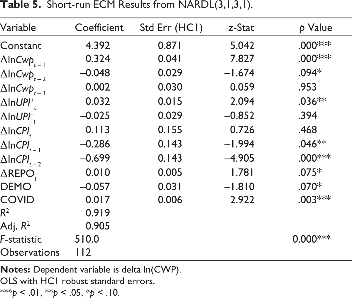
OLS with HC1 robust standard errors.

***p < .01, **p < .05, *p < .10.

Among the short-run UPI coefficients, the contemporaneous impact of positive UPI shocks (ΔlnUPI⁺_t = 0.032, p = .036) is positive and statistically significant. As noted in the ‘Long-run Coefficients and Asymmetry’ section, this reflects the income effect on cash demand dominating the substitution effect in the immediate month following a UPI transaction increase: months of high UPI activity also tend to be months of elevated economic activity and aggregate spending, which raise cash demand. The contemporaneous negative UPI shock coefficient (ΔlnUPI^–_t = –0.025) carries the theoretically expected negative sign but is not statistically significant (p = .394), confirming the absence of a statistically distinguishable short-run asymmetry, consistent with the Wald test result in Table 4.

Among the lagged dependent variable terms, the first lag ΔlnCwP (t – 1) carries a large and highly significant coefficient of 0.324 (p < .001), indicating strong positive autocorrelation in monthly cash changes and reflecting the gradual and persistent nature of cash holding adjustments. The price level dynamics reveal an important pattern: while the contemporaneous ΔlnCPI_t is insignificant (p = .468), the first lag ΔlnCPI_t_{– 1} (coefficient = –0.286, p = .046) and second lag ΔlnCPI_t_{– 2} (coefficient = –0.699, p < .001) are negative and significant. This pattern of negative lagged CPI coefficients alongside a positive long-run CPI coefficient reflects the delayed pass-through of price-level changes into nominal cash holdings, a feature commonly documented in emerging-market money-demand studies, where cash adjustment to inflation is gradual rather than immediate.

The DEMO carries a coefficient of –0.057 (p = .070), marginally significant at the 10% level, confirming the expected short-run contraction in CwP during the November 2016 to February 2017 window. The COVID-19 dummy (COVID) is positive and highly significant (0.017, p = .003), capturing the sharp precautionary cash accumulation during the March to June 2020 lockdown period, consistent with the RBI’s documentation of anomalously high CwP growth during that period (RBI, 2021).

Diagnostic Tests and Parameter Stability

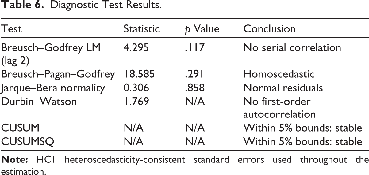
Table 6 presents the diagnostic test results. The Breusch–Godfrey LM test for serial correlation up to lag order two yields a statistic of 4.295 with a p value of 0.117, failing to reject the null of no serial correlation. The Breusch–Pagan–Godfrey test yields a statistic of 18.585 and a p value of 0.291, confirming homoscedasticity. The Jarque–Bera test yields a statistic of 0.306 with a p value of 0.858, indicating that the residuals are consistent with normality. The Durbin–Watson statistic of 1.769 provides further support for the absence of first-order autocorrelation. Together, these results confirm that the model is well-specified and that inference based on HC1 robust standard errors is valid.

Table 6.

Diagnostic Test Results.

Test	Statistic	p Value	Conclusion
Breusch–Godfrey LM (lag 2)	4.295	.117	No serial correlation
Breusch–Pagan–Godfrey	18.585	.291	Homoscedastic
Jarque–Bera normality	0.306	.858	Normal residuals
Durbin–Watson	1.769	N/A	No first-order autocorrelation
CUSUM	N/A	N/A	Within 5% bounds: stable
CUSUMSQ	N/A	N/A	Within 5% bounds: stable

Note: HC1 heteroscedasticity-consistent standard errors used throughout the estimation.

The CUSUM and CUSUMSQ test plots in Figure 3 show that both statistics remain within the 5% critical bounds throughout the estimation period. This confirms parameter stability across the full sample and validates the dummy variable treatment of the structural breaks. Had the demonetization and COVID-19 episodes gone unaddressed, the CUSUM statistic would likely have exceeded the bounds in late 2016 and again in early 2020.

Figure 3.

CUSUM and CUSUMSQ Parameter Stability Tests for the NARDL(3,1,3,1) Model.

Dynamic Multipliers

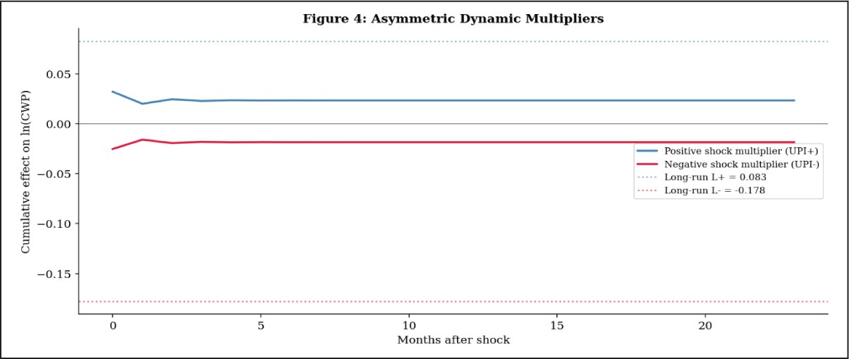
Figure 4 presents the asymmetric dynamic multipliers, which trace the cumulative effect on lnCwP of a unit positive or negative shock to lnUPI over a 24-month horizon following the shock. The positive shock multiplier (lnUPI⁺) converges from above towards its long-run value of L⁺ = +0.083, while the negative shock multiplier (lnUPI^–) converges from below towards L^– = –0.178. The speed of convergence is governed by the error-correction coefficient of –0.374, implying that the bulk of the long-run adjustment is completed within 5 to 6 months of the shock. The divergence between the two multiplier paths is visually apparent from the first month onwards and continues to widen until convergence, providing a graphical counterpart to the Wald test result that formally confirms the presence of long-run asymmetry. The multiplier plots also make plain the economic significance of the asymmetry: negative shocks to UPI adoption have more than twice the long-run impact on CwP than positive shocks of equivalent magnitude, underlining the disproportionate role of downside digital payment disruptions in driving precautionary cash accumulation.

Figure 4.

Asymmetric Dynamic Multipliers of Positive and Negative UPI Shocks on ln(CwP) over a 24-Month Horizon.

Conclusion

India’s experience with digital payments over the past decade reveals a fundamental limitation of the cash substitution hypothesis: in an economy where income growth, informality and financial exclusion independently sustain the demand for physical currency, the proliferation of digital payment instruments does not necessarily reduce the stock of notes and coins in public hands. The asymmetric NARDL evidence establishes that UPI and physical currency have coexisted as structural complements rather than substitutes. Rising UPI adoption coincides with economic expansion, which raises demand for cash transactions, while contractions in digital payment activity trigger precautionary currency accumulation that is disproportionately large relative to any substitution in normal times. Physical currency in India remains the instrument of last resort for a substantial share of the population, and this role is not diminishing as digital penetration increases.

The theoretical framework developed in this article grounds these findings in the transaction-cost inventory tradition of Whitesell (1989) and Alvarez and Lippi (2009). In this framework, the equilibrium stock of physical currency reflects agents’ cost minimization over the fixed costs of accessing cash and the fixed costs of using digital payment instruments. UPI has reduced the latter through the Jio-era collapse in mobile data costs and the elimination of transaction fees, but it has not eliminated the former. The fixed cost of accessing physical currency, including proximity to banking infrastructure and the reliability of digital alternatives, remains salient for a large share of India’s population. More importantly, the Alvarez and Lippi (2009) model predicts that when digital payment availability contracts, agents respond by holding more cash than the symmetric substitution relationship would imply, because the option value of physical currency as a fallback rises precisely when digital infrastructure is unreliable. The empirical asymmetry confirmed here is therefore not a statistical anomaly but the predicted outcome of rational inventory management under conditions of imperfect and asymmetrically distributed digital access. Policy prescriptions that ignore this theoretical structure risk misdiagnosing the cash paradox as a transitional problem amenable to digital push strategies, when it is in fact a structural equilibrium outcome.

The most consequential implication of these findings is for how the RBI conceptualizes the relationship between financial digitalization and currency management. The assumption, implicit in much of the policy discourse on India’s cashless economy agenda, that rising UPI adoption will progressively compress physical currency demand and ease the operational burden of currency issuance, is not supported by the evidence. Income growth sustains currency demand regardless of the pace of digital adoption, and the population segments that hold the largest share of physical currency, namely rural households, informal sector workers and the financially excluded, are structurally insulated from the substitution effect. Currency management planning that treats UPI growth as a leading indicator of declining CwP will systematically underestimate future currency requirements, with supply shortfalls falling hardest on those least able to absorb them. The insignificant long-run repo rate coefficient reported in Table 4 reinforces this point: conventional monetary policy has limited direct traction on physical currency demand because the population holding the bulk of India’s physical currency has restricted access to interest-bearing alternatives and is therefore insensitive to changes in the policy rate.

The precautionary asymmetry documented here reframes the question of payment system resilience as a monetary concern. When digital payment infrastructure is disrupted, whether by technical failure, cybersecurity incidents or a loss of public confidence, the resulting surge in physical currency demand is structurally larger and faster than any reduction achieved during normal periods of UPI expansion. The long-run coefficient L = –0.178 implies that a sustained 10% contraction in UPI transaction value raises long-run CwP by approximately 1.78%, equivalent to ₹700 to 800 billion in additional physical currency demand at current levels, with the bulk of adjustment completing within 5 to 6 months, given the error-correction speed of 37.4% per month. The central bank cannot treat the stability of the digital payments ecosystem as external to its currency management mandate. Investing in the resilience of UPI infrastructure, maintaining adequate physical currency buffers and ensuring that contingency arrangements for payment system failures are clearly communicated to the public are implications that flow directly from the asymmetric structure of the cash–digital relationship documented here. Structural interventions that reduce the access cost of digital payment instruments, including rural broadband connectivity, UPI onboarding for informal merchants and digital literacy programmes, are likely to be more effective levers for reducing aggregate CwP than changes in the policy repo rate because they address the fixed access cost differential that the transaction-cost framework identifies as the primary determinant of equilibrium physical currency demand.

Several limitations of this study suggest directions for future work. The aggregate framework cannot identify which population segments or regions drive the cash paradox; panel data at the household or state level would allow more targeted analysis. Whether the asymmetric relationship has weakened as UPI has matured could be examined with a time-varying parameter approach. The substitution potential of the RBI’s central bank digital currency remains empirically untested, given its limited circulation during the sample period. Extending the analysis to economies with comparable instant payment systems, such as Brazil’s PIX or Singapore’s PayNow, would help determine whether structural complementarity between digital payments and physical currency is a general feature of large developing economies or a condition specific to India.

Footnotes

Data Availability Statement

The data that support the findings of this study are available upon request. These data were derived from the following public-domain resources: RBI DBIE and NPCI.

Declaration of Conflicting Interests

The author declared no potential conflicts of interest with respect to the research, authorship and/or publication of this article.

Funding

The author received no financial support for the research, authorship and/or publication of this article.

References

Agarwal

, Ghosh

, Li

, & Ruan

(2024). Digital payments and consumption: Evidence from the 2016 demonetization in India. The Review of Financial Studies, 37(8), 2550–2585.

Akber

, Gupta

, & Paltasingh

K. R.

(2020). The crowding-in/out debate in investments in India: Fresh evidence from NARDL application. South Asian Journal of Macroeconomics and Public Finance, 9(2), 167–189.

Alvarez

, & Lippi

(2009). Financial innovation and the transactions demand for cash. Econometrica, 77(2), 363–402.

Amromin

, & Chakravorti

(2009). Whither loose change? The diminishing demand for small-denomination currency. Journal of Money, Credit and Banking, 41(2–3), 315–335.

Baumol

W. J.

(1952). The transactions demand for cash: An inventory theoretic approach. The Quarterly Journal of Economics, 66(4), 545–556.

Breusch

T. S.

(1978). Testing for autocorrelation in dynamic linear models. Australian Economic Papers, 17(31), 334–355.

Breusch

T. S.

, & Pagan

A. R.

(1979). A simple test for heteroscedasticity and random coefficient variation. Econometrica, 47(5), 1287–1294.

Brown

R. L.

, Durbin

, & Evans

J. M.

(1975). Techniques for testing the constancy of regression relationships over time. Journal of the Royal Statistical Society: Series B (Methodological), 37(2), 149–163.

Chaudhry

A., Chandni

, & Dudeja

(2026). Investigating asymmetric effects of electronic payment on money supply for India using non-linear ARDL model. Millennial Asia, 17(1), 136–160.

10.

Dickey

D. A.

, & Fuller

W. A.

(1981). Likelihood ratio statistics for autoregressive time series with a unit root. Econometrica, 49(4), 1057–1072.

11.

Fujiki

, & Tanaka

(2010). Currency demand, new technology and the adoption of electronic money: Evidence using individual household data. Science and Technology, 125, 5–8.

12.

Godfrey

L. G.

(1978). Testing against general autoregressive and moving average error models when the regressors include lagged dependent variables. Econometrica, 46(6), 1293–1301.

13.

Goldfeld

S. M.

, Duesenberry

, & Poole

(1973). The demand for money revisited. Brookings Papers on Economic Activity, 1973(3), 577–646.

14.

Jarque

C. M.

, & Bera

A. K.

(1980). Efficient tests for normality, homoscedasticity and serial independence of regression residuals. Economics Letters, 6(3), 255–259.

15.

Jobst

, & Stix

(2017). Doomed to disappear? The surprising return of cash across time and across countries (CEPR Discussion Paper No. DP12327). Centre for Economic Policy Research.

16.

Keynes

J. M.

(1936). The general theory of employment, interest and money. Macmillan.

17.

Kwiatkowski

, Phillips

P. C. B.

, Schmidt

, & Shin

(1992). Testing the null hypothesis of stationarity against the alternative of a unit root: How sure are we that economic time series have a unit root? Journal of Econometrics, 54(1–3), 159–178.

18.

National Payments Corporation of India (NPCI). (2026). UPI product statistics: Monthly transaction value and volume, August 2016 to March 2026. NPCI. https://www.npci.org.in/product/upi/product-statistics

19.

Ozili

P. K.

(2018). Impact of digital finance on financial inclusion and stability. Borsa Istanbul Review, 18(4), 329–340.

20.

Ozturk

, & Ullah

(2022). Does digital financial inclusion matter for economic growth and environmental sustainability in OBRI economies? An empirical analysis. Resources, Conservation and Recycling, 185, 106489.

21.

Pesaran

M. H.

, Shin

, & Smith

R. J.

(2001). Bounds testing approaches to the analysis of level relationships. Journal of Applied Econometrics, 16(3), 289–326.

22.

Phillips

P. C. B.

, & Perron

(1988). Testing for a unit root in time series regression. Biometrika, 75(2), 335–346.

23.

Reserve Bank of India (RBI). (2021). Annual report 2020–21. Reserve Bank of India.

24.

Reserve Bank of India (RBI). (2026). Database on the Indian Economy (DBIE): Currency with the public, policy repo rate, consumer price index (August 2016 to March 2026). https://data.rbi.org.in/DBIE

25.

Sharma

, Adil

M. H.

, Fatima

, & Mittal

(2024). Asymmetric effect of fiscal deficit on current account deficit: Evidence from India. Vision, 28(4), 480–493.

26.

Shin

, Yu

, & Greenwood-Nimmo

(2014). Modelling asymmetric cointegration and dynamic multipliers in a nonlinear ARDL framework. In Sickles

& Horrace

(Eds.), Festschrift in honor of Peter Schmidt (pp. 281–314). Springer.

27.

Singh

V. K.

, & Ghosh

(2021). Financial inclusion and economic growth in India amid demonetization: A case study based on panel cointegration and causality. Economic Analysis and Policy, 71, 674–693.

28.

Tobin

(1956). The interest-elasticity of transactions demand for cash. The Review of Economics and Statistics, 38(3), 241–247.

29.

Whitesell

W. C.

(1989). The demand for currency versus debitable accounts. Journal of Money, Credit and Banking, 21(2), 246–251.

30.

Zivot

, & Andrews

D. W. K.

(2002). Further evidence on the great crash, the oil-price shock, and the unit-root hypothesis. Journal of Business & Economic Statistics, 20(1), 25–44.