Quasi-Monte Carlo Approach to Asian Options Pricing

Abstract

Asian options is a contract which gives right to the holder to buy/sell the underlying asset for its average price over prescribed period and it has a lower unpredictability, hence exposing cheaper relative to their European counterparts. Asian options are commonly traded on currencies and commodity products which have low trade volumes. Therefore, the pricing of such options become one of the most interesting fields. Much research work has been done on the European and American options using various techniques like Black-Scholes, binomial tree, finite difference, Monte Carlo and Quasi-Monte Carlo model. But none of the studies compares and identified the best model for options pricing, particularly for Asian options pricing. This article aims to evaluate the effectiveness of existing models on Asian options pricing and to suggest a suitable model for forecasting Asian options prices. Findings of the study indicate that the Quasi-Monte Carlo technique is more superior to any other techniques due to its results with high precision and low standard deviation.

Keywords

Black Scholes derivatives options options pricing Monte Carlo simulation Quasi-Monte Carlo simulation model

Introduction

Derivatives are financial contracts, whose behaviour depends on the value of the underlying assets. The underlying value on which a derivative is based can be a traded asset, such as a stock, an index portfolio, a futures price, a commercial real estate, etc. Derivatives can be regarded as an asset, the ownership of which entitles to receive a cash payment or a series of cash payments in the future from the seller. They are also referred to as ‘contingent claims’. Derivatives are of various types, the most important ones being forwards, futures, options and swaps.

Options have been sold in the financial markets for over decades. They were ‘over the counter’ (OTC) products initially, where people with specialised needs and information engaged in purchase and sale of the option. It was not standardised in its terms or conditions. Absence of secondary markets for options created problems in consistently assessing the value of the options contract. In 1973, Fischer Black and Myron Scholes worked out an analytical model which would determine the fair market value of the call options. The model is known as The Black Scholes Options-Pricing Model and is widely used for options pricing by traders today. Pricing of options is widely done using the following three methods: binomial methods, finite-differences models and Monte Carlo models. Each of the above models will be analysed and discussed in detail in the later sections.

The concept of options has been around since antiquity. Early writings cite a few examples to subsequent the existence of options. It is believed that man purchased rights to use olive presses and the owner of the olive presses would sell the right to use the presses in the harvest season thus generating income for him during the off-season. The procurer of the rights ensured that he would use the presses during the harvest season. He could resell his right to use the olive presses for a profit, if his olive harvest was really good. The option is a contract between a buyer of the options and the seller of the option. The buyer purchases the ‘right’ to buy something. The seller ‘obligates’ him or herself to deliver some item or perform some service.

Most of the options are either American or European options. There are some other special options which include the Asian options and the Bermudan options. European options are most basic type of options which are often considered the foundations of the options universe. The payoff function {(S) of the options with the price of the underlying assets given by S(T) and the strike price K, with expiry date t = T is given as follows.

For a call option, φ(S) = max (Sτ-K)⁺ and for a put option φ(S) = max (K-Sτ)⁺ where x is the txTtxT

exercise time. For European options x is replaced by T, the expiration date. This means that to determine the price f₀at time zero to buy a derivative that pays off an amount f(t, S(t)) at a time ‘t’, we use the equation which represents the discounted payoff of the option f₀ = e^–rTE [ε(T, S(T)] where r denotes the interest rate determining the time value of money.

Significance of the Study

The growth of the financial markets has spurred the development of many exotic options for trade in the OTC market to meet the clients’ needs. Pricing models play an important role in modern financial markets, where not all exotic options have analytical solutions. The various important options pricing models include the analytical models which use mathematical techniques based on the Black-Scholes model; binomial tree model (starts with a binomial tree of discrete future possible underlying stock prices); finite-differences models (include partial differential equations and their solutions); Monte Carlo model (uses simulations to generate random price paths of the underlying asset) and Quasi-Monte Carlo model (uses numerical integration and solving problems using low discrepancy sequences) which are contrast to Monte Carlo model because it uses sequences of pseudorandom numbers. Other models include the finite element methods and short rate models for the valuation of interest rates, derivatives and bonds. Simulation has proved a very powerful and flexible tool for many types of derivatives.

This article aims at pricing Asian options through Quasi-Monte Carlo techniques which use sequences of quasi-random numbers and it has more uniform behaviour for computing the integral. There were many research work has been done on the European and American options, but studies on Asian options has not been conducted to the intricate details, particularly, using Quasi-Monte Carlo technique. Hence, it is necessary to conduct a study on Asian options pricing using Quasi-Monte Carlo technique. In this context, the major objectives of the study are given below.

Major Objectives of the Study

To highlight the importance of various options pricing models.

To test the significance of Quasi-Monte Carlo (QMC) simulations in options pricing.

To compare the results obtained from the QMC simulations with other models and to suggest an accurate method for options pricing.

Hypothesis

Quasi-Monte Carlo methods are self-sustained and would account for all the parameters of options pricing. A high rate of convergence is seen when number of simulation paths are more.

Statistical Tools and Methodology

Monte Carlo and Quasi-Monte Carlo methods use series of randomly generated sequences to price options or to value options. These generated sequences are normally distributed in Quasi-Monte Carlo analysis. The arithmetic averages and variances of each of the sequences are calculated using the special functions which are available in econometrics and derivatives toolbox in MATLAB. MATLAB is also equipped with functions which help us to generate a sequence of Asian options by defining the strike price, settle price, expiry date, exercise dates and price averages. To price these Asian options, the study uses other special functions within the toolbox. Once the options are priced, we compare the various methods of pricing options and thereby find out a suitable strategy to predict option prices for a given set of variables within a portfolio.

Limitations of the Study

The present study is limited to focus only Asian options pricing. This study does not correlate or compare Asian options with any other options like European or American options. The error bound is probabilistic in Monte Carlo method and the accuracy is not guaranteed if a number of simulation trails are not used.

Organisation of the Work

The study has been carried out in seven sections. The first section provides a brief introduction; second section comprises significance of the study, research objectives, hypothesis and limitations of the study. The third section concentrates solely on the review of literature, fourth section reflects the various models of options pricing and its efficiency in predicting the option prices. Same section, analyses the accuracy of Monte Carlo and Quasi-Monte Carlo methods in predicting Asian options pricing. Observation and data analysis were discussed in the fifth section; finally, the conclusions were given in the sixth section.

Review of Literature

Fu, Madan, and Tong (1997) used the geometric average of the prices of the underlying asset over the period to compute the payoff. They developed analytical methods which involved double Laplacian transforms in terms of strike price and maturity period. Option prices could be obtained by taking the inverse Laplace transforms. This method was also implemented in the Monte Carlo simulation and the results obtained suggested the use of control variants for better precision and independent variables would yield better results.

Vazquez-Abad and Dufresne (1998) suggested that precision using Monte Carlo techniques could be improved by performing longer simulation or by variance reduction. They discussed the methods of variance reduction by using control variable and maximum likelihood techniques. An update rule was used which reduces the variance each time and thus the precision was improved.

Lai and Spanier (2000) discussed several applications of Monte Carlo techniques to price options. The Black Scholes Model was used as the basis and the algorithms were generated to price options by using least square techniques and variance reduction techniques. Also Monte Carlo method was applied to a finite difference approximation to find solutions for partial difference equation models for option pricing. The multiple integral paths in Monte Carlo analysis provide convergence and accuracy and are often more superior to quadrature paths. The article also proved high convergence of the option prices within a portfolio.

Vecer (2000) used both continuous and discrete time samples of options and characterised these samples by the use of partial differential equations. Though different approaches to price options were used, variance reduction techniques showed quicker convergence compared to the other methods. The payoff was considered to be a function of average price of the underlying asset till the maturity period, so the complexity involved in the equations was minimised.

Vecer and Xu (2001) studied arithmetic Asian options when the underlying stock is driven by special semi martingale processes. The inherently path dependent problem of pricing Asian options was transformed into a problem without path dependency in the payoff function. The results show that the price satisfies a simpler integro-differential equation in the case the stock price is driven by a process with independent increments.

Ribeiro and Webber (2002) have investigated the normal inverse Gaussian process to model the stock returns and interest rates. The article illustrates the use of Monte Carlo valuation methods with normal inverse Gaussian process by incorporating multiple path-independent variables with an inverse Gaussian bridge. The method required less number of iterations when compared to the plain Monte Carlo analysis because of the incorporation of Gaussian bridge.

Fusai, Gianluca (2004) examined numerical inversion with double transformation to price Asian options and obtains very accurate results with high speed. The complexity of the model is high because it involves finding the Fourier transforms for randomised variables where a fixed path is not followed but high accuracy of results does cover the complexity. The method cannot be applied to a discrete basket of option which of the major drawback of this article.

Nielsen and Sandmann (2003) has developed pricing formulas for European type discrete Asian options. The bounds for the options were calculated using pricing approximations through the hedging positions. The lower bound is obtained from the geometric mean of the price of the underlying asset at the maturity period while the upper bound is calculated from the delayed payoff of the portfolio.

Addae, Abubakar (2006) used various methods for pricing options and concluded that the trade-off in pricing is between accuracy, speed and simplicity. Monte Carlo simulation is the simplest and important method for Asian options pricing, due to the level of accuracy through increasing number of simulations trails. Finite-difference methods are much faster but it has lot of complications to implement. In addition, the choice of the partial differential equation (PDE) representation as well as the finite-difference scheme can affect the accuracy of the results achieved.

Avramidis and L’Ecuyer (2006) in his famous work Efficient Monte Carlo and Quasi-Monte Carlo Option Pricing under the Variance-Gamma Model uses the variance gamma model for options pricing. The difference-of-gamma bridge sampling used here is a typical representation of the increasing gamma processes. A pair of estimators’ namely high estimator and a low estimator is used to estimate the path-wise bounds which are extrapolated to obtain significant simulation efficiency. Quasi-Monte Carlo when applied to this reduces the variance further and thus improves the efficiency.

Jia (2009) discussed some of the recent applications of Monte Carlo methods to American option pricing problems. The study finds that the least squares Monte Carlo method is more suitable for problems in higher dimensions than other comparable Monte Carlo methods.

Dion and L’Ecuyer (2010) studied the pricing of American options using least squares Monte Carlo combined with randomised Quasi-Monte Carlo (RQMC), viewed as a variance reduction method in American option pricing with randomized Quasi-Monte Carlo simulations. ANOVA decomposition was used to analyse the variance reduction for each of the processes. The results obtained showed a reduction in variance because of the use Quasi-Monte Carlo techniques and gave accurate results while pricing American options.

Jasra and Moral (2011) provided a comprehensive analysis of sequential Monte Carlo (SMC) methods for option pricing. The study finds that the SMC methods are highly suited to many option pricing problems and sensitivity/Greek calculations due to the nature of the sequential simulation. The study also provides an up-to date review of SMC methods, which are appropriate for option pricing. In addition, they clearly illustrated how a number of existing approaches for option pricing can be enhanced via SMC. Finally, the study concluded that the SMC methods provide additional strategies to improve estimation.

Petroni and Piergiacomo (2013) investigated the problem of pricing and hedging high-dimensional Asian basket options by Quasi-Monte Carlo simulations. This article calculated the deltas by means of the Malliavin calculus as an extension of the procedures employed by Kohatsu-Higa and Montero (Physica A 320:548-570, 2003). Efficient path-generation algorithms like linear transformation and principal component analysis exhibits a high computational cost in a market with time-dependent volatilities. To face this challenge, this study introduces a new and faster Cholesky algorithm for block matrices that makes the linear transformation more convenient. This study also proposes a new-path generation technique based on a Kronecker product approximation. Finally, the study finds the same accuracy as the linear transformation used for the computation of deltas and prices in the case of correlated asset returns.

From the above literature survey, it is apparent that there is a need to fill the gap through an appropriate model or technique to analyse options more accurately by performing longer simulation trails or by variance reduction. Appropriately, the present study makes an empirical analysis to identify an appropriate model for Asian options pricing.

Various Models of Options Pricing and its Efficiency in Predicting the Option Prices

Asian Options

It is an option whose payoff is determined by the average value of the underlying asset on a specific set of dates during the life of the option (also called an average option). There are two basic forms of average options are average price option and average strike option. Both the options can be in the form of puts or calls. The valuation of Asian options is more difficult than that of European or American options, but it is more straightforward than the valuation of complex types of exotic options. The volatility of Asian options is low, so they are cheaper compared to the European and American options. Asian options are commonly traded on products with low trading volumes like currencies and commodity products. The pricing average method was first used in 1987 in Tokyo and thus the term Asian option was coined. Different types of Asian options include:

Continuous arithmetic average Asian call or put option

$(S) {(\frac{1}{T}_{0}^{T} S (t) dt K)}^{}$ or

$(S) {(K \frac{1}{T}_{0}^{T} S (t) dt)}^{}$

Continuous Geometric average Asian call put option

$(S) {(e^{\frac{1}{T}_{0}^{T} \log S (t) dt} K)}^{}$ or

$(S) {(K e^{\frac{1}{T}_{0}^{T} \log S (t) dt})}^{}$

Discrete Arithmetic average Asian call or put option

$(S) {(\frac{1}{m 1}_{i 0}^{m} S (\frac{iT}{m}) K)}^{}$ or

$(S) {(K \frac{1}{m 1}_{i 0}^{m} S (\frac{iT}{m}))}^{}$

Discrete Geometric Average Asian call or put option

$(S) {(e^{\frac{1}{m 1}_{i 0}^{m} S (\frac{iT}{m})} K)}^{}$ or

$(S) {(K e^{\frac{1}{m 1}_{i 0}^{m} S (\frac{iT}{m})})}^{}$

Options Valuation Models

The Black Scholes Model

It is a mathematical model for derivative investment instruments in the financial market. This is one of the important models which use an appropriate mathematical technique to understand the options pricing. Hence, it is more popular and widely using method for European options pricing. Majority of the research studies satisfied Black-Scholes technique to predict options prices.

In such a market, the call premium is defined as, CSN(d₁)Ke^–rt₂)

Where

C = Call premium

S = Current Stock Price

t = Time until expiration

k = Strike Price of the option

r = Risk-free interest rate

N = Cumulative standard normal distribution

e = exponential term = 2.7183

$d_{1} \frac{\ln (\frac{S}{K}) (r \frac{s^{2}}{2}) t}{s \sqrt{t}}$

$d_{2} d_{1} s \sqrt{t}$

s = Standard deviation of stock returns

In = natural logarithm

The Black - Scholes models is considered as the background framework for this article. We now examine the various methods to implement the Black-Scholes Model.

Binomial Tree Option Pricing Model

The binomial option pricing model (BOPM) provides a generalised numerical method for the valuation of options. Since it is a binomial tree, each node will have two branches or path continuing further. It is a three step process:

Creation of the binomial tree: It is assumed that the normalised price of an instrument will go up or down each time and it is always positive. So if ‘u’ denotes the upward movement with u > 1 then the price of the price for the next period is given by S_up = S•u and if ‘d’ denotes the downward movement in price of the underlying asset where 0 < d < 1 then the price for the next period is given by S_down =S•d.

Though building a tree is not required for the immediate next step it would be preferable to build the entire tree before any analysis is performed.

The price of the underlying asset at each node is then given by S_n = S_o x u^Nu–Nd where N_udenotes the number of upticks and N_d denotes the number of downticks.

Calculation of the option value at each node: At the end of each node of the tree, based on the call or put option we calculate the option value. The value at the end of the tree denoted the expiration of the option and the value obtained will be the exercise value.

For a Call option, Max[(S_n - K), 0] gives the option value

For a Put option, Max [(K - S_n), 0]

Where K is the strike price and S_n is the spot price.

Finding option values at the earlier nodes: Starting from the penultimate step, we work our way backwards to the first node of the tree, where the calculated result is the value of our option.

Binomial Value = [p × Option up + (1-p) × option down] × e ^{-r × Dt}

With ‘probability’p of an up moves in the underlying, and ‘probability’(1-p) of a down move.

For Asian options, we just average the price of the underlying asset at each stage before calculating backwards. Also we assume that these options are risk free.

Finite-differences Model

When solving derivative price problems with a high level of complexity finite-difference methods are used to yield solutions. Modelling options as a function of time and price of the underlying asset would yield a partial differential equation. Among the many methods of partial differential equations, the study used finite-differences method to solve the equations for options valuation.

Let f_{i, j}denote the price of an option at the (i, j) point that is, when iΔt = jΔS

Using the implicit method for an Asian put option a_jf_i_,_j–1b_jf_i_,_jc_jf_i_,_j₊₁f_i₊_1,_j

For i = 0, 1, 2... N-1 and j = 1, 2... M-1

a_{j} \frac{1}{2} r_{j} t \frac{1}{2}^{2} j^{2} t

b_{j} 1^{2} j^{2} t r_{j} t

c_{j} \frac{1}{2} r_{j} t \frac{1}{2}^{2} j^{2} t

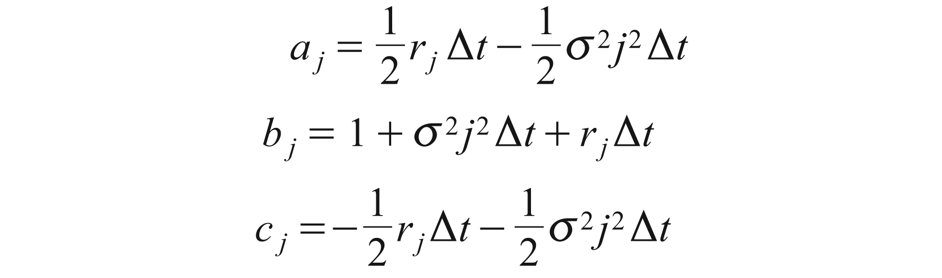
r_j denotes the deterministic probability

σ² denotes the variance of the given sample/sequence

MATLAB codes for the above models have been appended at the end of the study. The simulation results of each of these models with a comparison with the Monte Carlo techniques would be presented in the analysis part.

Monte Carlo Simulation Model

The value of a derivative security in a risk neutral environment is given by the discounted value of its expected terminal date cash flow.

This technique has the following steps involved:

Generate several thousand random price paths for the underlying asset through simulation

Calculating the associated payoff of the option for each price path

Average the payoffs

Discount the payoff to today’s price

The resultant value obtained is the price of the option.

Suppose we want to estimate some ‘θ’ where ‘i’ is given by the following formula as θ = E(g(X)) where g(X) is a function such that E(|g(X)|) < 3 then we can generate n independent random observations with the probability ε (X)

The estimate of i is given by $\overset{}{} \frac{1}{n}_{i 1}^{n} g (X_{i})$ and as n "3 we can say that $\overset{}{}$

To ensure exactness of the sample, we take sample variance into account.

s^{2} \frac{1}{n 1} {_{i 1}^{n} (g (X_{i}) \overset{}{})}^{2}

Quasi-Monte Carlo Simulation Model

The Quasi-Monte Carlo methods converge significantly faster than the Monte Carlo methods. While the Monte Carlo method is sensitive to the initial seed, Quasi-Monte Carlo method uses low discrepancy series which show relatively low dependency on the initial seed. The convergence of Quasi-Monte Carlo is smoother than the convergence of Monte Carlo. This makes automatic termination easier for Quasi-Monte Carlo simulation.

The Quasi-Monte Carlo approach is very similar to the Monte Carlo approach, but it has several advantages over the plain Monte Carlo approach. Quasi-Monte Carlo method is used for low discrepancy sequences. For low discrepancy patterns, the study uses standard normal uniform distribution to ensure that the deviation from mean would be small in magnitude.

Monte Carlo is a randomised method while Quasi-Monte Carlo is purely deterministic, which do not even attempt to follow the behaviour of the independent uniform random variables. We compute the integral over the continuous interval in the Quasi-Monte Carlo approach unlike discrete points in the Monte Carlo approach. The error is minimised because every path is a low discrepancy series of points whose values are obtained using uniform normal distribution.

The generalised equation of a Quasi-Monte Carlo simulation is given by $^{OMC} (f) \frac{1}{n}_{i 1}^{n} f (x_{i})$ which is very similar to the Monte Carlo simulation. Each point in the Quasi-Monte Carlo simulation belongs to a low discrepancy series of numbers. The error in the worst case of the simulation is given by $(\frac{(\log n)^{d}}{n})$ where n is the number of sample points.

The convergence of the simulation is dependent on ‘d’. Large values of ‘n’ make log n devastatingly high, but this value is smaller while compared to the plain Monte Carlo method. For log n as 2 suppose, when ‘d’ is large say 360 the value of (log n)^d becomes extremely high, that is, 2³⁶⁰ and this would make the error very large. Thus we can conclude that the integral in the Quasi-Monte Carlo simulation can be used only for small values of ‘d’. In general, whenever d is less than 10 (d < 10) Quasi-Monte Carlo method converges more accurately and quickly than the Monte Carlo method.

The study also uses the d-dimensional Halton low discrepancy series and d for this case is less than 10. The one-dimensional Halton sequence is constructed within the interval [0,1].

∞

An element of this sequence is calculated by using the following equation: x_i = ± Σn_k–ip^–k–1

k = 0

∞

Where i > 0, p = 2 and n_{k, j} determined by the following equation i = ± Σn_{k, i}p^k; 0 ≤ n_{k, i}< p; n_{k, i}∈N. _{k = 0}

The solution of this equation is ‘i’ takes values only in the open interval (0, 1). We illustrate the algorithm by calculating for the first three points.

For, i = 1: n_0,1 = 1, n_k,1 = 0 for every k > 0

For, i = 2: n_1,2 = 1, n_k,2 = 0 for every k ≠ 0

For, i = 3: n_0,3 = n_1,3 = 1, n_k,3 = 0 for every k > 0

Therefore we get the sequence $\frac{1}{2}, \frac{1}{4}, \frac{3}{4}, \frac{1}{8}, \frac{5}{8},$ ..... This scheme can be extended to higher dimensions as follows. For every dimension j = 1,2,3...d we define x^j by $x_{i}^{j}_{k 0}^{} n_{k, j} (j) p_{j}^{k 1}$ with p_j as the j^th smallest prime number and with n_{k, i} (j) is calculated as follows.

i_{k 0}^{} n_{k, i} (j) p_{j}^{k}

Analysis and Observations

The present study seeks to analyse Asian options pricing through Quasi-Monte Carlo approach and compare the results obtained with that of the binomial tree method, finite-differences method and Monte Carlo method.

The MATLAB codes of the each models has been appended in the appendix. Please refer to Appendix - A for the codes.

First stage of the present study is to start with simulation by generating pseudo random variables in case of Monte Carlo and quasi pseudo random variables in case of Quasi-Monte Carlo.

After generating random variables, the study concentrates the next stage of analysis by pricing Asian options using Monte Carlo method. For an Asian call option, the study generates 10,000 simulated paths to price the option. The algorithm is the following:

Set sum = 0

For i = 1 to n

Generate S (T/m), S (2T/m)... S(T)

Set sum = sum + max (0, $\frac{_{i 0}^{m} S (\frac{iT}{m})}{m 1} K$ )

End

Set C^{k, a} = exp (-rT) sum/n

The above algorithm is given for an arithmetic call Asian option, for a put option the equation of sum changes to sum = sum + max (0, $K \frac{_{i 0}^{m} S (i \frac{iT}{m})}{m 1}$ )

For a geometric average Asian option, the study didn’t use the sum directly, but the algorithm is modified by using variance as the geometric mean is considered. The study uses a control variate given by V = e^{–rT
${(e^{\frac{1}{m 1}_{i 0}^{m} S (\frac{iT}{m})} K)}^{}$}. The equation is valid only for a call option, for a put the equation is modified as V = e^{-rT
${(K e^{\frac{1}{m 1}_{i 0}^{m} S (\frac{iT}{m})})}^{}$}

Table 1.

Asian Call Option with Geometric Payoff Using Monte Carlo Method

k	m	Geometric Asian Call	Option Value	Standard Error
80	10	12.253	12.612	0.1293
	50	12.302	12.656	0.1288
	100	12.368	12.669	0.1243
	500	12.382	12.701	0.1258
100	10	5.327	5.483	0.0562
	50	5.349	5.503	0.0560
	100	5.377	5.508	0.0541
	500	5.393	5.522	0.0547
120	10	1.522	1.567	0.0361
	50	1.528	1.572	0.0360
	100	1.536	1.574	0.0354
	500	1.538	1.578	0.0356

Source: Computed.

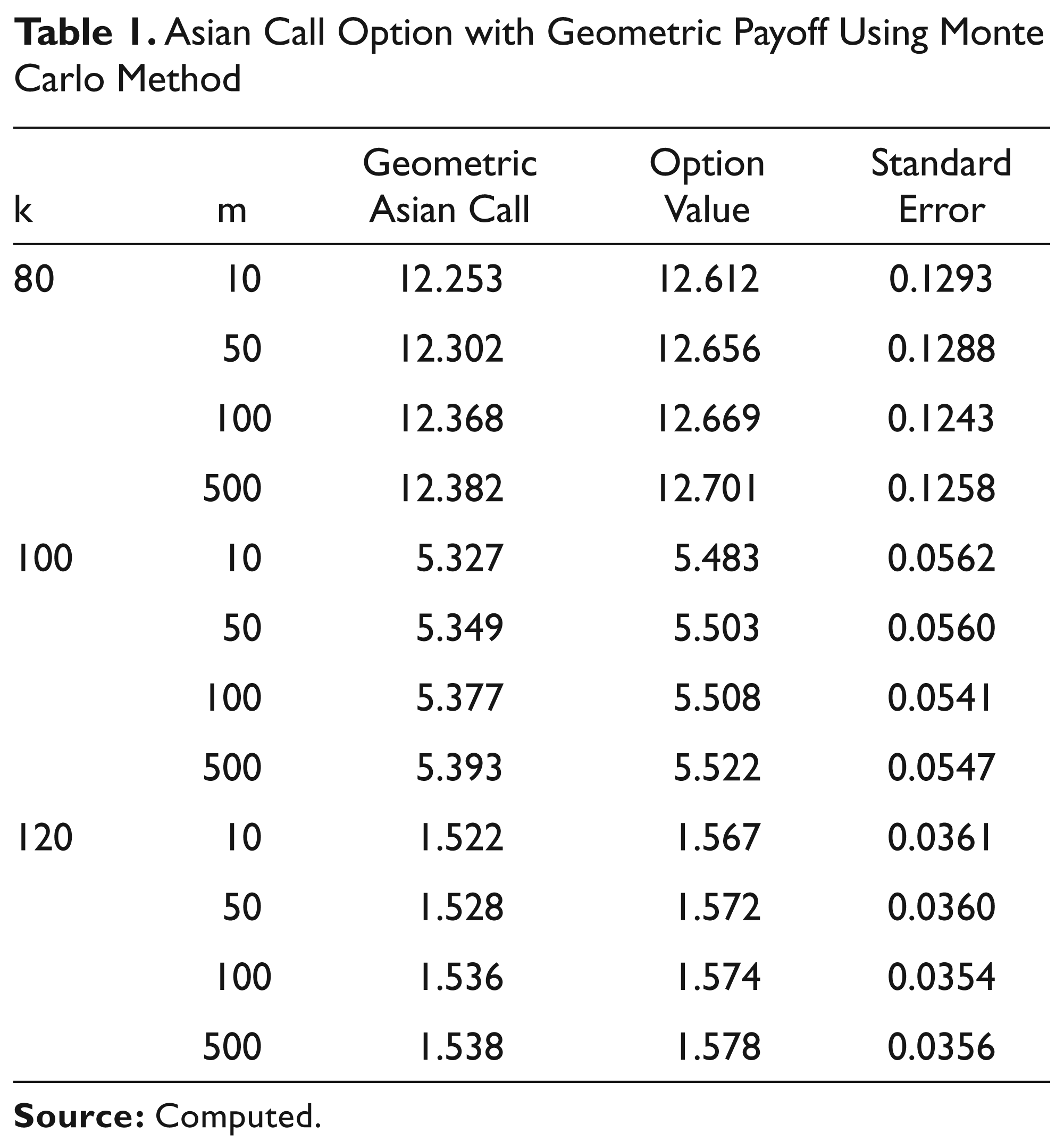
From Table 1, the study finds that the value of the strike price increases, the option price decreases and standard error observed is also decreases with an increase in the strike price.

Using Quasi-Monte Carlo approach, the study generates the quasi pseudo random numbers using ‘Haltonset’ and ‘qrandset’ function in MATLAB. It uses the Halton series (explained in Quasi Monte Carlo Simulation Model section) to generate quasi pseudo random sequences. Once the sequences are generated, the study needs to determine the associated payoff for each path and then to find the arithmetic average of the payoff. Finally, discount it to present value to price the option. The algorithm is similar to that of the Monte Carlo except for the input variables which are the quasi pseudo random sequences.

The MATLAB code for the Quasi-Monte option pricing method is attached in the Appendix.

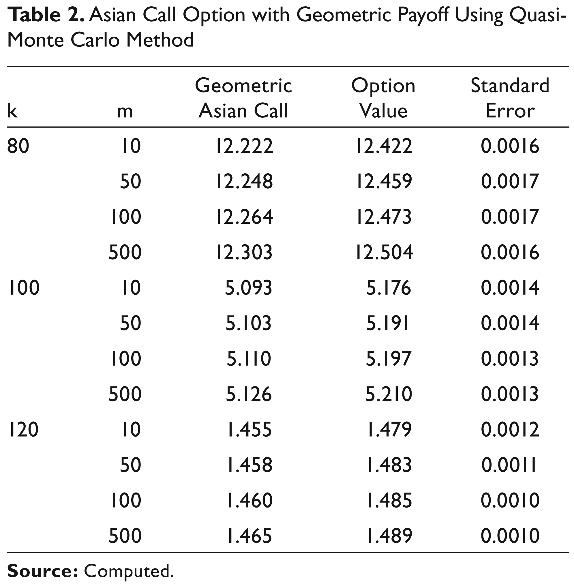
From Table 2, the study finds that the option prices are similar to that of the Monte Carlo method, but the standard error is less. This means that the results are more accurate. Also the study finds that the ‘m’ number of paths increases which led to decrease in the standard error. This shows that the convergence is high for this approach. The standard error of the Quasi-Monte Carlo approach is much lesser than that of the Monte Carlo approach.

Table 2.

Asian Call Option with Geometric Payoff Using Quasi-Monte Carlo Method

k	m	Geometric Asian Call	Option Value	Standard Error
80	10	12.222	12.422	0.0016
	50	12.248	12.459	0.0017
	100	12.264	12.473	0.0017
	500	12.303	12.504	0.0016
100	10	5.093	5.176	0.0014
	50	5.103	5.191	0.0014
	100	5.110	5.197	0.0013
	500	5.126	5.210	0.0013
120	10	1.455	1.479	0.0012
	50	1.458	1.483	0.0011
	100	1.460	1.485	0.0010
	500	1.465	1.489	0.0010

Source: Computed.

Table 3.

Asian Call Option Pricing Using Binomial Tree Model

K	Option Value	Standard Error
80	13.156	0.1245
100	6.432	0.1209
120	1.983	0.1168

Source: Computed.

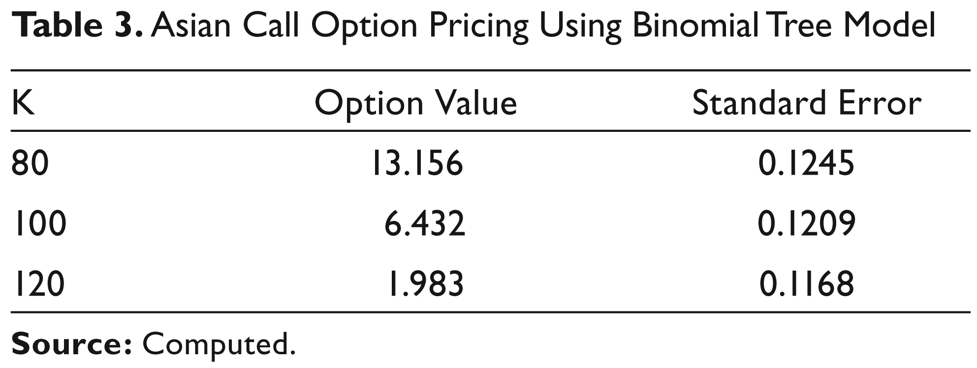
For binomial model, the study needs to generate the tree. The study has used the special that the study generates Asian options using ‘crrbytree’ function.

For the binomial tree model, the study calculated options price at each knot and finds that the final price is greater than the price obtained in the Monte Carlo models. Also the error being higher, so using binomial tree model for pricing Asian options is insignificant (Refer the Appendix for MATLAB code).

For finite-differences method, the study uses equations developed in section 5.4 to generate the option prices at the end of the maturity period. Calculating the values of each of the constants, the study prices the options by substituting the initial conditions back in the generated equation. For a geometric call Asian option, the study uses the Crank-Nicolson finite-difference method because it consists of both implicit as well as explicit variables and it needs to be accounted for.

From Table 4, the study finds low standard error, so finite-difference model can be used to price Asian options, for an average geometric payoff.

Table 4.

Asian Call Option Pricing Using Finite-difference Model

K	Option Value	Standard Error
80	12.745	0.022
100	5.594	0.019
120	1.576	0.014

Source: Computed.

Comparing the Results of the Different Models

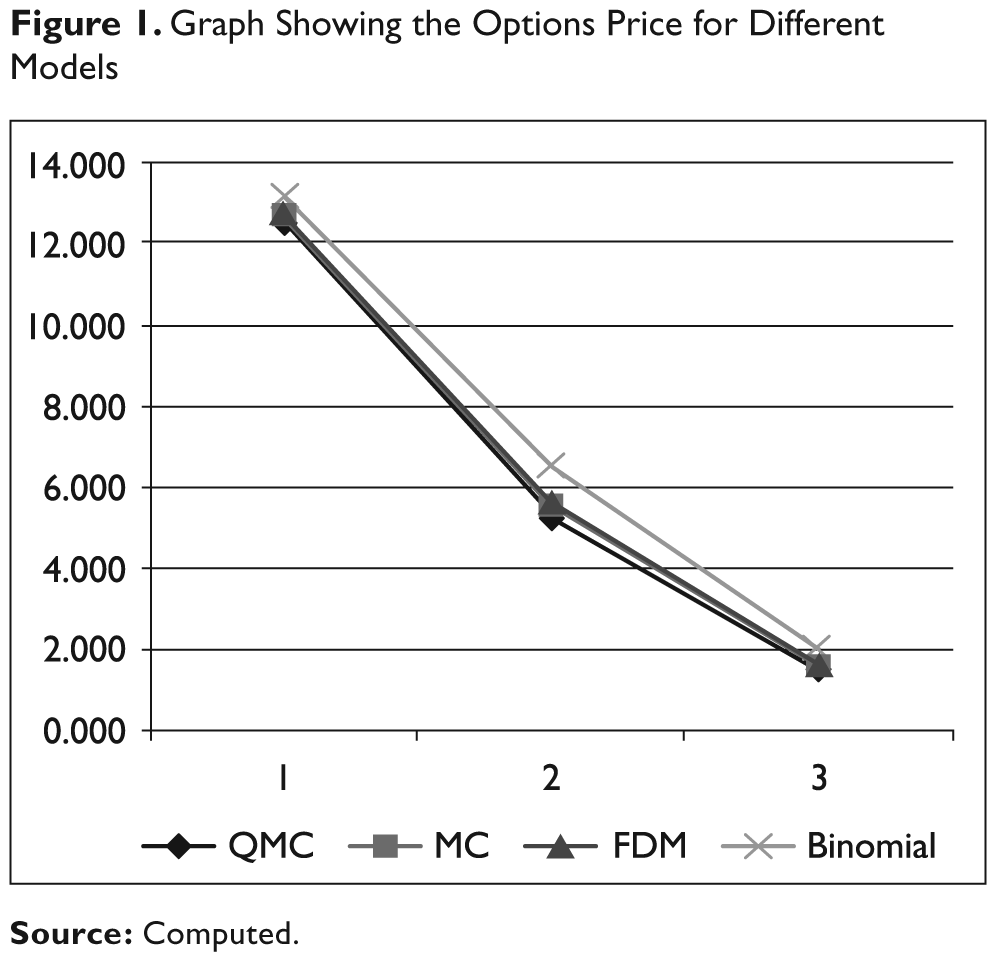
Now, the study needs to compare the results from the convergence pattern of the different sets of values obtained from various models for the purpose of identifying the best model for pricing the options.

Figure 1 also clearly indicates that the options price estimated from the binomial model is higher than that of the other models. While the remaining three models show almost similar values but Quasi-Monte Carlo method gives the best approximation to the options price which can be obtained from Figure 1.

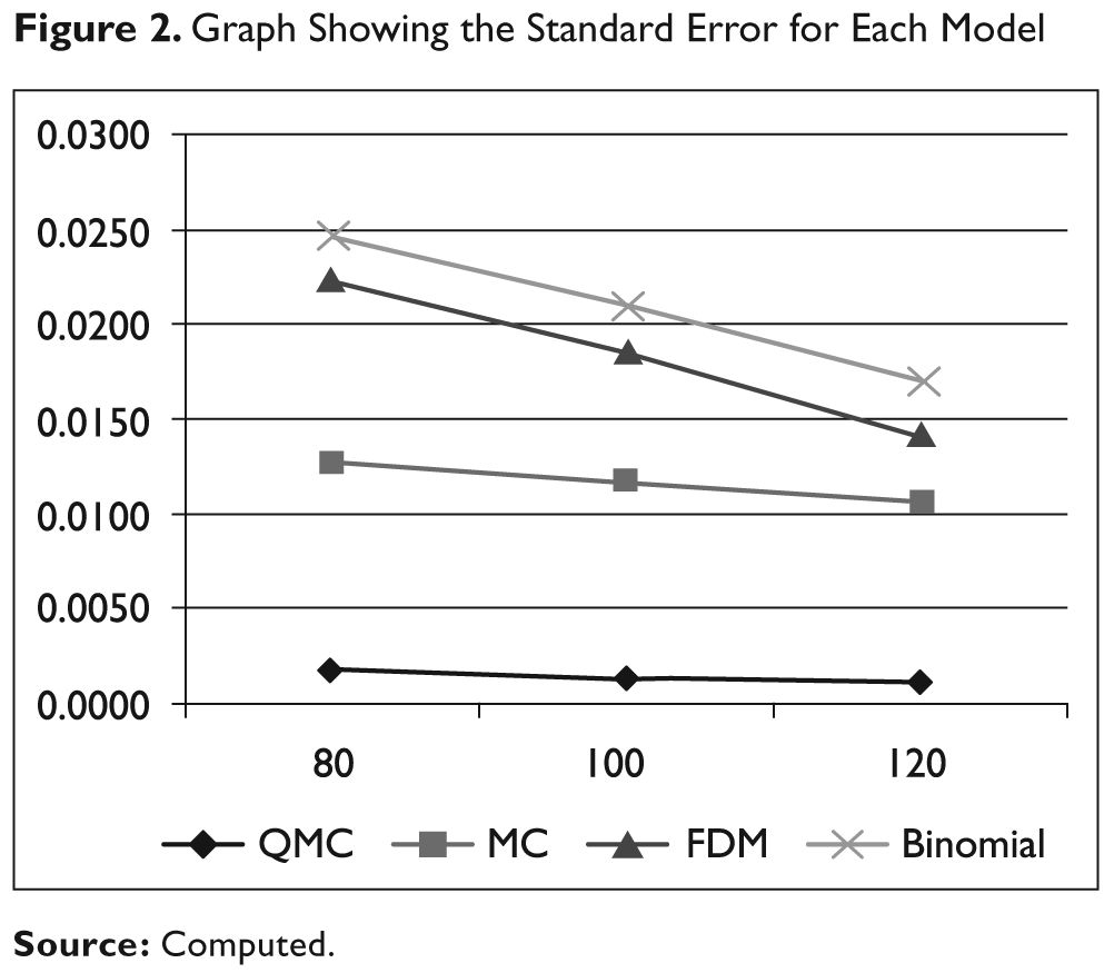
It is very obvious from Figure 2 that the standard error in the Monte Carlo methods is lower than the other models. Comparing the Monte Carlo, finite-difference and binomial models, the study finds that the minimum standard deviation is found when the Monte Carlo model is used, while the maximum error is observed in case of binomial model. This implies that the convergence to the accurate value is observed more in case of Monte Carlo model but Quasi-Monte Carlo model gives us results with high precision.

Figure 1.

Source: Computed.

Figure 2.

Source: Computed.

Summary and Conclusions

This article aimed at pricing options using Quasi-Monte Carlo methods and compares the results with other models to identify the exact model for options pricing. According to the hypothesis, as large numbers of paths are required for high precision and convergence, the study finds that the obtained results are in accordance with our hypothesis. With less number of sampling paths, the convergence to the accurate value was less relative to that of more number of paths. Precise results were obtained when the study used path independent log normally distributed quasi random sequences. The results also show that the Quasi-Monte Carlo approach is superior over the other models for options pricing. Asian options involve a complexity of averaging payoff over time, which create discrepancies when pricing with binomial trees causing large errors. Finite-difference method is a close substitute of the Monte Carlo method and gives very similar results.

Simulations direct us towards a new path of innovation and experimentation. Different exotic options can be easily priced using simulations. In the modern era of high technological growth, an approach towards derivatives through simulations would build a brighter path for the advancement in the area of derivatives.

Asian options are just a single set of exotic options; there is a tremendous amount of future scope in this field with different kinds of other options which include the Bermudian options, vanilla options, barrier options, look-back options, volatility options and Parisian options.

Footnotes

Appendix

MATLAB Code of Binomial Model for Asian Options Pricing for Call Option

MATLAB Code of Finite-difference Model for Asian Options Pricing for Call Option

MATLAB Code of Monte Carlo for Asian Options Pricing for Call Option

MATLAB Code of Quasi-Monte Carlo for Asian Options Pricing for Call Option

References

Addae

(2006). The pricing of Asian options. Unpublished Honours thesis, University of Cape town, South Africa.

Avramidis

Athanassios N.

L’Ecuyer

Pierre

. (2006). Efficient Monte Carlo and Quasi-Monte Carlo option pricing under the variance-gamma model. Management Science, 52(12), 1930–1994.

Dion

L’Ecuyer

(2010). American option pricing with randomized quasi-Monte Carlo simulations. Proceedings of Winter Simulation Conference, 2705–2720.

Michael C.

Madan

Dilip B.

Wang

Tong

(1997). Pricing Asian options: A comparison of analytical and Monte Carlo methods. The Journal of Computational Finance, 32(4), 1–28.

Fusai

(2004). Pricing Asian options via Fourier and Laplace transform. Journal of computational finance, 7(3), 87–106.

Jasra

Ajay

Moral

Pierre Del

(2011). Sequential Monte Carlo methods for options pricing. Stochastic Analysis and Applications, 29(2), 292–316.

Jia

Quiji

(2009). Pricing American options using Monte Carlo methods. Sweden: Department of Mathematics, Uppsala University.

Lai

Spanier

(1998). Applications for Monte Carlo & Quasi-Monte Carlo methods in finance: Option pricing. In Niederreiter

Spanier

(Eds), Monte Carlo and Quasi Monte Carlo methods (pp. 284-295). Springer-Verlag.

Nielsen

J. A.

Sandmann

Klaus

. (2003). Pricing bounds on Asian options. Journal of Financial and Quantitative Analysis (JFQA), 38(2), 449–473.

10.

Petroni

Nicola Cufaro

Piergiacomo

Sabino

(2013). Pricing and hedging Asian basket options with Quasi Monte Carlo. Methodology and Computing in Applied Probability, 15(1), 147–163.

11.

Ribeiro

Webber

(2002). A Monte Carlo method for the normal inverse gaussian option valuation model using an inverse gaussian bridge. Computing in Economics and Finance, 5(1), 1–15.

12.

Vazquez-Abad

F. J.

Dufresne

(1998). Accelerated simulation for pricing Asian options. Proceedings of the 30th conference on winter simulation, IEEE computer society press, pp. 1493–1500.

13.

Vecer

(2000). Unified pricing of Asian options. New York: Department of Statistics, Columbia University. Retrieved from http://www.stat.columbia.edu/~vecer/asian-vecer.pdf

14.

Vecer

(2001). Pricing Asian options in a semimar Tingale model. Preprint.

15.

Vorst

A. C. F.

(1996). Averaging options. In Nelken (Ed.), Handbook of exotic options (pp. 362–374), I. Irwin, Chicago.