Linking Attentional Modulation to Auditory Attention Decoding: Using Colocated Stimuli With a Fixed Temporal Structure

Introduction

Selective attention plays a role in tracking auditory objects (e.g., target speech) while filtering out distracting sounds. Top-down attention is important for maintaining continuous tracking of the speech stream, whereas bottom-up attention is important for detecting salient events (Huang & Elhilali, 2020). In a cocktail party situation (Cherry, 1953) with multiple talkers, top-down attention is especially critical, given that the saliency of the target and distractor (e.g., loudness, pitch, or location) can be very similar. Indeed, top-down selective attention performance was found to be correlated with speech perception in the presence of competing talkers (Oberfeld & Klöckner-Nowotny, 2016; Tierney et al., 2020).

Accordingly, an important step toward characterizing auditory attention is to measure the magnitude of top-down attentional modulation in neural responses, thereby providing a foundation for subsequent approaches that aim to decode or model attention directly from brain activity.

Evidence for this attentional modulation is found in several neural correlates of selective attention. Classical event-related potential (ERP) studies have shown that the cortical neural responses are modulated by top-down attention. For example, N1 peaks, negative peaks around 100 ms after the sound onset, and P2 peaks, positive peaks following the N1 peak, are increased when the stream is attended compared to when it is ignored (Choi et al., 2013; Hillyard et al., 1973; Woldorff & Hillyard, 1991). Neural entrainment to target speech is also modulated by top-down attention (Ding & Simon, 2012; Fiedler et al., 2019; Golumbic et al., 2013; Mesgarani & Chang, 2012; Power et al., 2012). Slow neural oscillations like delta (1–4 Hz) and theta (4–8 Hz) frequency bands from the auditory cortex, for example, are entrained to the attended speech stream (Etard & Reichenbach, 2019; Kerlin et al., 2010; Viswanathan et al., 2019).

The attentional modulation index (AMI) is a measure developed to quantify the degree of attentional modulation of neural responses and has been computed in several ways. For ERP studies, AMI was calculated as the ratio of ERP component amplitudes between attended and ignored conditions, averaged across all target onsets (Dai & Shinn-Cunningham, 2016; Lee et al., 2022). This quantifies the amplitude change when the target sound is attended relative to when it is ignored, as defined by the formula: a t t e n d e d − i g n o r e d a t t e n d e d + i g n o r e d (Lee et al., 2022; Tune et al., 2021). For neural entrainment studies, AMI was calculated by subtracting the correlation of the neural response to the distractor speech from the correlation to the target speech (Mesgarani & Chang, 2012; O'Sullivan et al., 2019), as shown in the formula: c o r r ( S p k 1 a t t e n d , S p k 1 a l o n e ) − c o r r ( S p k 1 a t t e n d , S p k 2 a l o n e ) +

c o r r ( S p k 2 a t t e n d , S p k 2 a l o n e ) − c o r r ( S p k 2 a t t e n d , S p k 1 a l o n e ) (O'Sullivan et al., 2019).

Importantly, AMI is associated with the behavioral performance of selective attention (Choi et al., 2014; Dai & Shinn-Cunningham, 2016) and also speech-in-noise perception (Choi et al., 2014; Kim et al., 2021; Kurthen et al., 2021; Schmitt et al., 2022; Tune et al., 2021). For instance, word-in-noise performance was correlated with AMI in young adults with normal hearing (Kim et al., 2021) and in cochlear implant users (Berger et al., 2023; Lee et al., 2022). From 151 age-typical hearing participants, Tune et al. (2021) found that higher AMI is correlated with accuracy and speed of speech perception. Speech comprehension was positively correlated with the amplitude of the late peak of the temporal response function (TRF; Kurthen et al., 2021). The degree of cortical neural tracking was correlated with speech comprehension in older adults (Decruy et al., 2019) and in older adults with hearing loss (Decruy et al., 2020; Schmitt et al., 2022).

Based on attentional modulation, researchers developed an algorithm that can identify which auditory stream a listener is attending to in a mixture of multiple streams. Such an algorithm is called auditory attention decoding (AAD). Electroencephalography (EEG) has been widely used as a physiological signal for AAD due to its noninvasive and versatile nature. Over the past decade, extensive research has examined methodological frameworks for AAD using EEG (see Belo et al., 2021; Geirnaert et al., 2021; Puffay et al., 2023 for reviews). The frameworks can be categorized into three major classes: ERP-based decoders, linear-model-based decoders, and EEG-feature-based machine-learning decoders.

Early AAD approaches used attentional modulation of ERPs (Choi et al., 2013; Hill & Schölkopf, 2012; Treder et al., 2014), which is well-suited to isolating and characterizing the neural response to time-locked events, such as the onset of a target sound or a distractor. The morphology of ERP components (e.g., P1, N1, P2) can be directly compared across conditions, allowing researchers to pinpoint the timing of processing modulated by attention (Choi et al., 2013). The downside of this temporal precision, stemming from a time-locked design, is that an ERP-based approach cannot incorporate more natural stimuli, such as continuous speech.

Linear model-based decoders utilize the fact that neural representations of the target sound are stronger than those of the distractor sound. Under the assumption that the auditory system is linear and time-invariant, a time-lagged, regularized linear function relating auditory input features (e.g., speech envelope) to the corresponding EEG response can be estimated. A linear model with auditory features as inputs and EEG responses as outputs is called the forward model, encoding model, or TRF. A linear model fitted with EEG responses as input and auditory features as output is called the backward model, decoding model, or stimulus reconstruction model.

To decode attention using the forward model, the attentional modulation is encoded by fitting the model with target speech features and the corresponding attended EEG responses. Attention is then inferred by comparing how closely the actual EEG response resembles the modeled EEG responses predicted from clean speech streams (Wong et al., 2018). Spatial and temporal analyses of the TRF coefficients (or model weights) can be interpreted in terms of neuroscience theories of auditory information processing (Kriegeskorte & Douglas, 2019). The TRF preserves the biophysical plausibility of the system (from sound to brain) and enables direct inspection of model coefficients that resemble auditory evoked responses (Ding & Simon, 2012; Etard & Reichenbach, 2019; Kong et al., 2015; Lalor et al., 2009).

For the backward model, a regularized linear regression is fitted to predict target speech features from the EEG response while a listener attends to the target sound within a mixture. Attention is inferred by comparing whether the correlation of the model-predicted speech features to one speech is higher than the other speech (Mirkovic et al., 2015; O'Sullivan et al., 2015).

A limitation of linear model-based attention decoding is that decoding performance degrades as the analysis window duration decreases, even when the model is trained on the same amount of data (Geirnaert et al., 2021; Wong et al., 2018). Geirnaert et al. (2021) reported that both forward and backward linear models achieve reliable decoding with window lengths of 10–20 s, but performance drops significantly for shorter durations. Another limitation is that the linear modeling approach requires a clean signal of the target sound, which is not always available in a real-world setting.

EEG-feature-based machine learning models, including deep neural networks, have shown promise in this context. Machine learning models can extract nonlinear, high-dimensional features from raw EEG, enabling them to decode attention without a clean audio signal and within a shorter time window (Belo et al., 2021; Geirnaert et al., 2021; Puffay et al., 2023). Various neural network architectures have been implemented for AAD, including: convolutional neural networks (CNNs; Accou et al., 2021; Ciccarelli et al., 2019; Vandecappelle et al., 2021), transformer layers (de Taillez et al., 2020; Li et al., 2022; Su et al., 2022; Xu et al., 2022), and graph-convolution layers (Cai, Zhang, & Li, 2024), and the combination of multiple architectures (Wang et al., 2023). Several studies have reported strong decoding performance with windows as short as 1 s and, in some cases, as brief as ∼200 ms (Su et al., 2022; Wang et al., 2023; Xu et al., 2022).

The inherent challenge of the EEG-feature-based machine learning approach is explainability. They do not rely on assumptions of attentional modulation and may learn spurious correlations unrelated to underlying cognitive processes. For example, Rotaru et al. (2024) demonstrated that machine learning models trained on EEG data from spatial selective attention tasks can overfit to nonneural artifacts, such as eye-gaze or other confounds, that are associated with trial order. This is problematic, given that the vast majority of deep learning-based decoders have been trained on public datasets that lack carefully controlled eye-gaze or trial-order conditions, indicating that reported within-subject performance levels may be inflated and that decoding results would not generalize to new EEG data.

In this regard, it is important to inspect which EEG features AAD algorithms rely on. If we cannot verify that the AAD is based on neural markers of attentional modulation, its generalizability across populations may be limited. Interpretability is also crucial when employing such decoding schemes for neuroscientific interpretation or explanation. As noted earlier, attentional modulation of neural responses is a well-established observation associated with top-down attentional control of sensory processing. Linear model-based decoders inherently capture this attentional modulation by design, whereas machine learning models are not constrained by such assumptions. Therefore, investigating whether EEG-feature-based machine learning models primarily rely on attention-modulation features in a well-controlled experimental design would provide insight into developing AAD algorithms with improved generalizability and explainability.

Therefore, we aimed to investigate how ERPs and AMI relate to (and can help interpret) attention decoding performance across linear model-based pipelines and a CNN. For this purpose, we fit AAD models to EEG data from an auditory selective-attention experiment using a colocated two-stream paradigm with a fixed temporal structure. Simple, repetitive stimuli enable clear ERP isolation and AMI computation, which serve as ground-truth features that we want our AAD model to learn. The colocation of two audio streams minimizes confounding variables such as eye-gaze biases. A short 4-s time window enables us to compare the performance of linear model-based decoders and a CNN decoder; both algorithms still perform above chance, but with distinct differences. It also enables us to explore near-real-time applications. We investigated the extent to which the AAD algorithm relies on attentional modulation features by comparing its output with established attentional modulation markers of the N1-P2 peaks and AMI. We assumed that if the classifier learned to differentiate the single-trial EEGs based on this feature, the averaged neural response from correctly classified trials would display more prominent attentional modulation than the averaged response from incorrectly classified trials. Additionally, if successful decoding is associated with an individual's strength of attentional modulation, a significant correlation between AMI and the attention decoding performance will be observed in each participant's EEG data.

We hypothesized that, consistent with previous findings (e.g., Puffay et al., 2023), the CNN decoder would outperform linear-model-based decoders in attention decoding accuracy, particularly for short time windows. We also expected the linear model-based decoders would provide a clearer association to known auditory evoked response components and AMI.

Method

Data Collection

Participants

We recruited 28 participants (five males, 23 females) aged 20–44 years (mean = 23.86, standard deviation [SD] = 5.81) from the student population at the University of Iowa. Nineteen were right-handed, six were left-handed, and three had unknown handedness. All had normal hearing thresholds (below 20 dB HL) at the octave frequencies from 250 to 8000 Hz. The University of Iowa Institutional Review Board reviewed and approved the experimental procedures.

Task Design

During the experiment, participants listened to two simultaneous four-second speech streams: a female voice repeating “Up” every 0.8 s for five repetitions, and a male voice repeating “Down” every second for four repetitions (Figure 1). Their task was to focus on a designated target speech stream and ignore the other stream. Within each “Up” and “Down” stream, one utterance had a 26% (four semitone) higher pitch, occurring at either the third, fourth, or fifth position. Participants identified the position of this high-pitched utterance in the target stream by pressing the corresponding number on a keypad at the end of the trial. For example, if the third “Up” and the fourth “Down” had a higher pitch, and the target was “Down,” the participant would have to press “4” to be correct. Sound was presented via a loudspeaker at 70 dB SPL.

OPEN IN VIEWER

Figure 1.

Trial structure of the task. The participants were instructed which speech stream was the target (e.g., “Down”). White noise was presented first, and after 0.5 s, both “Up” and “Down” sounds were played from the same location, using different voices. One of each “Up” and “Down” was high-pitched (e.g., fourth “Up” and second “Down”). At the end of the trial, participants had to press number keys to answer which word was “odd” in the target speech stream (e.g., 2).

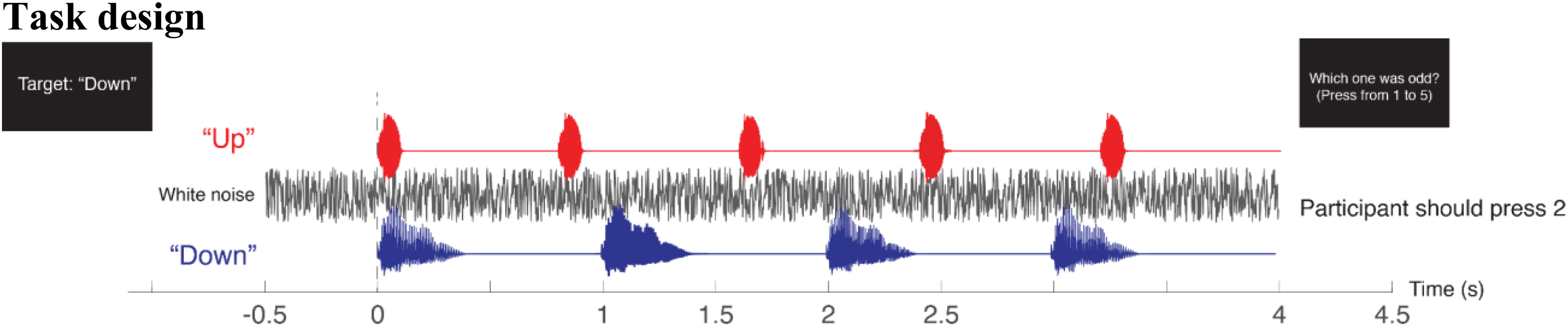
The experiment consisted of 120 trials, with 60 trials each for the “Up” and “Down” targets. Each trial began with a 0.5-s display showing the current trial number out of the total (e.g., Trial 3/120). Subsequently, a visual cue was presented for 1.5 s, indicating the target speech stream (e.g., “Target: Down”). The target order was randomized across trials. Following this, a fixation cross (“+”) was presented on the screen; participants were instructed to maintain focus on the fixation cross throughout each trial to minimize eye movements. Two speech streams were presented 2 s after the white cross appeared. To reduce auditory onset responses, white noise (bandwidth of 0–22050 Hz) at 17 dB SNR was played preceding the speech onset by 0.5 s and accompanied until the end of speech stream. After each trial, participants received visual feedback (“Correct” or “Incorrect”) indicating the correctness of their response. The subsequent trial began after a 0.6 s pause.

We ran the task using the Psychtoolbox 3 package (Brainard, 1997; Pelli, 1997) from MATLAB (R2020b, The MathWorks). All tasks were conducted in a sound-treated, electrically shielded booth. A computer display located 0.5 m in front of the participant at eye level provided all visual cues.

EEG Acquisition and Preprocessing

Electrical brain activity was recorded using a BioSemi ActiveTwo system at a 2048 Hz sampling rate. Sixty-four active electrode channels were placed on the scalp using an elastic cap following an international 10–20 configuration. Time-locked triggers were sent via MATLAB to the “BioSemi ActiView” acquisition software.

Epochs were extracted from −1.5 to 5 s relative to the onset of the speech stimulus. The signal was baseline-corrected using the average voltage from −0.7 s to −0.5 s. Then, the epochs were downsampled to 256 Hz. Noisy trials and channels were removed from the data based on the histogram of maximum voltage across all trials and channels. For each subject, the rejection threshold was determined by examining the distribution of the maximum voltage across trials (Luck, 2014), based on a bimodal Gaussian-mixture fit to the histogram. The mean number of rejected trials was 4.82 (SD = 7.59). The same procedure was applied to the channel-wise maximum value, yielding a mean of 1.11 rejected channels per participant (SD = 0.73).

Artifacts related to eye movements were identified using infomax independent component analysis (ICA) in the EEGLAB toolbox (v2022.1; Delorme & Makeig, 2004) and removed by human inspection. On average, two ICA components have been removed per subject (mean = 1.82, SD = 0.39). The referencing scheme prior to artifact removal was connected mastoid referencing. After artifact removal, EEG signals from the removed channels were interpolated using the spherical spline method (Perrin et al., 1989) in MNE-Python (v1.4; Gramfort et al., 2014). Then, each epoch was re-referenced to the average across all channels. An FIR bandpass filter (1–15 Hz) was applied to isolate the envelope-following response of the EEG. Epochs between 0.5 and 4 s were used for further analysis. This was to exclude periods during which neural responses were unrelated to speech, reduce edge effects from filtering, and mitigate the model's overfitting to the strong onset response. Finally, the EEG was downsampled to 64 Hz to reduce computational costs.

Decoding of Selective Attention

Linear Modeling

Neural tracking of speech was characterized by estimating linear mappings between the auditory stimulus and neural responses (Bialek et al., 1991; Lalor et al., 2009). This study employed both forward (encoding) models to reconstruct EEG signals from the speech envelope and backward (decoding) models to reconstruct the envelope from multi-channel EEG activity. The analytic envelope of the speech signal was calculated via Hilbert transform and downsampled to 64 Hz. All linear modeling was implemented using the “mne.decoding.ReceptiveField” function in MNE-Python (v1.4; Gramfort et al., 2014), with integration time lags set to 0.0–0.4 s for the forward models and −0.4–0.0 s for the backward models.

Model weights were estimated using ridge regression. Specifically, the solution was defined as W = ( X T X + λ I ) − 1 X T Y , where X and Y represent the input and output signals of reconstruction, respectively. A nested cross-validation scheme was implemented to optimize the regularization parameter λ and minimize overfitting. In the outer loop, a leave-one-subject-out procedure was used to isolate a test set. In the inner loop, the remaining data were randomly split into ten subsets; one subset served as a validation set to evaluate λ across a search range of 10 − 2 to 10 9 . The optimal λ values from these ten folds were averaged and applied to the final linear model estimation used for the attention decoding.

The reconstruction performance of each model was quantified using the Pearson correlation coefficient (r) between the reconstructed and actual signals. For the forward model, correlation coefficients were calculated for each of the 64 EEG channels and then averaged to provide a single global measure of model fit. For the backward model, performance was assessed by correlating the reconstructed envelope with the original speech envelope for both attended and ignored conditions. Statistical differences in tracking performance between conditions were evaluated using paired t-tests.

To assess the attentional modulation of neural tracking, we fitted the linear model using either “attended” or “ignored” speech envelopes and compared their model fit. For each trial, an attended model was estimated by mapping the EEG signals to the envelope of the target speaker (e.g., the “Up” envelope when the participant was instructed to attend to the “Up” speaker). Conversely, an ignored model was estimated using the same EEG data but mapped to the envelope of the distractor speaker (e.g., the “Up” envelope when the participant was attending to the “Down” speaker). To ensure comparability of the model fits across conditions and participants, a fixed regularization parameter of 10 4 was used, which was the λ value that showed the maximum model fit between the range of 10 − 2 to 10 9 . For forward TRF we examined the reconstruction performance and the absolute amplitudes of weights at latency peaks between 50 ms and 200 ms, which are approximations of auditory N1 and P2 responses.

Forward Linear Model With a Machine Classifier

After estimating the TRF, we convolved it with each speech envelope to predict the EEG signals. The correlation coefficients ( r score) between actual and predicted single-trial EEG signals of all 64 channels were used as input features for attention decoding (Wong et al., 2018). The r scores were computed from one actual EEG and two predicted EEGs, one derived from each competing speech envelope for the “Up” and “Down” streams. Therefore, the total number of input features was 128—64 Channels × 2 Speech Streams. Based on these features, the classifier had to predict whether the target speech of the trial was “Up” or “Down.” The classifier was trained using a leave-one-subject-out approach. We used two binary classifiers: logistic regression and a support vector machine classifier (SVC) with a radial basis function kernel, implemented with the “scikit-learn” package (v.1.3.1; Pedregosa et al., 2011). Figure 2 is a diagram depicting this process.

OPEN IN VIEWER

Figure 2.

Attention decoding process with the forward model (TRF) and machine classifier. Two speech envelopes from “Up” stream and “Down” stream were convolved separately with the pretrained forward TRF coefficients, resulting in two reconstructed EEG signals. The correlation coefficients between the two reconstructed EEG signals and the actual single-trial EEG signal were computed for each EEG channel. The resulting correlation coefficient matrix was then used as input to the machine-learning classifier, either logistic regression or SVM. The classifier determined whether the corresponding correlation pattern more closely matched attending “Up” or “Down.”

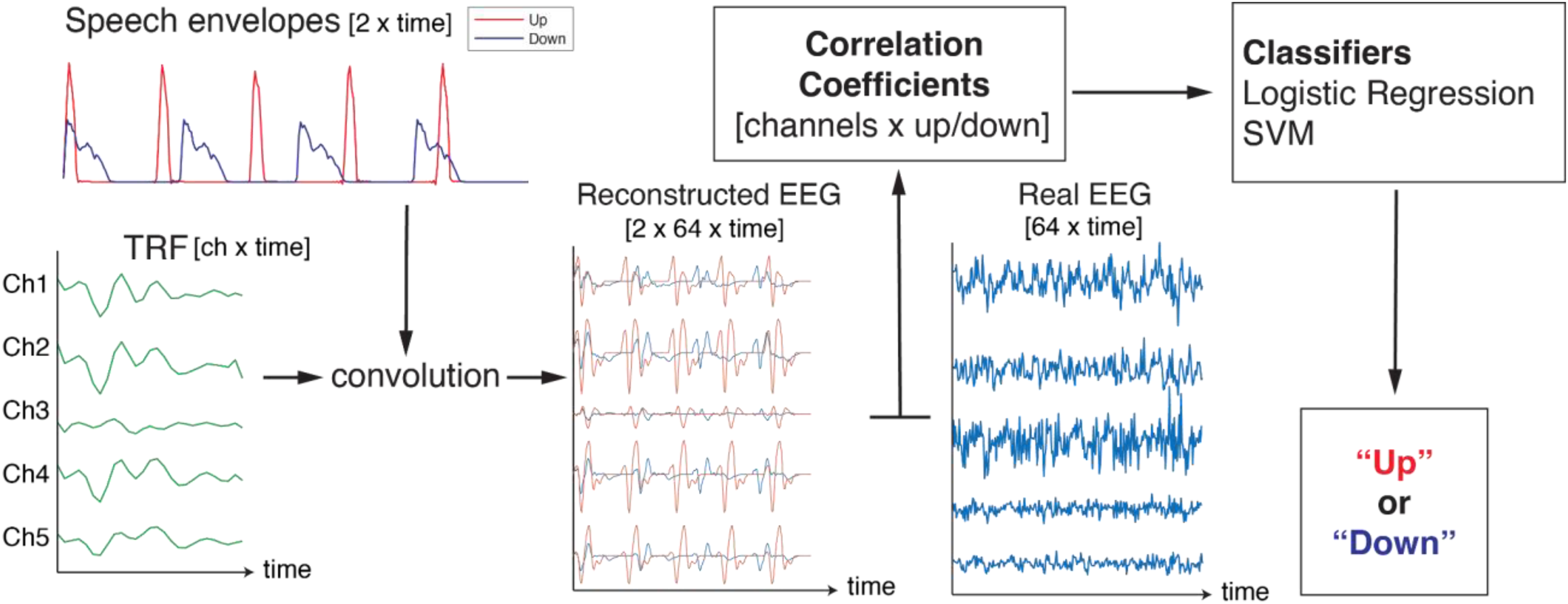
The hyperparameters of logistic regression and SVC were optimized via grid search using 10-fold cross-validation on the training set. For logistic regression, the C value, which controls the strength of regularization, was searched across a range of 10 − 5 − 10 3 . The regularization method was selected between l 1 and l 2 . For SVC, the C value was searched between 10 − 4 and 10 6 . The gamma value, which decides the complexity of the decision boundary, was selected between 1 / N f e a t u r e s and 1 / ( N f e a t u r e s V a r ( X ) ) , where N f e a t u r e s denotes the number of features (which is 64 Channels × 2 Speech = 128 here), and V a r ( X ) is the variance of the input data.

Backward Linear Model

To determine the attended speech stream, we calculated the correlation coefficient ( r score) between the reconstructed attended speech envelope and both the target and distractor speech envelopes. Each trial was then classified based on the higher r score. For instance, if the correlation between the reconstructed envelope and the “Up” stream was stronger than that with the “Down” stream, the trial was classified as attention to “Up.” This backward modeling approach follows the method introduced by O'Sullivan et al. (2015).

Convolutional Neural Network

Our CNN model (Figure 3) used a simple two-layer structure, implemented in PyTorch. The main operation of each layer consisted of one-dimensional convolution for feature extraction, activation function (ReLU) for introducing nonlinearity, dropout for regularization, and batch normalization for training stability. The first layer reduced the 64-channel EEG waveform into eight channels, with a convolution kernel size of 2, a stride of 2, and a dropout rate of 39.4%. The second layer reduced the number of channels from 8 to 3, with a kernel size of 1, a stride of 1, and a dropout rate of 45%. After two convolutional layers, the model flattened the input into a one-dimensional matrix by stacking the rows. This allowed the data to be passed through a linear matrix multiplication layer, which maps the input to only two values, corresponding to the model's confidence that the attended stream was “Up” or “Down.” These values were then passed through a softmax layer to produce two logits, each ranging from 0 to 1 and summing to 1. The final prediction was made based on whichever logit is higher. The hyperparameters of the model (the number of layers (blocks), kernel sizes of the convolution layers, number of channels at each layer, dropout rates, learning rates, and weight decay values for the training process) were optimized using the Optuna package (Akiba et al., 2019). We conducted a grid search using this package, which iterates over random hyperparameter settings, evaluates the resulting accuracy, and then adjusts the hyperparameters for subsequent iterations.

OPEN IN VIEWER

Figure 3.

Block diagram of convolutional neural network architecture. The time-by-channel EEG waveforms were the input to the CNN decoder. The EEG waveforms were passed through two layers of one-dimensional convolutional blocks. Each convolutional block was followed by a ReLU activation, Dropout, and Batch Normalization. The output of the second layer was flattened and mapped to the two output labels (“Up” or “Down”) using a Softmax function.

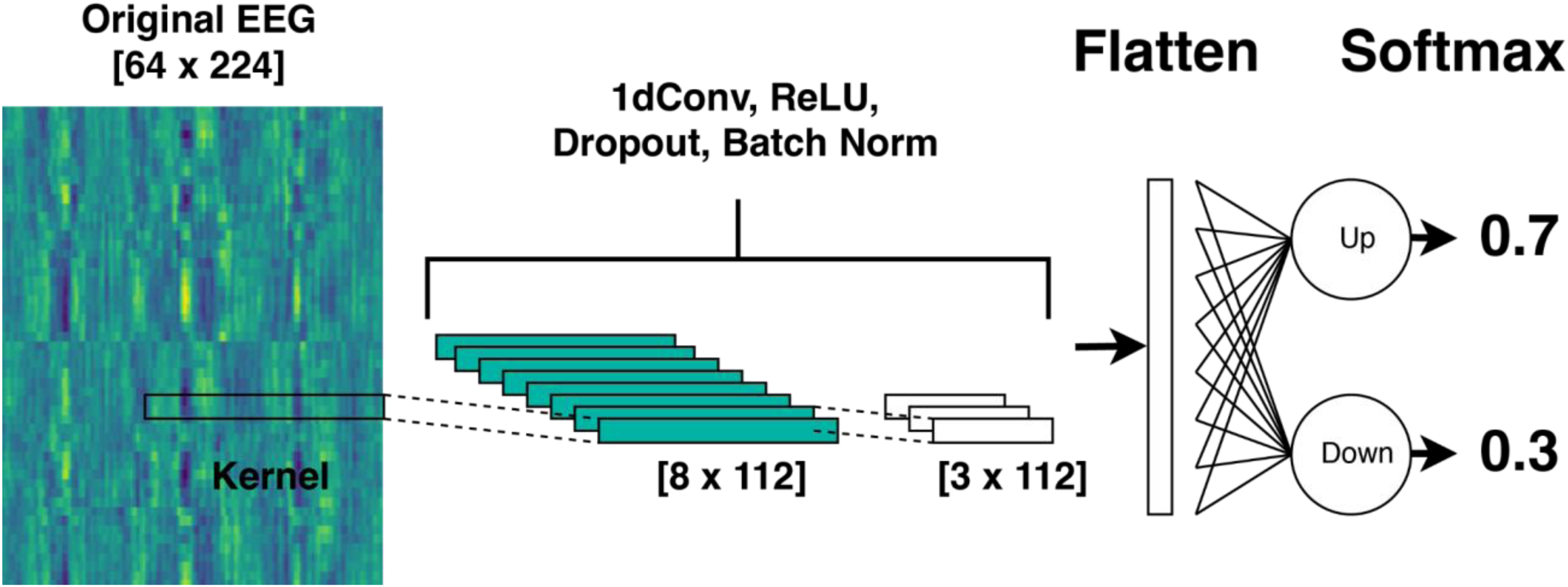
We employed a “mixture of experts,” where multiple individual models’ outputs are combined, enhancing prediction accuracy and robustness (Jacobs et al., 1991). N distinct models received the same input, and their predictions were aggregated by summing their logits. To predict auditory attention, we implemented a mixture-of-experts approach, creating an ensemble of seven models for each test participant. Each participant's ensemble was trained on data excluding that participant's data and the data of an additional five randomly selected participants. Because each subject's EEG measurements differ significantly, building models on subsets of subjects yields models that learn distinct features predictive of auditory attention. Combining their predictions can yield more robust and accurate AAD than a single model trained on all data, by diversifying the training data and reducing susceptibility to individual subsets.

Results

Behavioral Results

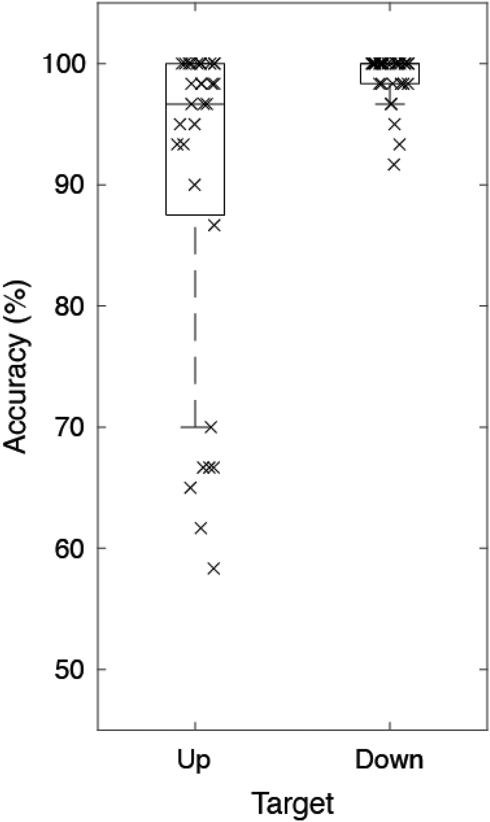
Figure 4 shows participants’ behavioral task performance. The median accuracy was 98.33% (interquartile range [IQR] = 8.13%). The detection accuracy for the target “Up” was 96.67% (IQR = 12.50%) and for the target “Down” it was 100.00% (IQR = 1.67%), which reached the ceiling. Performance for both tasks was above chance level, which was 33.33% for target “Up” and 50% for target “Down.”

OPEN IN VIEWER

Figure 4.

Behavioral task performance. The distribution of behavioral task performance for the “Up” and “Down” targets is presented as a boxplot. The “x”-shaped markers indicate each individual's performance.

Attentional Modulation of Auditory ERP

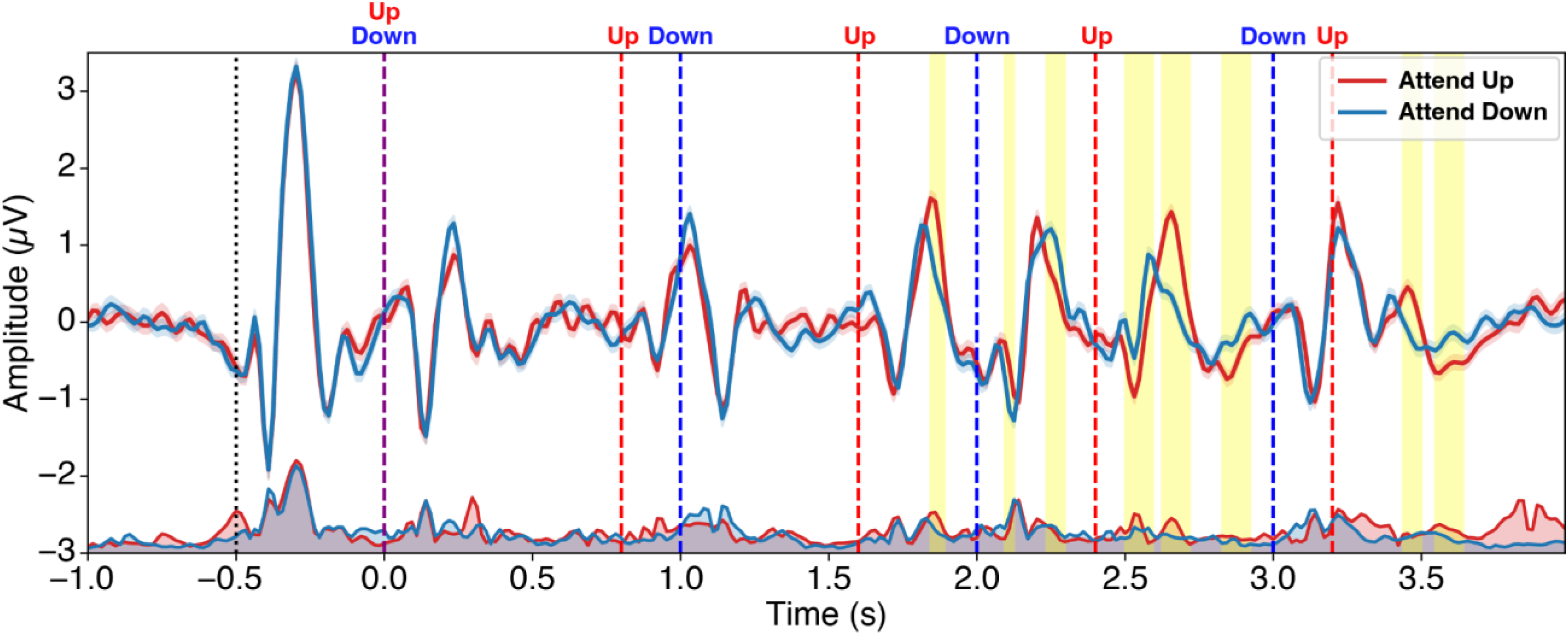
From the grand-average ERP waveform (Figure 5), we were able to observe attentional modulation. The cluster-based permutation test revealed that the P2 response to the third “Up” and the N1-P2 response to the fourth “Up” were larger in amplitude when attended than ignored. Also, N1 response to the third “Down” was larger in amplitude when attended than ignored. The AMI averaged across participants was 0.052 (SD = 0.069), which was significantly greater than zero (one-sample t-test: t = 4.0, p < .001).

OPEN IN VIEWER

Figure 5.

Attentional modulation of the auditory ERPs. The grand-averaged ERP waveform for the “Attend Up” (red) and “Attend Down” (blue) conditions is presented. ERP was derived from the Cz channel. GFP is depicted as a shaded area at the bottom. Yellow-highlighted areas represent temporal clusters of ERP that differ significantly between the “Attend Up” and “Attend Down” conditions. Red dashed lines indicate the onsets of the “Up” sound, and blue dashed lines indicate the onset of the “Down” sound. Black dotted lines at −0.5 s indicate the onset of white noise.

Forward and Backward Linear Modeling

The forward TRF fitted to the attended speech stream, using the same regularization parameter ( λ = 10 4 ), showed similar absolute amplitudes at 100 ms and 150 ms time delays (Figure 6A). When we reconstructed the EEG signal by convolving the fitted forward-model coefficients with the speech envelope, the average correlation coefficient between the actual and reconstructed EEG signals was 0.047 for the attended forward TRF and 0.030 for the ignored TRF, which differed significantly according to a paired t-test (p < .001). Supplemental Figure S2 shows the spatial pattern of correlation coefficients of attended TRF across all channels.

OPEN IN VIEWER

Figure 6.

Attentional modulation modeled with forward and backward linear modeling. (A) Grand-averaged forward TRF coefficients fitted on attended speech stream (green) and ignored speech stream (orange). The x-axis is the time delay, and y-axis is the coefficient value of the fitted TRF. The signals are from the Cz channel. (B) Actual and reconstructed speech envelopes from a fitted backward linear model. The black line is the actual envelope, and the red and blue lines are the reconstructed envelopes for each target “Up” and “Down.” Solid lines are reconstructed from the attended backward linear model, dashed lines are reconstructed from the ignored backward model. The shade indicates the standard error among participants. Note that the amplitude of the reconstructed signal was scaled up for visualization.

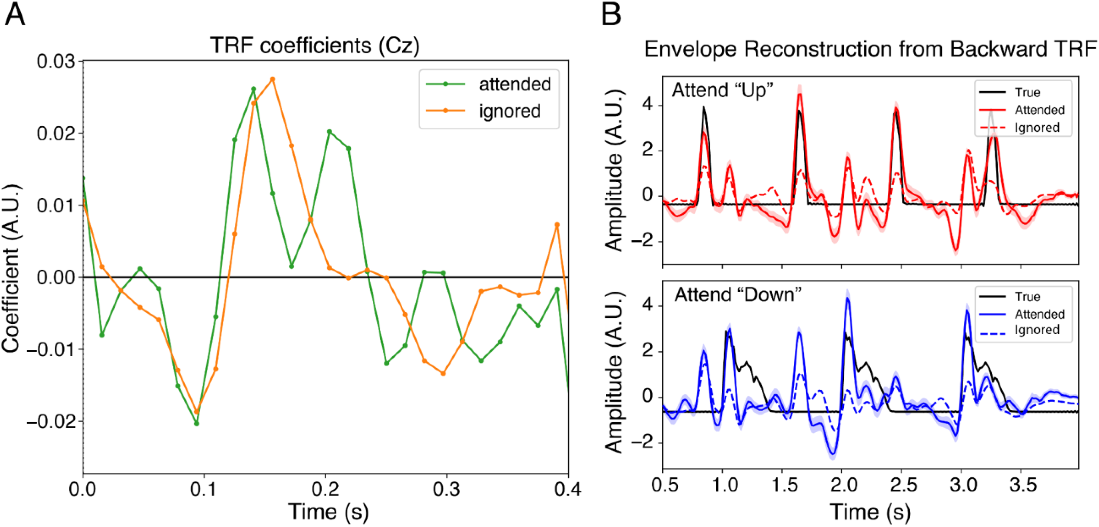
The speech envelopes were reconstructed for each trial by convolving the fitted backward model with the single-trial EEG signal. Figure 6B shows the waveform of the actual speech envelope and the reconstructed speech envelope averaged across trials and participants for each attentional target. The reconstructed speech envelope from attended TRF aligns better with the peaks of the envelope than the reconstructed envelope from ignored TRF. The correlation coefficient between the reconstructed speech envelope from the attended backward linear model and the real signal was 0.20 (SD = 0.00046), and the correlation with the ignored backward linear model was 0.081 (SD = 0.0013), which was significantly lower (p < .001).

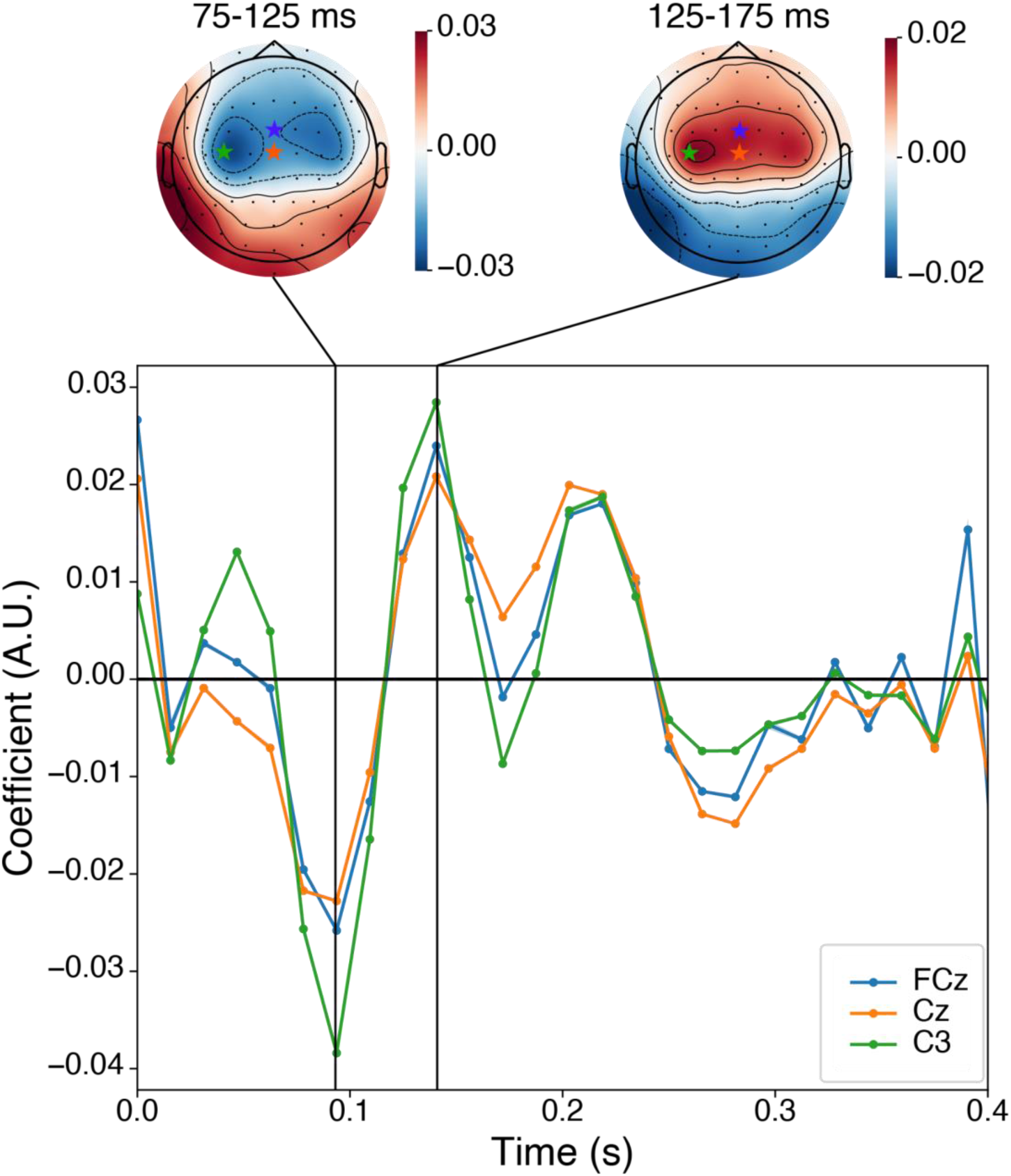
Figure 7 shows the coefficients of the fitted forward model. The waveform from the frontocentral channels (FCz, Cz, and C3) was similar to the typical auditory ERP of the P1-N1-P2 complex, but with a shorter latency. The topography of TRF coefficients at 100 ms and 150 ms (corresponding to N1 and P2) was also similar to that of the auditory ERP; it showed a bipolar distribution centered on the central and temporal regions.

OPEN IN VIEWER

Figure 7.

Temporal response function from the fitted forward model. A topography and time course of TRF coefficients across time delays. The time course was drawn from channels FCz, Cz, and C3. C3 had the largest peak value. The coefficients were averaged across all outer cross-validation folds.

For the following attention-decoding analysis, we used only the attended TRF, which was fitted using the target speech envelope for each trial. Our current decoding framework relies on correlations between predicted and actual EEG signals to determine attentional focus. Specifically, we apply the attended TRF to each of the two possible speech streams (“Up” vs. “Down”) to generate competing EEG predictions. Because the prediction step already contrasts the two streams, the decoder implicitly incorporates the differential representation of attended and ignored speech.

Attention Decoding Performance

Figure 8 shows the accuracy of auditory selective-attention decoding across the decoders we compared. All the decoders yielded performance significantly above the chance level at the group level. The average decoding accuracy was highest with the CNN decoder (72.3 ± 9.1%), while the forward TRF decoder with logistic regression (64.9 ± 6.5%), with SVC (64.1 ± 6.5%), and the backward linear model decoder (64.9 ± 8.9%) showed comparable performance. Decoding performance differed significantly among decoders (p = .006). As shown in Table 1, the post-hoc Wilcoxon test revealed that the CNN decoder performed significantly better than all other decoders by around 5% points in accuracy. There was no significant difference in performance between logistic regression, SVC, and the backward model decoder.

OPEN IN VIEWER

Figure 8.

Decoding performance of different attention decoders. Decoding performance was evaluated by leave-one-subject-out cross-validation. Each point represents performance from a single cross-validation fold, evaluated on data from a single test participant. The performance was highest with the CNN decoder, while the forward TRF decoder with logistic regression, SVC, and the backward linear model decoder showed comparable performance.

OPEN IN VIEWER

Table 1.

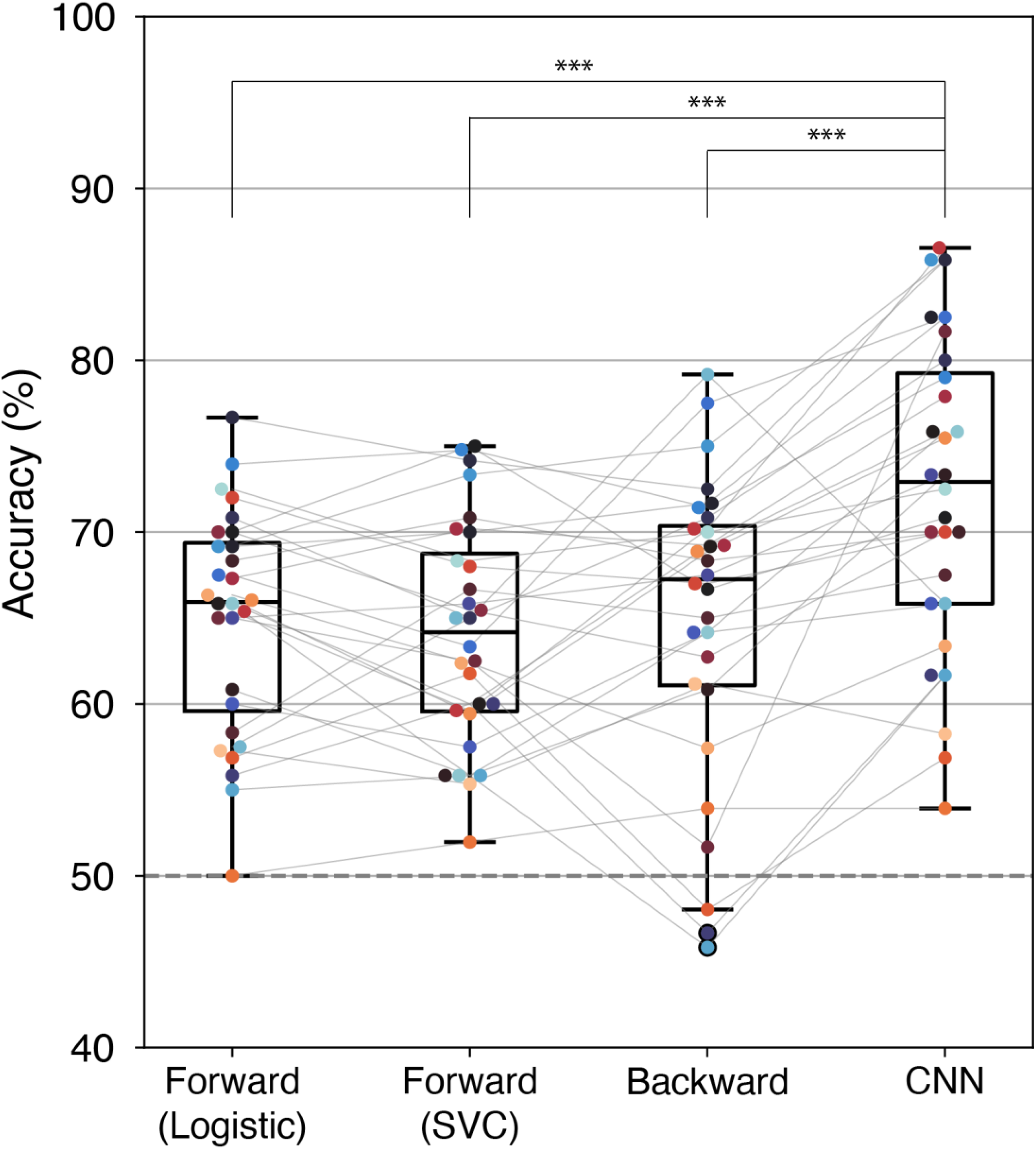
Differences in Decoding Accuracy Across Decoders.

Test	Decoder 1	Decoder 2	Difference in Accuracy	p-Value	p-Value (Bonferroni)
Wilcoxon	CNN	Backward	+7.4%	<.001	<.001
Wilcoxon	CNN	SVC	+8.2%	<.001	<.001
Wilcoxon	CNN	Logistic regression	+7.4%	<.001	<.001
Wilcoxon	Backward	SVC	+0.8%	.516	1.000
Wilcoxon	Backward	Logistic regression	0%	.819	1.000
Wilcoxon	Logistic regression	SVC	+0.8%	0.311	1.000

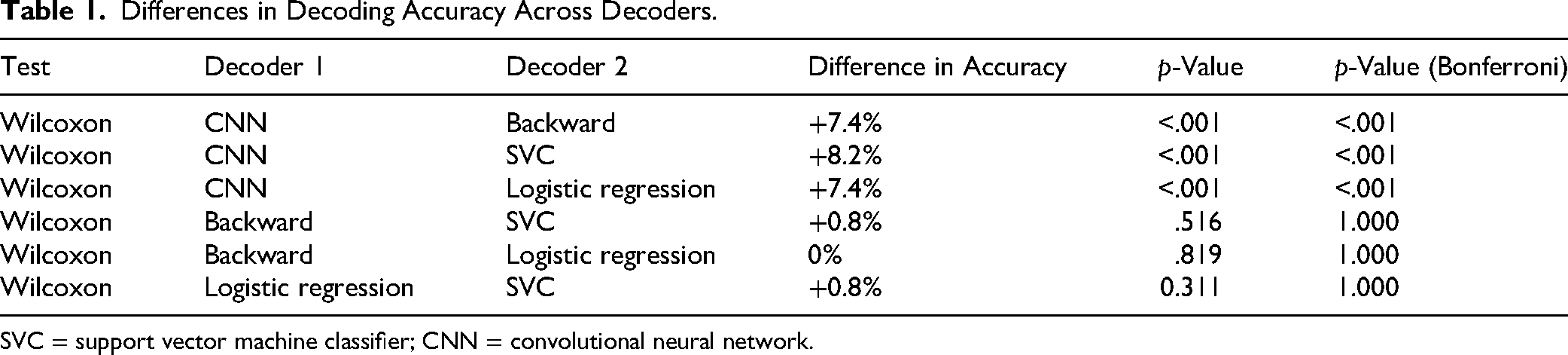
SVC = support vector machine classifier; CNN = convolutional neural network.

Decoding performance varied depending on which participant's data was used as a test set. This variability was not correlated with an individual's AMI (Figure 9, top row). The accuracies of different decoders were correlated with one another, except for the SVC-CNN pair (Figure 9). The decoder using the forward linear model—Logistic regression and SVC—had the highest correlation ( ρ  = 0.75), which was consistent with the high Kappa agreement between the two (see Supplemental Table S1).

OPEN IN VIEWER

Figure 9.

Correlation of AMI and decoding accuracies and between decoder pairs. The top row shows the correlation between AMI and decoding accuracy in the ratio unit. The second through fourth rows show the correlations for each decoder pair. Dots indicate data points from each left-out test participant. Trend lines are shown in red, with confidence intervals shaded. Spearman correlation coefficient ( ρ ) is noted in each panel. Significance of the correlation was corrected for multiple comparisons using the Bonferroni method (*: p < .05, **: p < .01, ***: p < .001.

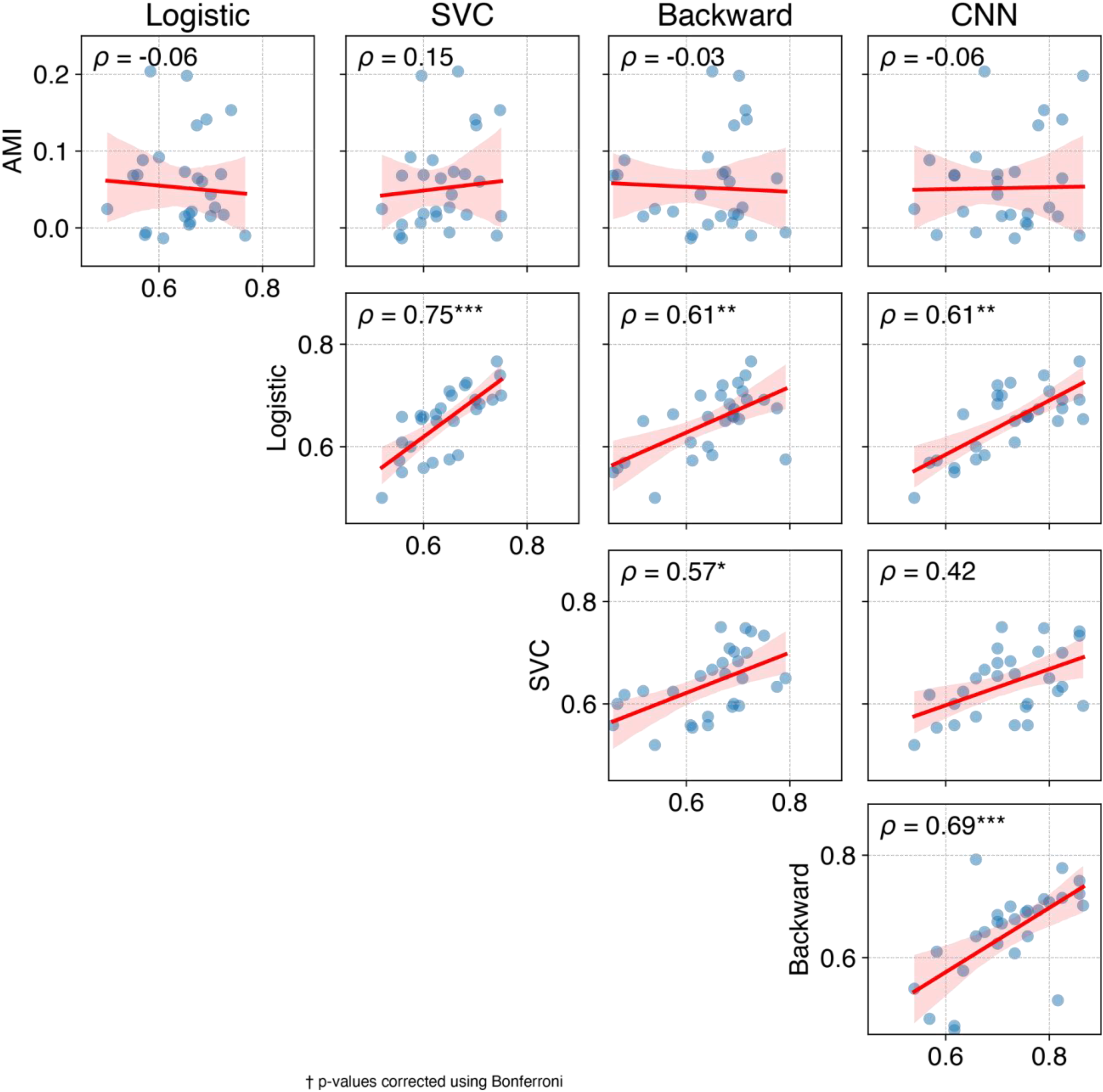
Temporal and Spatial Pattern of Associations Between Attentional Modulation and Attention Decoding

Temporal Patterns of Associations

Our hypothesis was that if the attentional modulation (i.e., the amplitude of the neural response to the same sound is larger when it is attended than when it is ignored) is more prominent in the correctly classified trials than the incorrectly classified trials, we can infer that the decoder, at least partially, was relying on the attentional modulation.

Cluster-based permutation tests (p < .05) revealed that attentional modulation was observed more frequently in correctly than in incorrectly classified trials across all four types of decoders (Figure 10).

OPEN IN VIEWER

Figure 10.

Reflection of attentional modulation in the attention decoding. ERP and global field power (GFP) from correctly versus incorrectly classified trials are presented for all four decoders. For each pair of panels, the top panel corresponds to ERPs from correctly classified trials, and the bottom panel corresponds to ERPs from incorrectly classified trials. Red lines show the grand-average ERP for “Attend Up” trials, and blue lines for “Attend Down” trials. Shaded areas represent the standard error across participants. All results are from the Cz channel. The ERP is plotted in the main panels, while GFP is plotted at the bottom of each panel. Yellow-highlighted areas represent temporal clusters that differ significantly between the “Attend Up” and “Attend Down” conditions. Dashed lines indicate onsets of the sounds. The color of these lines corresponds to the stimulus type: gray for the white noise, red for “Up” speech, and blue for “Down” speech. The waveform of the sound stimuli is depicted in the middle of each column for reference.

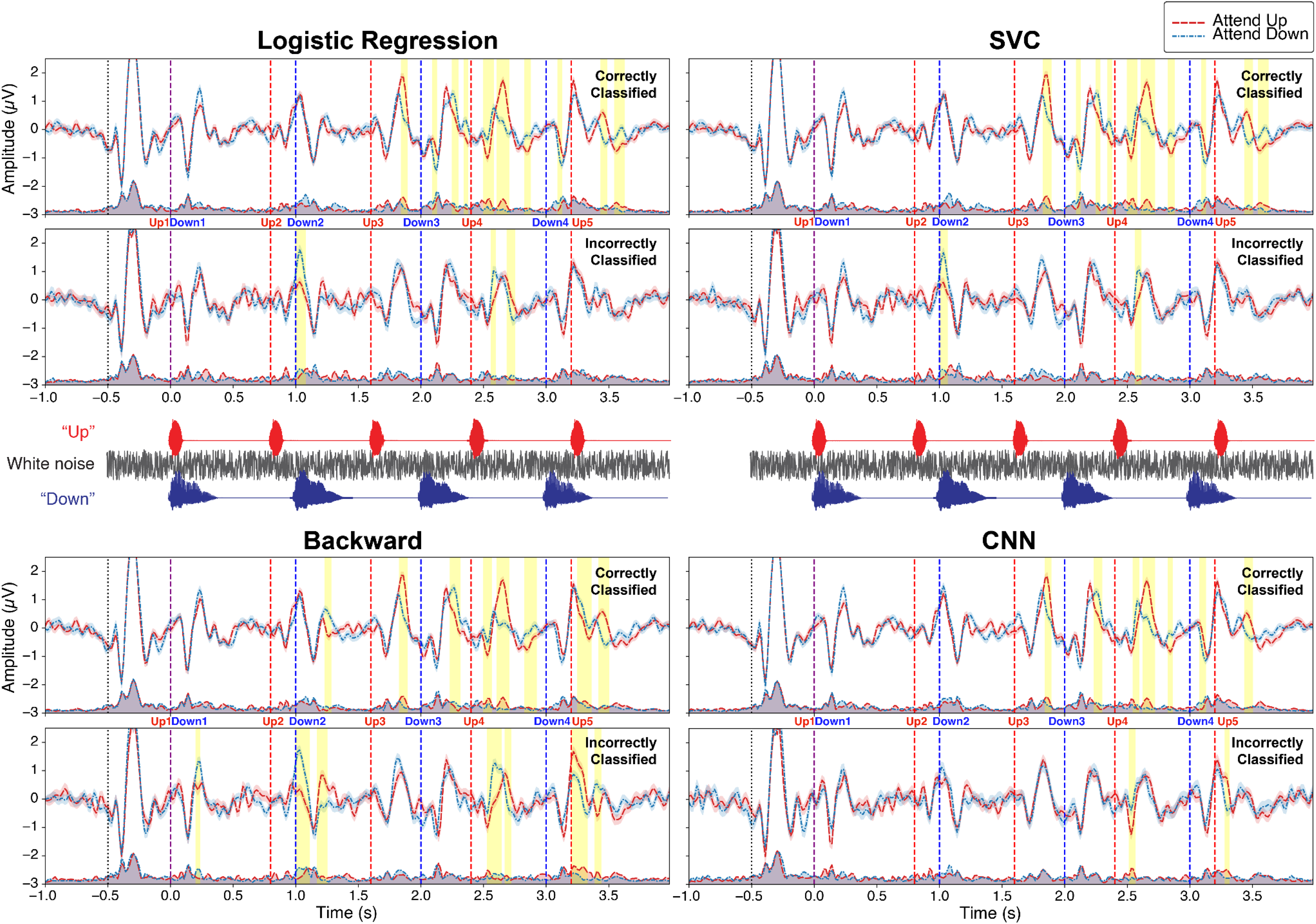
We labeled the cluster corresponding to the N1-P2 response to each word onset, combining the speech type (“Up” or “Down”), word position (2, 3, 4, or 5), and ERP peak type (P1, N1, or P2). For example, the N1 response to the third “Up” sound is labeled as Up3-N1. Clusters after the P2 peak were not included in further analysis since we focused on the attentional modulation of N1-P2 peaks.

Overall, there were a total of eleven significant clusters to investigate: Up2-P2, Down2-P2, Up3-P2, Down3-N1, Down3-P2, Up4-N1, Up4-P2, Down4-N1, Down4-P2, Up5-N1, and Up5-P2. Among these clusters, Up2-P2 and Down4-P2 were excluded since the timing overlaps with Down2-P1 and Up5-P1, respectively, and were unable to dissociate the impact of the attentional modulation on the amplitude change of each component. Therefore, nine clusters were further investigated.

The correctly classified trials of logistic regression and SVC decoders showed six significant attentional modulation clusters: Up3-P2, Down3-N1, Up4-N1, Up4-P2, Down4-N1, and Up5-P2. The correctly classified trials of the backward model decoder showed six significant attentional modulation clusters: Down2-P2, Up3-P2, Up4-N1, Up4-P2, Up5-N1, and Up5-P2. Among these clusters, Up4-N1 was also observed in trials that were incorrectly classified. The correctly classified trials of the CNN decoder showed six significant attentional modulation clusters: Up3-P2, Down3-P2, Up4-N1, Up4-P2, Down4-N1, and Up5-P2. The Up4-N1 cluster was also observed in trials that were incorrectly classified.

It is worth noting that, based on the backward model decoder results, Down2-P2, Up4-P2, and Up5-P2 showed attentional modulation in the opposite direction, with the response to the sound when it was a target being smaller than when it was not.

In summary, the total number of clusters that matched the hypothesis was six across all four decoders. For the backward model decoder and the CNN decoder, one cluster (Up4-N1) was identified in both correct and incorrect trials, contrary to the hypothesis.

Figure 11 shows the AMI distribution across participants for correctly and incorrectly classified trials for each decoder. For the two forward linear model decoders (logistic regression and SVC), the AMI of incorrectly classified trials was significantly lower than the AMI of correctly classified trials (logistic regression: p < .05, SVC: p < .001); the backward linear model decoder and CNN decoder did not show such a difference (p > .5).

OPEN IN VIEWER

Figure 11.

Difference of AMI between correctly and incorrectly classified trials. The boxplot with scatter points shows the distribution of AMI values across participants. The AMI for a test participant excluded from the analysis was calculated separately for correctly and incorrectly classified trials. Significance of difference between the two distributions is marked with asterisks (*: p < .05, **: p < .01, ***: p < .001, n.s.: p > .05).

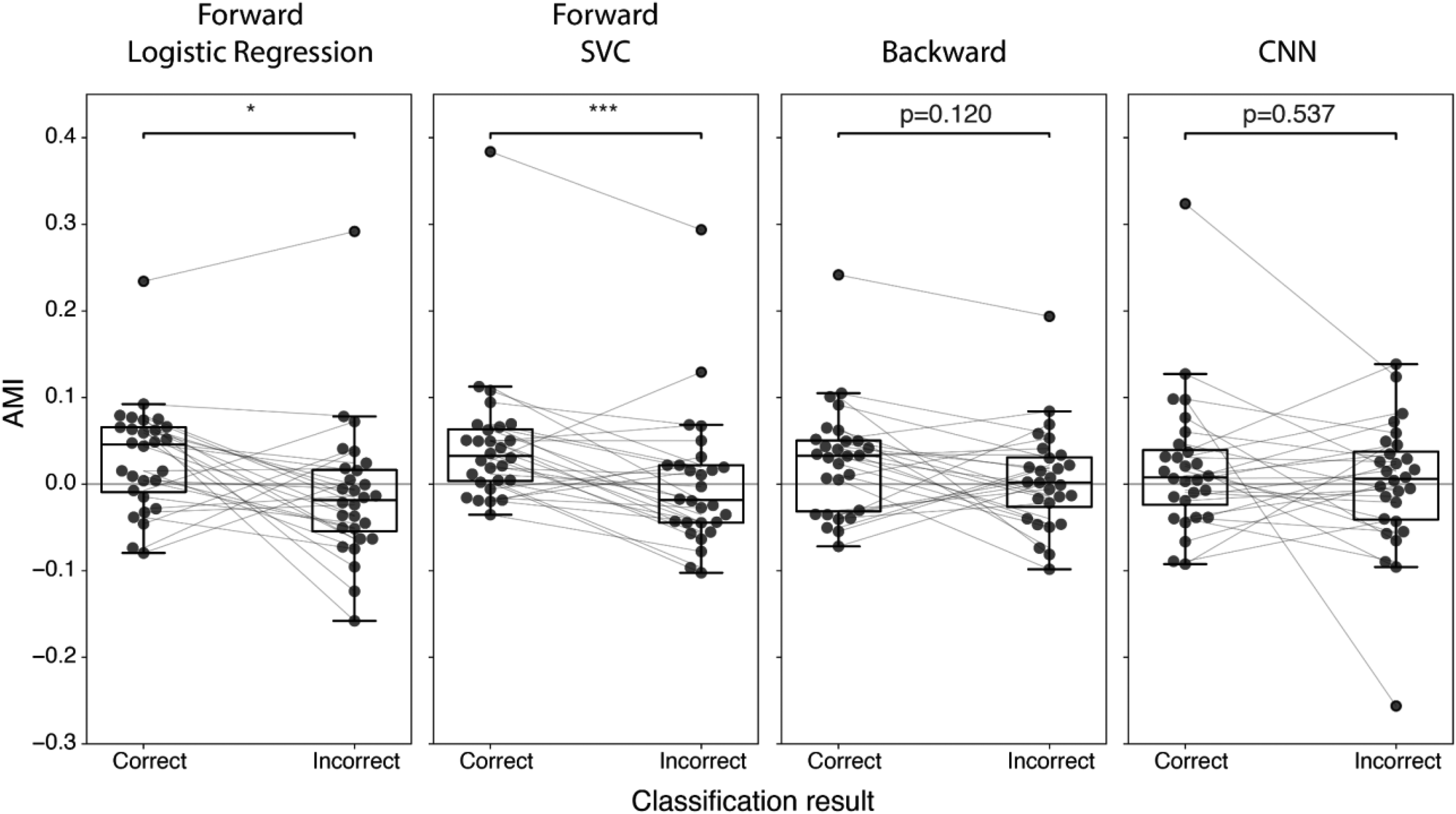
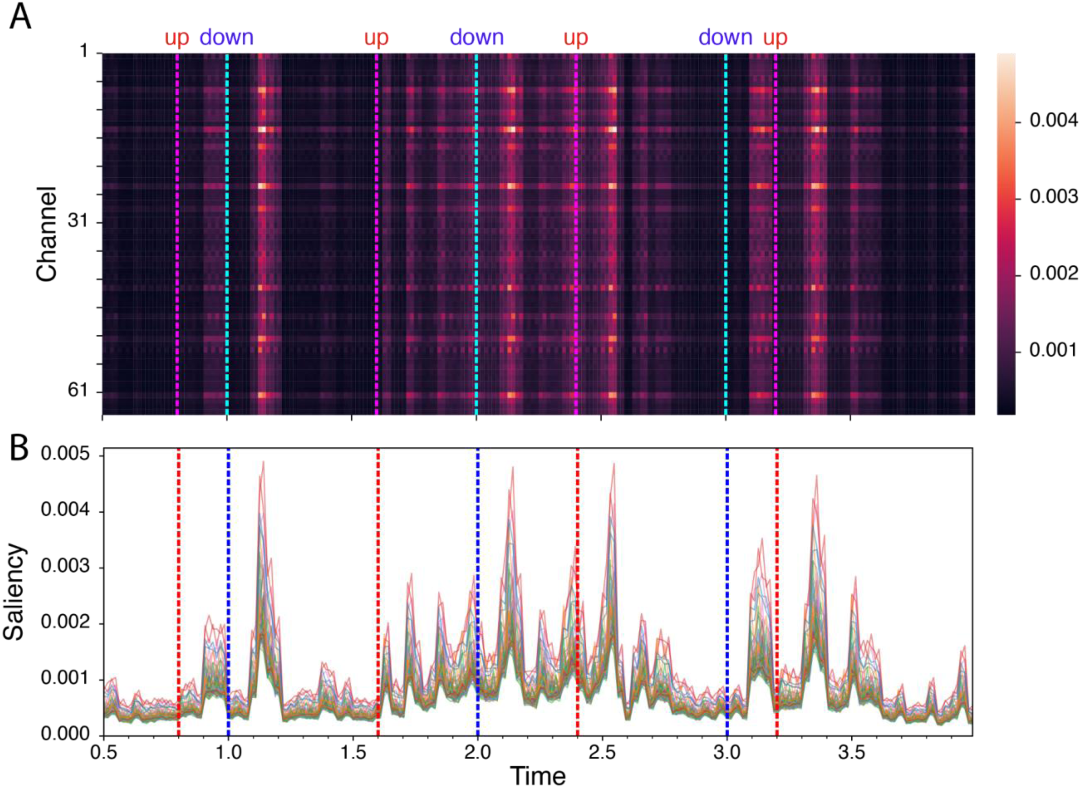
Figure 12 shows the spatio-temporal pattern of saliency from the CNN decoder. The temporal pattern is discussed here first; the spatial pattern is discussed in the next section with Figure 13. We can observe the temporal windows with large spatial variance peaks around 100–200 ms and 200–300 ms after each onset of speech. These peak saliency latencies aligned with the traditional N1-P2 response window relative to the sound onset. The salient time windows largely aligned with the clusters identified from grand-averaged ERPs (Figure 5), and correct versus incorrect comparisons (Figure 10), except for the Up5-P2 response, which did not appear in the salience map. EEG signals from N1-related time windows were more salient for model performance than the signals from P2-related time windows.

OPEN IN VIEWER

Figure 12.

Saliency map of the CNN decoder. (A) Saliency map of the CNN decoder across time and channels. Brighter colors indicate higher importance. Onsets of sound “Up” and “Down” are indicated by a vertical dotted line (Up: magenta, Down: cyan). (B) Temporal importance is illustrated by the saliency waveform over time. Onsets of sound “Up” and “Down” are indicated by a vertical dotted line (Up: red, Down: blue).

OPEN IN VIEWER

Figure 13.

Spatial pattern of the EEG features associated with the attention decoding derived from three different decoder models. The spatial contribution of EEG features to attention-decoding decisions is analyzed separately for each decoder type. (A) The activation patterns of the forward model decoder were calculated by correlating the input features (channel-wise EEG reconstruction correlations) with the decoder decision values (logits) across all test trials. The left topography shows the correlation coefficients computed from the predicted EEG using the “Up” envelope; the right topography shows the decoder weights for the correlation coefficients computed from the predicted EEG using the “Down” envelope. Note that the two topographies (“Up” and “Down”) share a colorbar because they were derived from a single classifier. (B) The activation patterns of the backward model across different time windows. Time delays corresponding to the N1, P2, and P3-related windows were selected. (C) The saliency topography of the CNN decoder is aggregated from the spatiotemporal salience map by taking the RMS of the whole time window.

Spatial Patterns of Associations

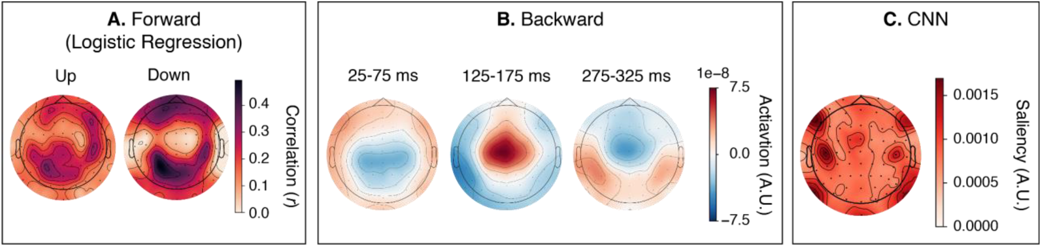
Figure 13 shows spatial patterns associated with attention decoding, estimated separately for each decoder type (see the methods section for details).

The activation pattern of the forward logistic regression model (Figure 13A) showed high correlations distributed across central and parietal electrodes. The patterns for “Up” and “Down” are similar, with “Down” showing more contrast. The activation pattern of the backward linear model (Figure 13B) indicates that decoding is associated with distinct temporal stages rather than maintaining a static topography. The early processing window (25–75 ms) was characterized by a negative-polarity distribution over central sensors. This was followed by a polarity reversal in the 125–175 ms window, where a robust positive activation pattern emerged with a fronto-central topography. A second polarity reversal occurred in the late latency window (275–325 ms), returning to a negative fronto-central pattern. The CNN model's saliency map (Figure 13C) also showed sensitivity to central regions. However, its spatial pattern featured focal, high-saliency clusters over bilateral temporal and parietal areas.

Discussion

In this study, we examined how various AAD models perform on 4-s colocated speech streams and how these decoder models align with established ERP-based measures of attentional modulation. We found that the CNN decoder achieves approximately 72%, whereas the linear-model-based decoders achieve approximately 65%. The number of N1-P2 peaks that were significantly larger when attended than ignored was higher in correctly decoded trials than in incorrectly decoded trials. Individual variance of N1 peak-based AMI was not correlated with the decoder's performance. The difference of AMI calculated from the correctly decoded trials versus incorrectly decoded trials was significant only in the forward linear model-based decoders, but not in the backward linear model decoder and CNN decoder.

Regardless of having no spatial separation during sound presentations, the performance of our decoders is broadly consistent with previous AAD algorithms, including those with deep learning approaches (Cai, Schultz, & Li, 2024; Mahjoory et al., 2024; Nguyen et al., 2025; Su et al., 2022; Tian & Ma, 2020; Vandecappelle et al., 2021). Recently reported performance of subject-independent decoder on spatially separated AAD datasets for 5-s-long decision windows is around 60–65% with the backward model and 65–70% CNN (Nguyen et al., 2025). This suggests that effective attention decoding is achievable even in the more demanding colocated condition.

The superior performance of the CNN decoder over linear model-based decoders is consistent with previous studies showing that deep neural networks can decode selective attention from EEG within a time window of 5 s or less (Mahjoory et al., 2024; Su et al., 2022; Tian & Ma, 2020). Our results extend these findings by demonstrating that CNNs maintain this advantage even when stimuli are spatially colocated.

Multiple factors may have contributed to the CNN model's superior decoding performance relative to linear models. From the temporal association to the attentional modulation of ERP and the time series of the saliency, we could infer that the CNN model was mostly relying on the 100–300 ms latency window after the onset of each word. Although the backward model decoder appears to use information from a time window, the CNN still performs better. Given that neural networks can capture subtle, nonlinear spatiotemporal patterns in neural signals, the CNN decoder may have detected faint task-related features embedded in noisy single-trial EEG (Rakhmatulin et al., 2024). In our case, CNNs learned multiple nonlinear kernels that abstract information from the entire EEG sequence, rather than using a single fixed kernel with a time-lagged linear function. Additionally, the “Mixture of Experts” strategy, which used an ensemble of multiple models trained on different subsets of data, could have contributed to a better performance. However, these interpretations stay hypothetical without ablation testing that systematically removes identified ERP clusters and measures resulting loss in accuracy, which remains for future work.

There was significant variability in decoding accuracy across different participant data sets used as test sets. Because behavioral performance was at or near ceiling for most participants, we could not examine whether individual selective attention performance was associated with this variance. Partial fine-tuning using a small subset of individual data may enhance performance without compromising generalization (Beauchene et al., 2023; Tian & Ma, 2020) and should be explored in the future.

All four models showed links to established neural markers of selective attention. For all four decoders, we found five to six time clusters that showed significant attentional modulation of auditory ERPs (larger amplitude to the target onset when attended) averaged from trials that are correctly classified by the decoders (Figure 10). The number of significant clusters was smaller or none for ERPs averaged from the incorrectly classified trials. These clusters overlapped with clusters found from grand-averaged ERPs (Figure 5), indicating that attention decoding was predominantly based on attentional modulation of N1-P2 responses to the sound onsets.

In contrast, the AMI calculated from the N1 peak of GFP was higher in the correctly classified trials than in the incorrectly classified trials only for the forward linear model decoders. Three out of six attentional modulation clusters were N1-related in the forward linear model results, while two out of six were N1-related and one N1 cluster was also found from incorrectly classified trials in backward and CNN. This might indicate that the forward linear models relied more on N1-related attentional modulation, whereas backward and CNN decoder relied on time windows spanning across N1-P2 responses or were influenced by other unexplained variance. Consistent with this, the reverse pattern of P2-related attentional modulation in incorrectly classified trials was observed in backward model-based decoder results. The saliency map of the CNN decoder shows peaks around 100–300 ms after almost every speech onsets, which might indicate that the model is exploiting both attention-dependent modulation and subtle single-trial variability that cannot be captured in group-level statistics. However, to identify the cause of this discrepancy, further investigations are required in the future such as ablation study that shows decrease in decoding performance after removing specific time windows.

Despite differences in AMI between correctly and incorrectly classified trials, we found no correlation between participants’ N1-based AMI and classifier decoding accuracy. Given that all participants performed well on the behavioral task, the variability in selective attention ability might have been small. Assuming small variance among participants, decoding accuracy may be driven more by trial-to-trial fluctuations than by stable differences in attentional modulation. Two analysis differences further decouple AMI and decoding: (a) decoding is computed on single trials, whereas AMI is computed from condition-averaged metrics, making AMI less sensitive to unsystematic trial-level variability; and (b) decoding uses a broad 0–0.4 s window, whereas AMI in our implementation is N1-specific. Given these differences in estimation level and time window, a strong between-participant correlation between AMI and decoding accuracy is not necessarily expected. It is also worth noting that we could not determine whether the decrease in AMI from incorrectly classified trials is due to weaker attentional modulation or to noise in the single-trial EEG.

The spatial patterns of the EEG features associated with attention decoding were distinct across decoder types. In the forward model, a topographic pattern centered on the parietal and central regions was observed for the “Up” and “Down” labels. This suggests that the decoder learned a stable spatial pattern. However, because the forward model collapses temporal information into a single correlation value, we can only capture the overall spatial pattern, not the dynamics. For the backward linear model, however, we observed a spatiotemporal pattern that resembles auditory evoked potentials. Polarity flipping was observed across different time windows, indicating that the backward linear model decoder learned dynamic encoding of attention-related neural responses. The CNN decoder exhibited a focal salience map, consistent with that of a simpler neural network model (de Taillez et al., 2020). This suggests that the CNN learned spatially meaningful features from the EEG time-series input. However, because the spatial feature importance was assessed qualitatively, additional analyses, such as permutation feature importance (Altmann et al., 2010), could further substantiate the significance of each channel for attention decoding. Additionally, because the method for calculating spatial patterns differed across decoders, direct comparisons of spatial patterns across decoder types should be interpreted cautiously.

Although spatial cues are central to auditory selective attention in everyday environments, we deliberately used colocated streams in this study. This choice reduces ecological validity, and we explicitly acknowledge that our paradigm does not capture spatial-selective mechanisms such as hemispheric lateralization of cortical oscillations (e.g., Deng et al., 2019; Kerlin et al., 2010; Wöstmann et al., 2021). However, many EEG-based selective-attention paradigms employ fixed spatial configurations with static binaural cues, despite the fact that real-world listening involves continuous head movements that dynamically change interaural timing and level differences. Several AAD models are known to rely heavily on such hemispheric lateralization patterns induced by fixed spatial cues (Cai, Schultz, & Li, 2024; Mahjoory et al., 2024; Vandecappelle et al., 2021). Decoders that rely on these fixed spatial patterns may generalize poorly to natural scenes in which the listener moves and spatial configurations vary. By removing spatial cues, our design emphasizes temporal and spectro-temporal attentional markers (i.e., features that remain stable when listeners turn their heads) and reduces the likelihood that decoding relies on fixed spatial patterns. However, we did not explicitly test whether the current models in this colocated setting generalize to scenes with spatial separation. Spatial cues remain important in real-world listening, and our approach should be viewed as a complementary paradigm for understanding model behavior when spatial information is absent. Future work should directly quantify cross-condition generalization by training and testing decoders across colocated, spatialized, and dynamically shifting spatial configurations.

It is worth noting that the use of repetitive stimuli across trials is a double-edged sword; it allows straightforward analysis and interpretation of attentional modulation with minimal confounds, but at the cost of limited ecological realism. Additionally, repetitive stimuli might have limited the decoder's ability to learn stimulus-invariant neural patterns. Because each stimulus had the same structure, the decoders may have partially relied on trial-specific regularities. Future studies should test whether these decoders generalize to novel audio materials or sentence structures.

Conclusion

By using a two-stream, colocated listening paradigm with a fixed, highly regular temporal structure, we demonstrated that the basis of attention decoding from auditory stimuli can be tested by aligning model output with ERP and AMI. Forward linear model, backward linear model, and CNN decoders all showed alignment to the known attentional modulation of ERPs, while the forward model exhibited a more pronounced association with N1-peak-related alignment. The CNN model showed superior decoding performance compared with other models, partially due to its capacity to encode nonlinear information on top of known ERP-related features. These findings lay the mechanistic baseline for interpreting EEG-based attention decoding in terms of classic neural indices and provide a principled framework for evaluating new AAD approaches in paradigms designed to expose attentional modulation with minimal confounds.

Supplemental Material

Supplemental Material

Supplemental Material

Supplemental Material