Land use change simulation and analysis using a vector cellular automata (CA) model: A case study of Ipswich City,Queensland,Australia

Abstract

The loss of accuracy in vector-raster conversion has always been an issue for land use change models, particularly for raster based Cellular Automata models. Here we describe a vector-based cellular automata (CA) model that uses land parcels as the basic unit of analysis, and compare its results with a raster CA model. Transition rules are calibrated using an artificial neural network (ANN) and historical land use data. Using Ipswich City in Queensland, Australia as the study area, the simulation results show that the vector and raster CA models achieve 96.64% and 93.88% producer’s spatial accuracy, respectively. In addition, the vector CA model achieves a higher kappa coefficient and more consistent frequency of misclassification, while also having faster processing times. Consequently, the vector-based CA model can be applied to explore regulations of land use transformation in urban growth process, and provide a better understanding of likely urban growth to inform city planners.

Keywords

Land use change vector-based cellular automata urban growth artificial neural network Ipswich City

Introduction

Land use change modelling, as an aid to understanding city changes, has been the subject of research for more than 30 years (Batty and Xie, 1994; Clarke et al., 1997; Couclelis, 1989). The theory and application of these models have been a key topic of research in GIS, and they are important tools for the analysis of land use dynamics (Verburg et al., 2004a). Cities have been identified as complex systems with dynamic and nonlinear characteristics, and the regulations of land use evolution can be determined from cities with the help of land use change models (Batty, 2009; Yang et al., 2016). Additionally, the dynamics of potential future development of study regions can be achieved, leading to new insights of further analysis of the land-use change process under various scenarios (Shahumyan and Moeckel, 2017; Yang et al., 2018).

There are many types of land use change models, including Agent-based models (ABM) (Li and Liu, 2008; Long and Zhang, 2015), Cellular Automata (CA) (Almeida et al., 2008; Li and Yeh, 2002a), Conversion of Land Use and its Effects (CLUE) (Verburg and Veldkamp, 2001), and What if? (Klosterman and Pettit, 2005; Pettit, 2005). Among these, CA models have been applied in the field of land use change and urban development (Feng and Tong, 2018b; Liu et al., 2008; Verburg et al., 2004b), and derived new models such as SLEUTH (Jantz et al., 2004; Mahiny and Clarke, 2012) and FLUS (Liang et al., 2018; Liu et al., 2017). These models are designed to analyse the relationship between driving forces and land use change, and predict its future development. In general, CA is considered a bottom up urban model from which emergent patterns of land use change arise as derived from ‘simple’ transition rules, which is in accordance with the essence of complexity science: a complex system is derived from the interactions of simple subsystems (Li et al., 2007).

Generally speaking, a CA model consists of four components (online supplementary Figure S1): cells, cell space, transition rules and the neighbourhood configuration (Li et al., 2007). A cell is the basic unit of the model, and represents some part of the real world. The cell space comprises the set of cells in the model, and spans the extent of the study area. Transition rules are of key importance in CA since they determine whether the state of a cell will be transformed at a time step. These rules can be described by a set of functions, and in most cases are the combination of driving factors, neighbourhood influences, constraints for sustainable development of the study area, as well as random disruption (Liu et al., 2010; White et al., 1997). The neighbourhood configuration defines the surrounding environment around a cell that influences it.

Transition rules are a significant component of CA models (Li et al., 2007), and many different methods have been used to calibrate them. There is not yet consensus about which is the ‘best’ approach, but primarily, it is possible to obtain more accurate transition rules using artificial intelligence techniques than traditional techniques (Li et al., 2010).

While progress has been made on transition rules, the choice of data format is an active area of research, specifically raster versus vector. The raster data format is still most commonly used (Liu, 2008), partly because land use data are commonly derived from satellite images, and also because the simple data structure leads to simpler algorithms. However, there are several issues with the use of raster data for modelling geographic objects in land use change models. First, the size of a raster cell has a considerable impact on simulation dynamics in terms of both land-cover area and spatial structure (Ménard and Marceau, 2005). Second, the fixed neighbourhood configuration of raster CA inhibits their ability to accurately simulate geographical processes – urban space transformations rarely follow regular geometric patterns (Barreira-González et al., 2015). Third, land parcels and not grid cells are the elemental unit of planning instruments such as planning zones and urban growth boundaries. Planning support systems such as What if? and CommunityViz (Geertman et al., 2013; Pettit et al., 2015) typically are built upon vector data models, so they can precisely incorporate such planning instruments into their models.

The use of vector data for CA modelling is a topic of research that is receiving increasing attention. Initial research used Voronoi diagrams with randomly distributed cells (Flache and Hegselmann, 2001), while O’Sullivan (2001) proposed a graph-CA to define the cell space by vertices and edges. However, as with raster-based models, these approaches are limited by the mismatch between the data format used and the phenomenon being modelled. As a result, cadastral land parcels have been widely used for the definition of cells in vector CA. In the past decade, the VecGCA, DLPS-VCA and MUGICA models have been developed at the cadastral land parcel scale, with globally-distributed study regions in Canada (Southwest Alberta), China (Shenzhen City) and Spain (Madrid region) (Barreira-González et al., 2017; Moreno et al., 2009; Yao et al., 2017). Generally speaking, for the purposes of land use modelling, land parcels are a better representation of the real world than raster cells (Long and Wu, 2017).

However, most of the aforementioned research focuses on the definition of vector cells and transition rules. The relationship between simulation results and sampling strategy for the calibration data has not been fully analysed. In addition, there is still a paucity of research on vector CA in areas experiencing rapid urbanization such as many parts of the world including Australia, China, India and the United States.

Consequently, the overall objective of this study is to assess the performance of CA models using different data formats. The specific question addressed is whether vector CA are more accurate than raster CA for modelling land use changes in cities experiencing rapid growth. Both vector and raster CA models are implemented to simulate land use changes over a 17-year period for a study area in Queensland, Australia.

This paper is divided into three sections following this introduction. In the section Structure of CA models, methods of calibrating and validating transition rules, and the main analysis workflow are illustrated in more detail. Next, the driving factors and the simulation experiments of the study area are described. Finally, the simulation results and key findings of this work are analysed and discussed.

Structure of CA models

The differences between vector and raster CAs

As noted above, the fundamental difference between vector and raster CAs is the smallest unit of analysis, with the cells being modelled as either square (raster) or irregular polygons (vector). This leads to differences in the neighbourhood configuration between the two types of model. For both models, there are two primary types of cells: centre and neighbour. The state of centre cell at an iteration is a function of the values of itself and its neighbours (Lu et al., 2015). In raster CA, Von Neumann and Moore neighbours are most commonly used, in which the neighbouring cells are typically assigned equal or similar weights. However, with respect to vector CA the diversity of polygon shapes means that the connections between neighbouring cells differ and thus there are differing impacts on the transformation probability of a centre cell. For example, a centre polygon might share a long boundary with one adjacent polygon, and thus there is a high potential interaction, and only a very short boundary with another and thus a lower interaction potential. In this work we define vector neighbours as those intersecting a buffer surrounding the central cell.

Generally speaking, the influence a centre cell obtains is a function of the areas of the neighbour cells (polygons) that are within the neighbourhood. As Figure 1 illustrates, neighbour cell N1 has a higher influence on the centre cell than other neighbour cells due to the centroid distance between itself and the centre cell. In addition, use of a buffer means that non-adjacent polygons (those that do not share a common boundary) that are within the buffer distance can still influence a centre cell, for example neighbour cells N2 and N3 in Figure 1. This is similar to the idea of the dynamic neighbourhood, which has been proposed by Moreno et al. (2009) in their VecGCA model: objects A and B are neighbours if they are separated by other objects which have states that are favourable to the change of state from A to B. This also means the neighbour sets are less sensitive to details in the polygon data set’s topology, for example where neighbouring polygons are non-adjacent because they are separated by roads.

Figure 1.

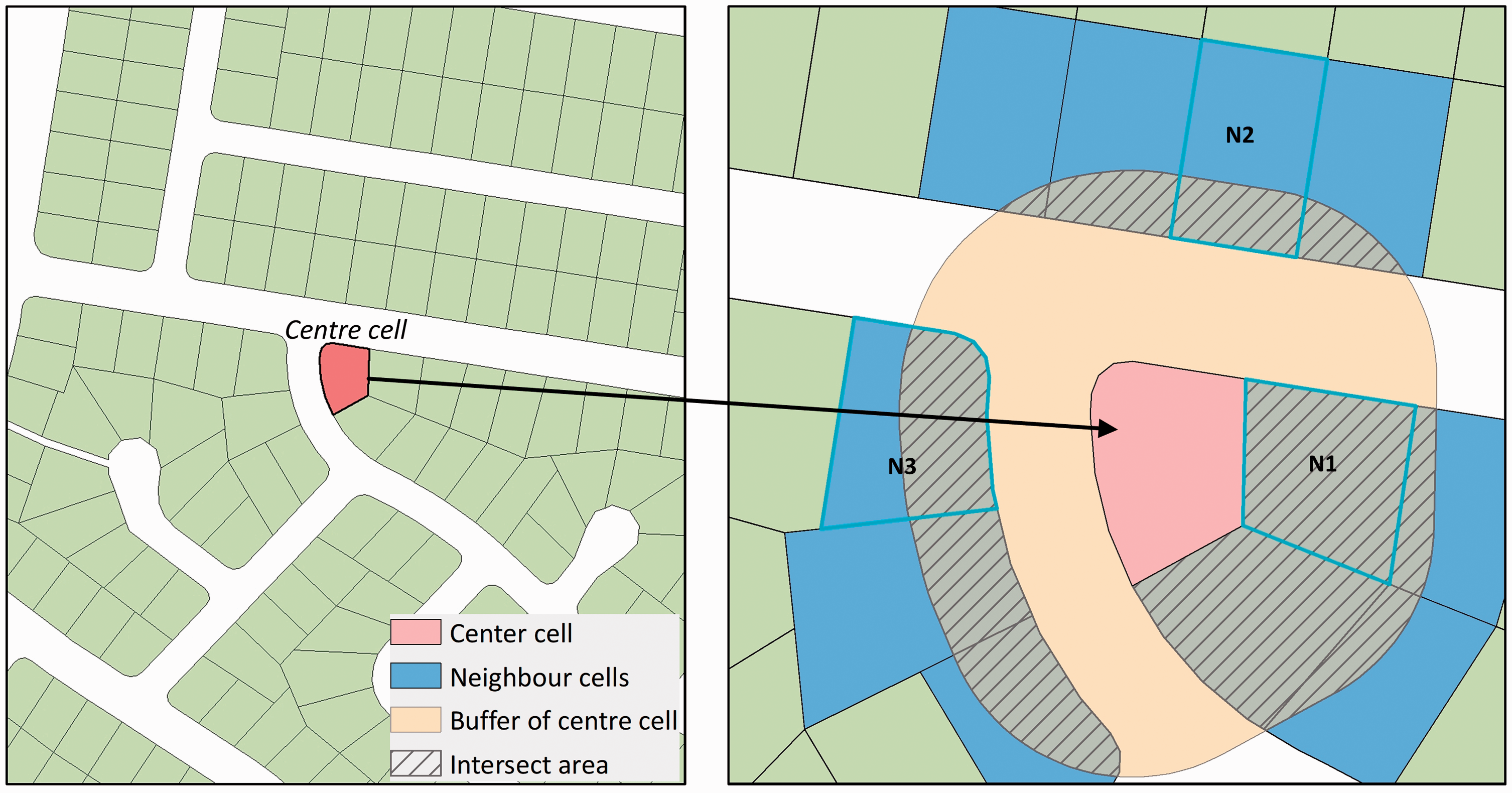
Example neighbourhood configuration of vector CA using a buffer of fixed radius.

Workflow of CA modelling

The general modelling process for raster and vector CAs are almost identical except that the vector CA includes information about the polygons (online supplementary Figure S2). Firstly, the driving factors are identified. Secondly, both vector and raster cells are extracted from the database underpinning the study area. Thirdly, the values of driving factors on cells in different formats are identified. In addition, transition rules of CA models are discovered on the basis of randomly selected sample data across the study area. Then, historical data in both vector and raster formats are imported to generate the simulated land use maps at the end of study period. Taking three spatial indicators to assess the accuracy of models is the final step.

Transition rule discovery with artificial neural networks

Transition rules are traditionally developed using multiple criteria evaluation (MCE) (Wu and Webster, 1998), principal components analysis (PCA) (Li and Yeh, 2002b), and logistic regression (Wu, 2002). Yet, they lack the ability to correct for correlations among driving factors (Li and Yeh, 2002a). With the development of artificial intelligence, more advanced methods are being introduced for the discovery and optimization of transition rules, for example ant colony optimization (ACO) (Liu et al., 2008), artificial immune system (AIS) (Liu et al., 2010), artificial neural network (ANN) (Almeida et al., 2008), bee colony optimization (BCO) (Yang et al., 2013), cuckoo search (CS) (Cao et al., 2015), differential evolution (DE) (Feng and Tong, 2018a), genetic algorithm (GA) (Liu et al., 2014), particle swarm optimization (PSO) (Feng et al., 2011), and support vector machine (SVM) (Huang et al., 2009).

In this research, ANN is applied for the definition of transition rules. An ANN consists of layers (input, hidden and output) and neurons which are analogous to the structure of human brains (Civco, 1993). The number of neurons in the input layer of ANN is equal to the number of driving factors for the CA model, so the vector ANN comprises one more neuron than the raster version since the cell shape is also considered as a factor. Significant errors have been observed in previous experiments where the size of the ANN is too small (Guan et al., 2005). Therefore, the number of neurons in the hidden layer is set as $2 j + 2$ by taking Kolmogorov’s theorem as the reference (Almeida et al., 2008; Wang, 1994), where j is the count of neurons in the input layer.

Accuracy assessment

Three indicators are used to evaluate the simulation performances of the CA models. The first one is the producer’s spatial accuracy (equation (1)), which is the proportion of correctly predicted transformed cells, using the land use map for the later time steps as the reference data.

Produce r' s spatial accuracy = \frac{C}{TC}

(1)

where

C

is the number of correctly predicted transformed cells in the raster CA model, and

TC

is the total number of transformed cells. For the vector CA,

C

and

TC

are the correct and total area of transformed cells. Besides, for any research such as this, it is important to run multiple realisations of a model to assess stability. Therefore, cumulative producer’s spatial accuracy (PA) is adopted, which refers to the average of sum accuracies in the output of vector and raster CAs (equation (2)).

Cumulative PA = \frac{\sum_{i = 1}^{n} P roduce r' s spatial accurac y_{i}}{n}

(2)

where n is the total number of simulation experiments.

The kappa coefficient (Cohen, 1960), measures inter-rater agreement for categorical items.

Kappa coefficient = \frac{p_{0} - p_{e}}{1 - p_{e}}

(3)

where

p_{0}

is the relative observed agreement among raters (identical to accuracy), and

p_{e}

is the hypothetical probability of chance agreement, using the observed data to calculate the probabilities of each observer randomly seeing each category (Viera and Garrett, 2005).

The quantity and distribution of misclassified cells has been calculated by the frequency of misclassification. ‘Misclassified cells’ are those that are simulated as changing from attribute A to B but remain A in reality, and the frequency of misclassification of a specific cell can be depicted as (equation (4))

Frequency of misclassification = \frac{N_{m}}{N_{T}}

(4)

where

N_{T}

is the total number of conducted simulation experiments, and

N_{m}

is the count a cell is misclassified. The frequency of misclassification, categorized into five intervals, measures the degree of simulation error in these misclassified cells.

Application

Study area and data processing

Ipswich City is the second oldest local government area in the Brisbane-South East Queensland (SEQ) region, Australia’s third largest metropolitan region. Ipswich City is located in the western growth corridor of the SEQ region, approximately 35 km west of Brisbane, the capital city of Queensland. It comprises an area of 1090 km², with a population of 200,000 (Ipswich City Council, 2017). It is projected by the South East Queensland Regional Plan (Queensland Government, 2017) that the resident population will be as much as 455,000 in 2031. Previous work by Stimson et al. (2012) predicted that there will be an increase of dwellings in Ipswich City from 2006 to 2016, along with urban renewal and urban consolidation. It is therefore important to understand the evolution of urban growth in Ipswich City for urban planners and policy makers to better understand the city’s future.

Two districts in the eastern part of Ipswich City are used as the study area: Collingwood Park and Redbank Plains (Figure 2). The changes in these districts are typical of Ipswich City over the study period. In 2016, the area of these two districts was 2571 ha. The main land uses are ‘Intensive uses’, ‘Production from natural environments’, and ‘Conservation and natural environments’, occupying 53.16%, 22.21% and 19.96% of the study area, respectively. The remainder of the study area comprises ‘production from Dryland agriculture and plantations’ and ‘Water’, accounting for 4.39% and 0.28% of the study area, respectively. Polygons of Collingwood Park and Redbank Plains were extracted from the local government area dataset of Queensland. This was obtained from QSpatial, a state-owned geospatial portal of Queensland (Queensland Government, 2016) which is also the source of the land use maps (1999 and 2016) and most other spatial data used in this research (online supplementary Table S1). Specific driving factors are extracted from ABS mesh block data, Baseline roads and tracks of Queensland, Land use mapping of Queensland (1999, 2016) and Protected areas of Queensland. By integrating Digital cadastral database (DCDB) and property address data, the main land use categories are identified (online supplementary Table S2).

Figure 2.

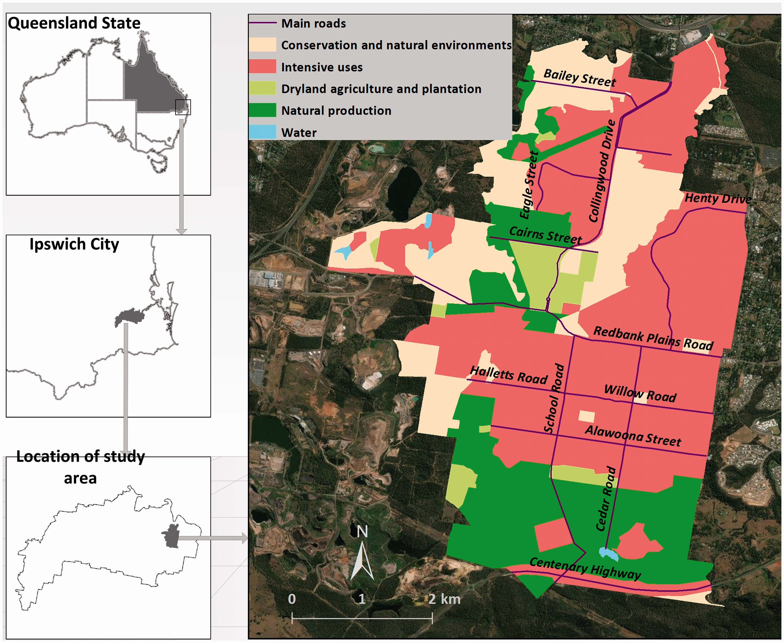
The study area is Ipswich City in Queensland, Australia. Source of satellite image: ESRI, downloaded: 06 Jan 2018.

The main land use transformation between 1999 and 2016 is from grazing native vegetation and residual native cover to residential area. The area of grazing native vegetation has been decreased by 233.95 ha between 1999 and 2016, representing 76.03% of all changed land use. Residual native cover is the category with the second largest reduction, as much as 66.3 ha, or 21.55% of the entire decreased category. There is a 200 ha increase of residential area during the same period, which is as much as 64.76% of all increased land use types.

The focus of this work is the transition of land uses to residential, thus the classification is simplified into residential and non-residential. Grazing native vegetation and residual native cover are classified as ‘non-residential’. Specifically, 188.47 ha non-residential land is being transferred into ‘residential’ during 1999 to 2016, and 809.77 ha non-residential land in year 1999 remain unchanged in 2016. These ‘non-residential’ and ‘residential’ land parcels were defined as the vector cells of our CA model. The raster cells were derived by converting the land use map into 30 m grid cells. Mesh block data, the smallest geographical area defined by Australian Bureau of Statistics (ABS, 2006, 2016), was applied to calculate population density (online supplementary Figure S3).

Driving factors

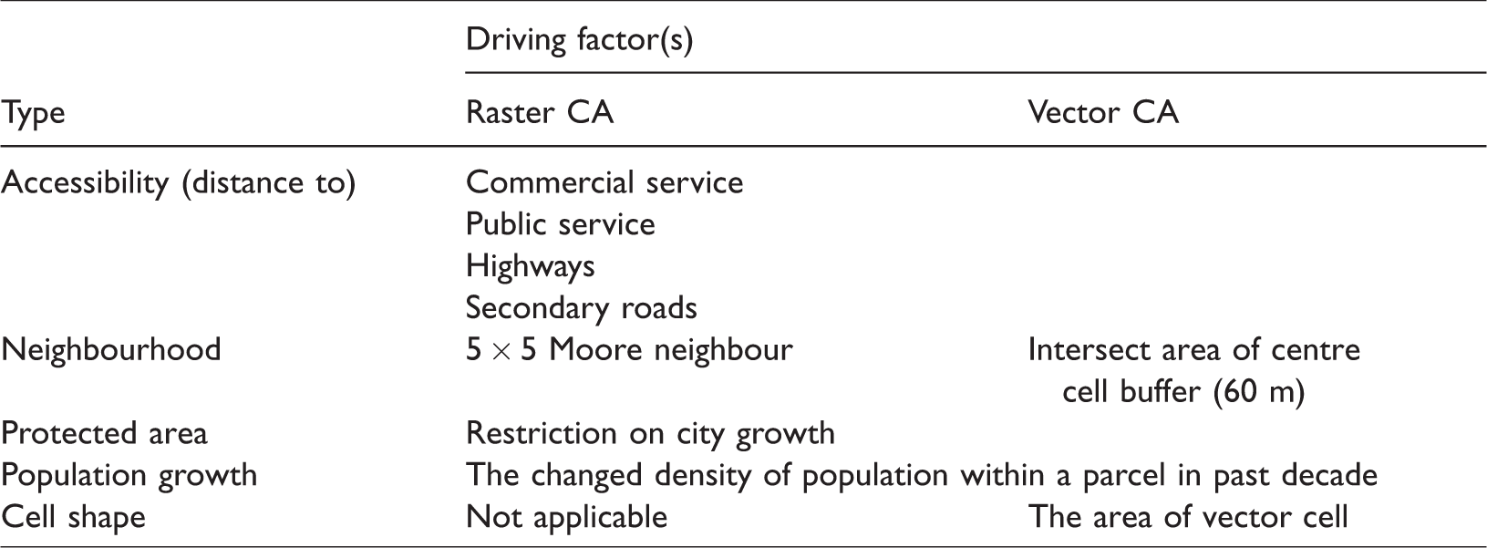
Five groups of driving factors are identified as influencing land use change for our model (Table 1): accessibility, neighbourhood, protected area, population growth and cell shape. Slope gradient is not used in this work, as 95.1% of the study area is less than 10 degrees (using 25 m DEM of the SEQ region) and its influence on land use development can be considered negligible.

Table 1.

Driving factors of land use change in the study area.

Type	Driving factor(s)
Type	Raster CA	Vector CA
Accessibility (distance to)	Commercial service
	Public service
	Highways
	Secondary roads
Neighbourhood	5 × 5 Moore neighbour	Intersect area of centre cell buffer (60 m)
Protected area	Restriction on city growth
Population growth	The changed density of population within a parcel in past decade
Cell shape	Not applicable	The area of vector cell

Accessibility

It has been confirmed by previous researchers that land use transformation is usually dependent on a series of spatial variables in terms of accessibilities or proximities (Li and Yeh, 2002a; Wang et al., 2011). Hence, distances to commercial service, public service, highways (parts of Ipswich Motorway M2 and Centenary Highway A5) and secondary roads (State Route 61), which are derived using the Near tool in ArcMap, are the four variables of the study area.

Neighbourhood configuration

A 5 × 5 Moore neighbourhood has been applied for the detection of neighbour cells in raster CA. Similarly, a buffer zone-based method has been adopted to define neighbourhood configuration of vector CA on the basis of research (Barreira-González and Barros, 2016; Moreno et al., 2009). Vector CA’s neighbourhood configuration has been identified as the intersection of the centre cell’s buffer zone and adjacent cells, which is proportional to the density of adjacent residential area. Considering the raster cell size (30 m) and radius of Moore neighbourhood (5 × 5), 60 m is set as the radius of vector neighbourhood. In raster CA, the size of each non-residential (centre) cell is 30 × 30 = 900 m², and there are 4377 residential (neighbour) cells within their neighbourhood at the beginning of simulation. For vector CA, the average size of all non-residential (centre) cells is 1711 m², excluding four cells exceeding 400,000 m² in area, and the total area of their neighbour cells is 7,697,694 m². Considering this, the ratio of neighbour cells’ area with centre cells is quite similar: 4377 for raster and 4498 for vector CAs, and therefore 60 m is a reasonable radius for vector CA.

Protected area

The spatial extent of protected areas, which represents areas reserved for the conservation of natural and cultural values, is a restriction for urban growth. Namely, no transfer is permitted within the range of protected areas.

Population growth

The difference of population densities between years 2006 and 2016, which could reflect the variation of migration, has been accepted as a key component of urbanization process by previous researchers (Han et al., 2009). Considering the linear growth trend of population in Ipswich City since the beginning of this century (idcommunity, 2016), as well as data availability, the variation of population density during past decade is the fourth group of driving factor.

Cell shape

Due to the diversity forms of vector cells, it is necessary to use their area as inputs to the calibration of vector CA model.

Model implementation

In year 1999, there were 4537 non-residential vector cells in 1999, of which 3152 (188.47 ha) were transformed into residential by 2016. The number of transformed and stable (those polygons that remain unchanged between time periods) raster cells are 2121 and 9091. For the purpose of ANN training, a random sample method has been adopted here. 50% of transformed cells and stable cells were randomly selected for training. The same number of raster cells for each model run was sampled to maintain the same ratio of area as the polygons in vector CA. The sampled data were imported to MATLAB R2014a for ANN calibration, where 70%, 15% and 15% of the sample data was used for training, validation and testing, respectively. Afterwards, the weights and biases of ANN are determined, and these are used as the transition rules of our CA models.

The number of iterations (time steps) required to ensure that spatial details can be simulated by CA models is often between 100 to 200 (Cao et al., 2015; Yeh and Li, 2006). Accordingly, the number of iteration is set to 100, with each iteration corresponding to 2 months given the simulated period (1999–2016). Each iteration comprises four steps. The first step is to calculate the values of driving factors on cells, normalizing them using the linear scaling function. The calculation of transfer probability is the next step. As equations (1) to (4) indicate, the inputs of ANN are normalized values of driving factors on cells, and the outputs of ANN is the transfer probability of each non-residential cell, which is the foundation of selection. The third step is to determine which of these non-residential cells will be transformed. When the area (vector format) or number (raster format) of selected cells reaches the pre-set threshold, which is derived from the overall change of study area during 1999–2016, the selection process is completed. In this paper, thresholds are set as 18,847 m² and 21 polygons in raster and vector CAs. The final step is to update the land use data of the study area in order to calculate the fields of driving factors for the following iteration. Once all iterations are finished, the output of the experiment is the simulated land use map in year 2016. The prototype system of CA models has been programmed using ArcObjects 10.3 software development kit (SDK) on the Visual Studio 2013 platform.

Simulation results

A series of model realisations were run to assess the variability of the model results, ending when the cumulative mean and standard deviation of the producer’s accuracy had stabilised. The ratio of sample data in each simulation experiment (both vector and raster, for each of the simulations) is listed in online supplementary Table S3. Afterwards, these sample data are applied for the training of ANN in each simulation experiment.

Figure 3 illustrates the process of land use simulation produced by the raster and vector CA models for one realisation of each model type. We used four colours to indicate the spatial distribution of cells: correctly predicted non-residential (Umber), incorrectly predicted non-residential (Blue), correctly predicted residential (Red) and incorrectly predicted residential (Purple). The newly transformed residential cells between years 1999 and 2016 reveal a rapid trend of urban expansion, particularly around the middle of the study region. At the beginning of simulation, the majority of north-western and southern parts of Redbank Plains are non-residential. Similarly, residential cells in Collingwood Park are mainly located around the middle of the regional centre, with a southwest – northeast distribution. When the CA models have completed 20 iterations of the simulation, dispersed non-residential cell which were in close proximity to residential areas in Redbank Plains, as well as those situated in the southwest of residential area in Collingwood Park, have been transformed to residential cells (Figure 3(A) and (B)). The difference between vector and raster CAs was that more newly developed residential cells, generated by raster CA, occur along the middle of Henty Drive. In vector CA, extra residential cells appeared on the south of Eagle Street in the northern part of study area. It is also indicated by the output of CA model that this trend continued when it came to the end of 60 iterations’ simulation progress with more residential cells developed in the south parts of two districts, and northeast part of Redbank Plains (Figure 3(C) and (D)). Therefore, the new residential cells in vector CA were more clustered in the southern part of the study area. At the end of the simulation experiment, a greater number of cells between Rhondda Road Reserve and residential area in Collingwood Park were transformed from non-residential to residential, which was approximately equal to half of the residential cells in year 1999. In addition, new residential cells in the northeast part of Redbank Plains were detected, which connected the two-separated residential area into a whole. Besides, additional residential cells were observed in the south direction of 1999 residential area (Figure 3(E) and (F)), mainly along Alawoona Street, Cedar Road, School Road and Halletts Road, the main roads of Redbank Plains in north-south and east-west directions. It was also demonstrated by the comparison of simulation outputs that the difference can still be detected at the edge of residential areas.

Figure 3.

Simulation process of land evolution using raster and vector CAs. Locations are labelled in Figure 2. Source of satellite image: ESRI, imagery downloaded: 18 April 2018.

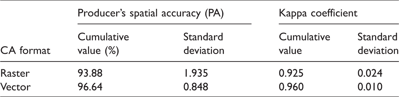
The cumulative producer’s spatial accuracies (PA) of the model realisations had stabilised by thirty realisations at 96.64% and 93.88% for the vector and raster CA models, respectively (Table 2 and Figure 4). Additionally, the average standard deviation of vector CA’s accuracy is 0.848, substantially less than for the raster CA which is 1.935. The cumulative kappa coefficient of vector and raster CA models are 0.960 and 0.925 after the 30 realisations.

Figure 4.

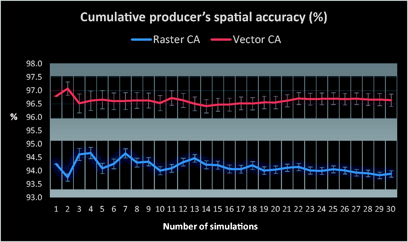
Cumulative producer’s spatial accuracy of CA models.

Table 2.

Overall error statistics.

CA format	Producer’s spatial accuracy (PA)		Kappa coefficient
CA format	Cumulative value (%)	Standard deviation	Cumulative value	Standard deviation
Raster	93.88	1.935	0.925	0.024
Vector	96.64	0.848	0.960	0.010

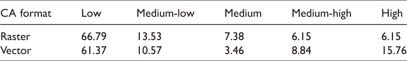
The frequency of misclassification for all misclassified cells across the 30 realisations are divided into five categories in Table 3 and Figure 5: low, medium-low, medium, medium-high, and high. These correspond to the value ranges [1, 6], [7, 12], [13, 18], [19, 24] and [25, 30], respectively. For instance, if a cell has been identified as ‘misclassified’ in 5 out of 30 simulation experiments, it will be classified as low frequency.

Figure 5.

Distribution of misclassified cells in raster (a) and vector (b) CA models. Source of base map: ESRI.

Table 3.

Frequency of misclassification (%).

CA format	Low	Medium-low	Medium	Medium-high	High
Raster	66.79	13.53	7.38	6.15	6.15
Vector	61.37	10.57	3.46	8.84	15.76

Discussion

The simulation results show that the vector CA approach has higher producer’s accuracy and kappa coefficient values than the raster CA. While the raster CA values are also high, there is no overlap between the two sets of accuracies. The cumulative producer’s spatial accuracy of the vector CA model has values ranging between 97.07 and 96.42, whereas the maximum and minimum values for the raster CA are 94.66 and 93.76. In addition, in all 30 realisations, the vector CA always has a higher cumulative producer’s spatial accuracy, and the differences between vector and raster CAs are in the range of [1.91, 3.32]. A similar situation occurs with the kappa coefficient, for which the maximum and minimum values for the vector CA are 0.98 and 0.94, and 0.96 and 0.88 for the raster CA. Therefore, the outputs of the vector CA are more accurate than the raster CA. This is in agreement with the findings of other researchers (Barreira-González et al., 2015; Moreno et al., 2009; Wang and Marceau, 2013).

There is also an obvious difference between the frequencies of misclassification in the vector and raster CAs (Table 3). For the raster CA, 66.79% of misclassified cells are misclassified with a low frequency. Furthermore, 13.53% and 7.38% of misclassified cells belong to medium-low and medium frequency of misclassification. The remainder of the misclassified cells can be categorized as medium-high and high. Regarding the misclassified cells from vector CA, low frequency of misclassification is also most common, accounting for 61.37% of all incorrectly classified cell area. Nevertheless, high frequency of misclassification ranks the second in the output of vector CA, which is 15.76%. The ratio of medium-low and medium-high misclassified cells is the third and fourth largest category (10.57% and 8.84%). Finally, the remaining 3.46% of misclassified cells have a medium frequency of misclassification.

The spatial distribution of misclassified cells provides useful information. The misclassified raster CA cells are distributed across the study region, with three obvious groups: the west edge of Collingwood Park, the east side of Collingwood Drive, and areas located to the south of Halletts Road. Furthermore, other misclassified cells are dispersed in the northwest, and east parts of Redbank Plains. Considering the misclassified cells that were generated by vector CA, their distribution is relatively concentrated, with more than 80% located in the west edge and middle of Collingwood Park, mainly around the residential area in year 1999. Generally speaking, the distribution of misclassified cells produced by the vector CA is more concentrated, which confirms that it has a better capability of error control and would be more beneficial for the work of model calibration.

It is also worth noting that the vector CA has faster processing times. For the analyses described here, the vector CA processing time was 24.3% that of the raster CA, while also resulting in a higher accuracy. This time difference is largely related to the number of spatial units in the simulations, and the average size of the polygons used in these analyses was approximately 2.5 times the raster cell size. It is worth considering how this applies to finer resolution data sets. If higher resolution satellite images are used to generate the land use maps then there would be a quadratic scaling in the number of grid cells and thus processing times, but one would not expect a substantial change in the number of land use polygons, thus the differences of processing times will diverge substantially as spatial resolutions increase.

Conclusions

In this research, the structure, parameters and workflow of vector and raster CAs have been compared, with a summarization of their similarities and differences. Collingwood Park and Redbank Plains, two districts of Ipswich City, Queensland, Australia, were used as a case study. Between 1999 and 2016, a 35.15% increase of the residential land occurred in the study area, much in a southerly direction, but also near existing residential area from 1999. We can conclude from the results of 30 realisations that the cumulative producer’s spatial accuracy of vector-based CA is 2.76% higher than raster-based CA. Additionally, the cumulative kappa coefficient of vector CA is 0.035 higher than that of the raster CA. Besides, the misclassified cells produced by vector CA have a higher spatial concentration. It is demonstrated that the vector CA model can not only produce a more accurate result in both macro and micro scales, but also narrow down the spatial distribution of misclassified outputs, which lay a solid foundation of the following work on model calibration and optimization.

The simulation and analysis results confirm that the vector-based CA model generates a more authentic output on urbanization process of the study area. Considering this, vector-based CA model could be an applicable tool to analyse the regulations and patterns of urban growth and aid the decision making of city planners. Therefore, the research of CA theories and applications on vector format is necessary and meaningful.

Supplemental Material

Supplemental Material1 - Supplemental material for Land use change simulation and analysis using a vector cellular automata (CA) model: A case study of Ipswich City, Queensland, Australia

Supplemental material, Supplemental Material1 for Land use change simulation and analysis using a vector cellular automata (CA) model: A case study of Ipswich City, Queensland, Australia by Yi Lu, Shawn Laffan, Chris Pettit and Min Cao in Environment and Planning B: Urban Analytics and City Science

Supplemental Material

Supplemental Material2 - Supplemental material for Land use change simulation and analysis using a vector cellular automata (CA) model: A case study of Ipswich City, Queensland, Australia

Supplemental material, Supplemental Material2 for Land use change simulation and analysis using a vector cellular automata (CA) model: A case study of Ipswich City, Queensland, Australia by Yi Lu, Shawn Laffan, Chris Pettit and Min Cao in Environment and Planning B: Urban Analytics and City Science

Supplemental Material

Supplemental Material3 - Supplemental material for Land use change simulation and analysis using a vector cellular automata (CA) model: A case study of Ipswich City, Queensland, Australia

Supplemental material, Supplemental Material3 for Land use change simulation and analysis using a vector cellular automata (CA) model: A case study of Ipswich City, Queensland, Australia by Yi Lu, Shawn Laffan, Chris Pettit and Min Cao in Environment and Planning B: Urban Analytics and City Science

Supplemental Material

Supplemental Material4 - Supplemental material for Land use change simulation and analysis using a vector cellular automata (CA) model: A case study of Ipswich City, Queensland, Australia

Supplemental material, Supplemental Material4 for Land use change simulation and analysis using a vector cellular automata (CA) model: A case study of Ipswich City, Queensland, Australia by Yi Lu, Shawn Laffan, Chris Pettit and Min Cao in Environment and Planning B: Urban Analytics and City Science

Supplemental Material

Supplemental Material5 - Supplemental material for Land use change simulation and analysis using a vector cellular automata (CA) model: A case study of Ipswich City, Queensland, Australia

Supplemental material, Supplemental Material5 for Land use change simulation and analysis using a vector cellular automata (CA) model: A case study of Ipswich City, Queensland, Australia by Yi Lu, Shawn Laffan, Chris Pettit and Min Cao in Environment and Planning B: Urban Analytics and City Science

Supplemental Material

Supplemental Material6 - Supplemental material for Land use change simulation and analysis using a vector cellular automata (CA) model: A case study of Ipswich City, Queensland, Australia

Supplemental material, Supplemental Material6 for Land use change simulation and analysis using a vector cellular automata (CA) model: A case study of Ipswich City, Queensland, Australia by Yi Lu, Shawn Laffan, Chris Pettit and Min Cao in Environment and Planning B: Urban Analytics and City Science

Footnotes

Acknowledgements

The authors are thankful for valuable feedback from anonymous referees and the journal editor, as well as the data provided by the Australian Bureau of Statistics (ABS) and Queensland Spatial Catalogue (QSpatial).

Declaration of conflicting interests

The author(s) declared no potential conflicts of interest with respect to the research, authorship, and/or publication of this article.

Funding

The author(s) disclosed receipt of the following financial support for the research, authorship, and/or publication of this article: The Major State Basic Research Development Program of China (no. 2015CB954101), the National Natural Science Foundation of China (grant no. 41671385), and the scholarship from China Scholarship Council (CSC).

Supplemental material

Supplemental material for this article is available online.

Yi Lu is a PhD student in University of New South Wales. His main research interest is land use change models, spatial analysis, and planning support system.

Shawn Laffan research interests are in geospatial analysis and geocomputation.

Chris Pettit is the inaugural Chair of Urban Science at the University of New South Wales. His expertise is in the convergence of the fields of Urban Planning and Geographical Information Sciences (GIS). His recent interests also span into applications, development and the critique of geographical visualisation tools including, advanced spatial decision support systems and city dashboards.

Min Cao research interests are in geographic modelling and spatial data mining.

References

ABS (2006) 2006 Census: Mesh Blocks. Available at: www.abs.gov.au/ausstats/abs@.nsf/mf/1209.0.55.002/ (accessed 1 February 2019).

ABS (2016) 2016 Census: Mesh Blocks. Available at: www.abs.gov.au/ausstats/abs@.nsf/mf/1270.0.55.001 (accessed 1 February 2019).

Almeida

Gleriani

Castejon

, et al. (2008) Using neural networks and cellular automata for modelling intra-urban land-use dynamics. International Journal of Geographical Information Science 22: 943–963.

Barreira-González

Barros

(2017) Configuring the neighbourhood effect in irregular cellular automata based models. International Journal of Geographical Information Science 31: 617–636.

Barreira-González

Aguilera-Benavente

Gómez-Delgado

(2019) Implementation and calibration of a new irregular cellular automata-based model for local urban growth simulation: The MUGICA model. Environment and Planning B: Urban Analytics and City Science 46: 243--263.

Barreira-González

Gómez-Delgado

Aguilera-Benavente

(2015) From raster to vector cellular automata models: A new approach to simulate urban growth with the help of graph theory. Computers, Environment and Urban Systems 54: 119–131.

Batty

(2009) Urban modeling. In Thrift

Kitchin

(eds) International Encyclopedia of Human Geography. Oxford: Elsevier.

Batty

Xie

(1994) From cells to cities. Environment and Planning B: Planning and Design 21: S31–S48.

Cao

Tang

Shen

, et al. (2015) A new discovery of transition rules for cellular automata by using cuckoo search algorithm. International Journal of Geographical Information Science 29: 806–824.

10.

Civco

(1993) Artificial neural networks for land-cover classification and mapping. International Journal of Geographical Information Science 7: 173–186.

11.

Clarke

Hoppen

Gaydos

(1997) A self-modifying cellular automaton model of historical urbanization in the San Francisco Bay area. Environment and Planning B: Planning and Design 24: 247–261.

12.

Cohen

(1960) A coefficient of agreement for nominal scales. Educational and Psychological Measurement 20: 37–46.

13.

Couclelis

(1989) Macrostructure and microbehavior in a metropolitan area. Environment and Planning B: Planning and Design 16: 141–154.

14.

Feng

Tong

(2018a) Calibration of cellular automata models using differential evolution to simulate present and future land use. Transactions in GIS 22: 582–601.

15.

Feng

Tong

(2018b) Dynamic land use change simulation using cellular automata with spatially nonstationary transition rules. GIScience & Remote Sensing 55: 678–2.

16.

Feng

Liu

Tong

, et al. (2011) Modeling dynamic urban growth using cellular automata and particle swarm optimization rules. Landscape and Urban Planning 102: 188–196.

17.

Flache

Hegselmann

(2001) Do irregular grids make a difference? Relaxing the spatial regularity assumption in cellular models of social dynamics. Journal of Artificial Societies and Social Simulation 4: 6.1--6.27.

18.

Geertman

Toppen

Stillwell

(2013) Planning Support Systems for Sustainable Urban Development. London: Springer.

19.

Guan

Wang

Clarke

(2005) An artificial-neural-network-based, constrained CA model for simulating urban growth. Cartography and Geographic Information Science 32: 369–380.

20.

Han

Hayashi

Cao

, et al. (2009) Application of an integrated system dynamics and cellular automata model for urban growth assessment: A case study of Shanghai, China. Landscape and Urban Planning 91: 133–141.

21.

Huang

Xie

Tay

, et al. (2009) Land-use-change modeling using unbalanced support-vector machines. Environment and Planning B: Planning and Design 36: 398–416.

22.

idcommunity (2016) City of Ipswich, population and dwellings. Available at: https://profile.id.com.au/ipswich/population (accessed 1 February 2019).

23.

Ipswich City Council (2017) About Ipswich. Available at: www.ipswich.qld.gov.au/about_ipswich (accessed 1 February 2019).

24.

Jantz

Goetz

Shelley

(2004) Using the SLEUTH urban growth model to simulate the impacts of future policy scenarios on urban land use in the Baltimore-Washington metropolitan area. Environment and Planning B: Planning and Design 31: 251–271.

25.

Klosterman

Pettit

(2005) An update on planning support systems. Environment and Planning B: Planning and Design 32: 477–484.

26.

Liu

(2008) Embedding sustainable development strategies in agent‐based models for use as a planning tool. International Journal of Geographical Information Science 22: 21–45.

27.

Yeh

AG-O

(2002a) Neural-network-based cellular automata for simulating multiple land use changes using GIS. International Journal of Geographical Information Science 16: 323–343.

28.

Yeh

AG-O

(2002b) Urban simulation using principal components analysis and cellular automata for land-use planning. Photogrammetric Engineering and Remote Sensing 68: 341–351.

29.

Liu

(2010) Intelligent GIS and Spatial Optimization. Beijing: Science Press.

30.

Yeh

AG-O

Liu

, et al. (2007) Geographical Simulation Systems: Cellular Automata and Multi-Agents. Beijing: Science Press.

31.

Liang

Liu

, et al. (2018) Delineating multi-scenario urban growth boundaries with a CA-based FLUS model and morphological method. Landscape and Urban Planning 177: 47–63.

32.

Liu

(2008) Modelling Urban Development with Geographical Information Systems and Cellular Automata. Boca Raton: CRC Press.

33.

Liu

, et al. (2008) A bottom‐up approach to discover transition rules of cellular automata using ant intelligence. International Journal of Geographical Information Science 22: 1247–1269.

34.

Liu

Shi

, et al. (2010) Simulating land-use dynamics under planning policies by integrating artificial immune systems with cellular automata. International Journal of Geographical Information Science 24: 783–802.

35.

Liu

Liang

, et al. (2017) A future land use simulation model (FLUS) for simulating multiple land use scenarios by coupling human and natural effects. Landscape and Urban Planning 168: 94–116.

36.

Liu

Feng

Pontius

(2014) Spatially-explicit simulation of urban growth through self-adaptive genetic algorithm and cellular automata modelling. Land 3: 719–738.

37.

Long

(2017) Simulating block-level urban expansion for national wide cities. Sustainability 9: 879.

38.

Long

Zhang

(2015) Land-use pattern scenario analysis using planner agents. Environment and Planning B: Planning and Design 42: 615–637.

39.

Cao

Zhang

(2015) A vector-based Cellular Automata model for simulating urban land use change. Chinese Geographical Science 25: 74–84.

40.

Mahiny

Clarke

(2012) Guiding SLEUTH land-use/land-cover change modeling using multicriteria evaluation: Towards dynamic sustainable land-use planning. Environment and Planning B: Planning and Design 39: 925–944.

41.

Ménard

Marceau

(2005) Exploration of spatial scale sensitivity in geographic cellular automata. Environment and Planning B: Planning and Design 32: 693–714.

42.

Moreno

Wang

Marceau

(2009) Implementation of a dynamic neighborhood in a land-use vector-based cellular automata model. Computers, Environment and Urban Systems 33: 44–54.

43.

O‘Sullivan

(2001) Graph-cellular automata: A generalised discrete urban and regional model. Environment and Planning B: Planning and Design 28: 687–705.

44.

Pettit

(2005) Use of a collaborative GIS-based planning-support system to assist in formulating a sustainable-development scenario for Hervey Bay, Australia. Environment and Planning B: Planning and Design 32: 523–545.

45.

Pettit

Klosterman

Delaney

, et al. (2015) The online What if? Planning Support System: A land suitability application in Western Australia. Applied Spatial Analysis and Policy 8: 93–112.

46.

Queensland Government (2016) Queensland Spatial Catalogue (QSpatial). Available at: http://qldspatial.information.qld.gov.au/catalogue/custom/index.page (accessed 1 February 2019).

47.

Queensland Government (2017) South East Queensland Regional Plan 2009–2031. Available at: www.ipswich.qld.gov.au/__data/assets/pdf_file/0005/7916/seq-regional-plan-2009.pdf (accessed 1 February 2019).

48.

Shahumyan

Moeckel

(2017) Integration of land use, land cover, transportation, and environmental impact models: Expanding scenario analysis with multiple modules. Environment and Planning B: Urban Analytics and City Science 44: 531–552.

49.

Stimson

Bell

Corcoran

, et al. (2012) Using a large scale urban model to test planning scenarios in the Brisbane‐South East Queensland region. Regional Science Policy & Practice 4: 373–392.

50.

Verburg

Veldkamp

(2001) The role of spatially explicit models in land-use change research: A case study for cropping patterns in China. Agriculture, Ecosystems & Environment 85: 177–190.

51.

Verburg

de Nijs

van Eck

, et al. (2004a) A method to analyse neighbourhood characteristics of land use patterns. Computers, Environment and Urban Systems 28: 667–690.

52.

Verburg

Schot

Dijst

, et al. (2004b) Land use change modelling: Current practice and research priorities. GeoJournal 61: 309–324.

53.

Viera

Garrett

(2005) Understanding interobserver agreement: The kappa statistic. Family Medicine 37: 360–363.

54.

Wang

(1994) The use of artificial neural networks in a geographical information system for agricultural land-suitability assessment. Environment and Planning A 26: 265–284.

55.

Wang

Marceau

(2013) A patch‐based cellular automaton for simulating land‐use changes at fine spatial resolution. Transactions in GIS 17: 828–846.

56.

Wang

Hasbani

J-G

Wang

, et al. (2011) Identifying dominant factors for the calibration of a land-use cellular automata model using Rough Set Theory. Computers, Environment and Urban Systems 35: 116–125.

57.

White

Engelen

Uljee

(1997) The use of constrained cellular automata for high-resolution modelling of urban land-use dynamics. Environment and Planning B: Planning and Design 24: 323–343.

58.

(2002) Calibration of stochastic cellular automata: The application to rural-urban land conversions. International Journal of Geographical Information Science 16: 795–818.

59.

Webster

(1998) Simulation of land development through the integration of cellular automata and multicriteria evaluation. Environment and Planning B: Planning and Design 25: 103–126.

60.

Yang

Liu

, et al. (2018) Simulating intraurban land use dynamics under multiple scenarios based on fuzzy cellular automata: A case study of Jinzhou District, Dalian. Complexity 2018; 17.

61.

Yang

Chen

, et al. (2016) A local land use competition cellular automata model and its application. ISPRS International Journal of Geo-Information 5: 106.

62.

Yang

Tang Ga Cao

, et al. (2013) An intelligent method to discover transition rules for cellular automata using bee colony optimisation. International Journal of Geographical Information Science 27: 1849–1864.

63.

Yao

Liu

, et al. (2017) Simulating urban land-use changes at a large scale by integrating dynamic land parcel subdivision and vector-based cellular automata. International Journal of Geographical Information Science 31: 2452–2.

64.

Yeh

AG-O

(2006) Errors and uncertainties in urban cellular automata. Computers, Environment and Urban Systems 30: 10–28.

Supplementary Material

Please find the following supplemental material available below.

For Open Access articles published under a Creative Commons License, all supplemental material carries the same license as the article it is associated with.

For non-Open Access articles published, all supplemental material carries a non-exclusive license, and permission requests for re-use of supplemental material or any part of supplemental material shall be sent directly to the copyright owner as specified in the copyright notice associated with the article.

0.00 MB

0.43 MB

0.38 MB

1.85 MB

0.08 MB

0.01 MB

0.06 MB