Household-level dynamics in residential location choice modelling with a latent auction method

Abstract

A longstanding deficiency in the modelling of residential location choices is the common assumption of a single household decision-maker. This paper contributes to a growing literature on methods to capture intra-household dynamics in this decision process. A latent auction approach is employed to estimate a residential location choice model for the Greater Toronto Area. The present work extends the consideration of individual utility factors beyond simple commute time, to include frequency of automobile use, transit use, and the cost of parking at the destination. Results suggest a weakening differential between male and female roles in the residential location choice, as multi-worker households are increasing in response to increasing costs of living. The strength of the latent auction model is confirmed as a means of linking bid-rent with observed market prices. Several conclusions are drawn out of the model results, including a pattern of larger households preferring the larger and cheaper houses characteristic of suburban areas of the Greater Toronto Area.

Keywords

Residential location choice bid auction intra-household dynamics discrete choice models

Introduction

Dual-worker households are an increasingly important subset of household arrangements in the analysis of transportation behaviour. Increasing costs of living relative to wages necessitate additional sources of income for the household. The proportion of dual-worker households in Canada rose from 38% in 1976 to 70% in 2015 (Statistics Canada, 2017). In the context of transportation behaviour, dual-worker households negotiate over limited resources (e.g. the number of household vehicles or mobility tools) to minimise their journey-to-work travel expenditure (time and costs). Capturing such interactions of household members and their inclination towards compromise or shared travel is critical to the modelling of residential location choices by dual-worker households. Conventional univariate decision theories are insufficient to model such choice contexts. Ho and Mulley (2015a, 2015b), as well as Akbari and Habib (2015), suggest that short- and long-term decisions (e.g. home location, auto ownership, and proximity to rail transit choices) that are conventionally modelled at the level of the household are in fact composite decisions resulting from trade-offs between members (joint decisions) of the household to achieve a reasonable level of household utility. However, applications of household level composite utility-based decision theory in transport modelling have been scarce and it is a pressing issue in household-based travel demand investigation (Picard et al., 2013). The present research contributes to this critical research gap by presenting a random utility maximisation (RUM) based joint decision model of home location choice, considering multiple worker households. Residential location choice is considered from the perspective of bid-rent, an approach which assumes locations choose the household offering the highest bid, using the latent auction approach recently proposed by Hurtubia and Bierlaire (2014). The paper exploits the latent auction approach to accommodate the intra-household interactions in home location choice modelling. This approach has been shown in Hurtubia et al. (2017) to improve upon existing methods of location and price determination used in land use forecast models. For empirical application, we use a set of revealed preference (RP) data collected in the Greater Toronto Area (GTA) and real estate statistics to estimate a model with household and individual-specific components of utility.

Literature review

The subject of intra-household dynamics came to prominence in the literature in the 1970s with seminal works by Becker (1973) and (1974). Residential location choice of multiple worker households is extensively examined in the literature (Surprenant-Legault et al., 2013), but applications in discrete choice modelling are less common.

Sermons and Koppelman (2001) develop a multinomial logit (MNL) model for two-worker households, which differentiates commute times by gender and the characteristics of the household and individuals. They consider whether each worker has a professional or non-professional job and the presence of children in the household. An intriguing component of their analysis is the inclusion of the order of residence and work relocations. They find that the order of residential change and the last work location change for the female worker is a significant factor in the residential location decision. Their utility formulation includes all variables as unweighted and they compare the importance of the male and female travel time variables based on t-tests on the paired parameter estimates (i.e. commute time parameters for each worker).

Abraham and Hunt (1997) develop a nested logit model, which simultaneously considers residential and work location choice within a nesting structure. They parameterise the scaling parameter to vary with the age and gender of the household member. However, extending this framework to consider more than two members may pose challenges in estimation due to the resulting deeply nested model structure.

At a similar time to Abraham and Hunt, Freedman and Kern (1997) derived the home location choice of two-worker households from the indirect utility function, subject to budget and time constraints. We note a few shortcomings in this early work, which has continued in much of the subsequent research. First, they begin with a budget constraint defined by the wage of both workers, cost of housing, and a composite good available to the household. However, the composite good is subsequently omitted from the model and potential wages are framed against dwelling price and commute time only. Second, the model has an a priori assumption that the husband works and the decision by the wife to work is a function of greater household responsibilities. This seems an outmoded assumption and we advocate an unbiased a priori assumption regarding the weighting of household roles on residential location choice. Chiappori et al. (2014) and Picard et al. (2013, 2015) have performed a number of studies in the area of two-worker home location choice, which build upon the microeconomic foundation of Freedman and Kern. These papers are attractive as they employ a group decision-making theory, unlike many other examples in the literature which almost exclusively utilise a unitary, or even individual, focused decision-making structure. Their models focus on the value-of-time for male and female household workers. They do not consider the effects of neighbourhood attributes or socio-demographic spatial correlations (Chiappori et al., 2014; Picard et al., 2013). This group provides a detailed review, which bridges the gap between location choice models of multiple member households and bargaining models of multiple decision-maker households. They find that the existing literature has focused on couple residential location, conditional on the workplace of each spouse. This remains a fairly traditional definition of the household, which may contain multiple workers and decision-makers who are not actively involved in the job market (i.e. stay-at-home parents, grandparents, and students). Most of the literature in family economics rely on explicit details about the intra-household bargaining process, which are difficult to obtain and even harder to operationalise for use in forecasting and prediction. In recent studies, Gupta et al. (2015) and Sanit et al. (2013) develop location choice models, with Gupta et al. introducing an interaction term to consider dynamics between the two household workers in a work location choice model.

It seems intuitive to suggest that dual-worker households travel more than one-worker households due to increased journey-to-work travel. The policy implication of this would be increased total travel with rising rates of dual-worker households. However, there is no consensus as to whether observation bears out this intuition. Much of the literature suggests that dual-worker households commute the same, if not less distance, relative to one-worker households. This issue boils down to whether partner commute distances are complements or substitutes. That is, whether households engage in intra-household trade-offs of commute distance. In a study of travel survey data in Montreal, QC, Surprenant-Legault et al. (2013) find that commute distances are complementary in that, as the distance travelled by one worker increases by 1%, so too does the distance of the other worker. However, they find the elasticity is less than one, suggesting that trade-offs in residential location choice occur such that total household commute distance increases by less than 1%. Their analysis is based on a linear regression of commute distance, with interaction considered through a variable representing partner commute distance. Regression methods provide a basis for analysis of the revealed data but do not describe the choice process. The structure of our home location choice model lends itself to modelling these conditions via its implicit representation of intra-household dynamics. The Montreal study provided that, in a traditional husband–wife household with both working, it has been found that wives typically have shorter commutes and therefore carry a stronger weight in the joint residential location choice. We can consider not only the commute distance of each household member, but also its role in determining the location choice.

Past studies of multi-worker household residential decision-making have tended to use a MNL location choice framework, as devised by Lerman (1976). In our work, we adopt a bid-rent formulation, which Martinez (1992) has proven gives equivalent results to MNL location choice under equilibrium conditions. In bid-rent (or bid-auction), it is assumed that locations are the decision-making agents and choose the household with the highest willingness-to-pay (WTP) (Ellickson, 1981). The model began as an alternative approach to hedonic price models for estimating the WTP for features of residential locations. Hurtubia and Bierlaire (2014) note the price endogeneity issue associated with the location choice approach, whereby prices are correlated with unobserved attributes of the dwelling. The bid-rent approach does not include price in the utility function and therefore does not suffer from this issue (Martinez, 1992). A measure of price is provided through the expected maximum utility (also known as logsum) of the bids across all households engaged in each location auction. This result can be adjusted to account for the monetised market price by using a variety of methods, such as that originally used by Lerman and Kern (1983).

We note that one method that is employed to consider intra-household dynamics in the literature is the multi-linear specication developed by Keeney and Kirkwood (1975). This method is most often applied in the context of allocating work, leisure, and other time among household members, but has been applied to residential location choice. One such application is by Zhang and Fujiwara (2009), who consider household preferences for transit-oriented development: housing located and designed to minimise walking distance to transit. Unfortunately, this theory was developed for cardinal utilities, whereas the RUM discrete choice models typically employed in residential location choice modelling are based on ordinal utilities. Given that utilities can be negative, it is not possible to accurately interpret the interaction terms in the multi-linear model specification. Additional details on this issue are presented in an article by Weiss and Habib (2018).

To date, there have been no applications of bid-rent theory to multi-worker home location choice. Its appeal arises from the interpretation of the choice set, which is inverted from the location choice perspective. By considering households as the choice alternatives, differences in household structure (i.e. number of workers and/or children) become characteristics of the alternatives. Taking a bid-rent approach provides a simple method for determining the price of each location as the outcome of an auction. Intra-household dynamics enter through the knowledge that household members will not have the same utility maximising perception of each location. Individual-level factors will influence the WTP for each location, such that it can be said that there is an internal sub-auction to determine the location providing the maximum aggregate bid for the household.

Model framework

The latent auction structure, with intra-household interactions, is illustrated in Figure 1 and details of its derivation follow. The discrete choice model is structured such that each observation in the dataset contains a single location and multiple households. In essence, bid-rent assumes a single location is considered by multiple households who bid on the location based on its attributes and their WTP (i.e. income and household characteristics). The location is rented to the household that is willing to pay the most for it. In location choice, we always assume that dwellings are rented rather than owned, with owned dwellings being rented by the owner to themselves.

Figure 1.

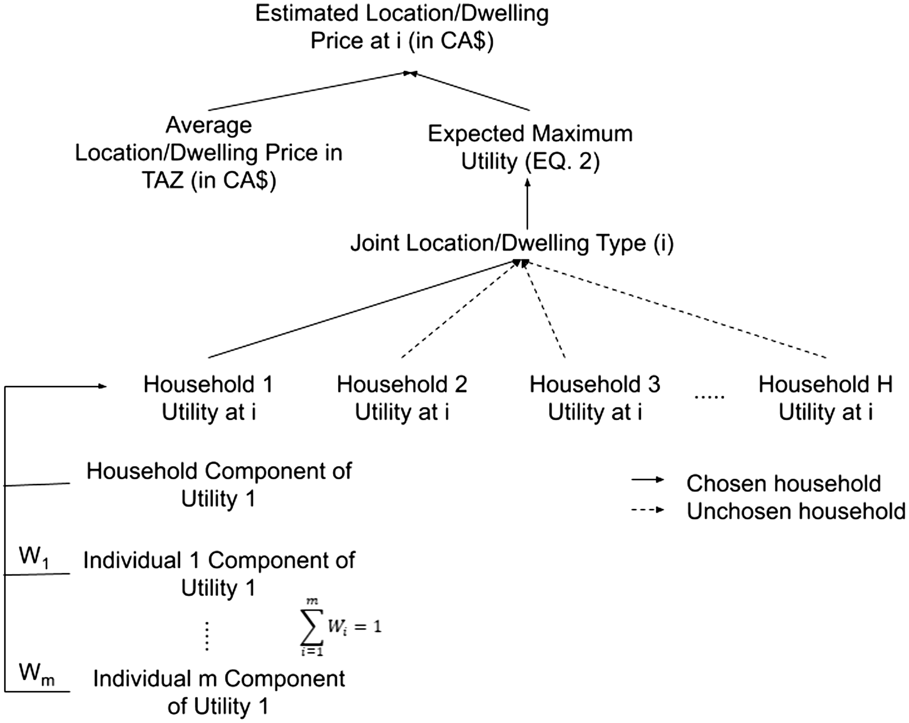
Latent auction model structure with intra-household dynamics. TAZ: traffic analysis zone.

The behavioural meaning of the bidding process can be exemplified as follows: there is a single-family dwelling in a low-density residential neighbourhood. It has three bedrooms and is located near an elementary school. We randomly select households from a survey sample who will bid on this home. The household that chose the home in reality is included in the auction and might be a family with two school-age children. They will be willing to pay for the bedrooms and proximity to schools. Another household might be randomly included in the auction that consists of a single person. They place no value on being close to an elementary school and are not willing to pay as much for additional bedrooms. They value proximity to their workplace and local bars. One could select households that are similar to the chosen household, through a choice set generation model, but this increases the complexity of the model and can lead to sample selection bias.

In developing the model, we employ the microsimulation bid-auction approach developed by Hurtubia and Bierlaire (2014), which builds upon the bid-choice theory of Martinez (1992). Model derivation begins with a standard bid-rent function (Ellickson, 1981)

P (h | i) = \frac{\exp (μ B_{hi})}{\sum_{g \in H} \exp (μ B_{gi})}

(1)

where

P (h | i)

is the probability of household h being located in traffic analysis zone (TAZ) i and μ is a scale parameter (normalised to 1.0). The bid B_hi can be parameterised as a function of zonal and household characteristics, and the winning bid expressed as a stochastic expectation

r_{i} = E (\max_{H} (B_{hi})) = \frac{1}{μ} l n (\sum_{g \in H} \exp (μ B_{gi})) + C

(2)

which, according to bid-choice theory, gives an equivalent distribution of households to the location choice formulation. The logsum term gives a standard measure of the expected maximum bid for a particular location i and where constant term C is an unknown representing the inability of the modeller to measure the absolute bid price.

The latent auction model can be applied to develop a microsimulation of the bid-choice process. The expected maximum bid can be considered a latent variable in a price model, wherein the bids of all households for a particular location are included in the price, but only in relative terms. The difference between the observed price R_i and latent auction price r_i is assumed to follow a normal distribution

f (R_{i} | r_{i}) = \frac{\exp (- \frac{R_{i} - δ - γ r_{i}}{2 σ^{2}})}{\sqrt{2 π σ^{2}}}

(3)

where δ, γ, and σ are estimated parameters representing the relationship between the observed and latent price for location i. In the present work, ‘location i’ is a composite location composed of a TAZ and a dwelling type choice (between single-family detached, townhouse, and apartment). Separate zonal prices are included in the model for each dwelling type. Assuming a mean of zero, the above function represents the probability of the observed price, given the latent price derived from the logsum auction price. The likelihood term is then a joint function of the product of the bid-rent probability and the price density function

L = P (h | i) f (R_{i} | r_{i})

(4)

We see this is an appealing framework for the development of a residential location choice model. It is consistent with the microeconomic foundations of bid-choice and provides a method for the inclusion of endogenous prices in an agent-based microsimulation model. The inclusion of intra-household dynamics is accomplished through a modification of the parameterised bid function B_hi. The decision of a residential location is a function of both household and individual-specific attributes, which can be considered through a weighted utility function. The bid function is then given by

B_{hi} = \sum_{j} β_{j} X_{hj} + \sum_{k} β_{k} Z_{hik} + \sum_{p \in h} (w_{p} \sum_{m} β_{m} X_{hm} + \sum_{n} β_{n} Z_{hin})

(5)

where X_hj are household-specific explanatory variables, Z_hik are terms that interact household and location-specific explanatory variables, X_hm are individual-specific explanatory variables, and Z_hin are terms that interact individual- and location-specific explanatory variables. The bid function is derived from the household utility where household-specific explanatory variables are common for all household members. The weights in equation (5) are applied only to individual-specific explanatory variables. Individual-specific explanatory variables differ in their values between individuals within a household. The individual weights sum to 1.0 so that the individual-specific components of the household bid function are applied with the same weight as household-specific explanatory variables. As an example, take a two-person male/female household wherein both individuals work. Each worker has a commute time, which appears in the household utility function. However, it may be the case that the household is willing to pay more to reduce the commute time of the female member. This would be associated with an unequal weight (>0.50) for the disutility associated with living further from the female place-of-work. The individual-specific weights can be parameterised as logit functions of socio-demographic characteristics as follows

w_{p} = \frac{\exp (\sum_{s} α_{s} y_{ps})}{\sum_{p \in h} \exp (\sum_{s} α_{s} y_{ps})}

(6)

where y_ps are individual-specific socio-demographic variables describing the weight of the utility associated with individual p of household h.

Description of data and study area

The empirical application is based on a survey conducted in 2014 by residents of the GTA. The survey, denoted CHOICE for Car and Household Ownership in the face of Increasing Commuting Expenses, focuses on car and home ownership decisions (Papaioannou and Habib, 2015). It includes a large set of RP data regarding car and home characteristics, as well as socio-demographic information on each responding household. Two stated preference experiments are included in the survey, focusing on mobility tool adoption and residential location choice, respectively. A total of 501 complete responses were acquired through a panel provided by a market research firm. From this sample, 413 household responses – including information on 757 individuals – are used in the present analysis. The CHOICE survey data are linked with additional statistics from the 2006 Transportation Tomorrow Survey (TTS¹) to calculate inter-zonal travel times and costs, which we update with data from the 2011 survey (DMG, 2014). The original survey application was to interregional commute trips. As such, the data do not include households who commute within their city of residence. This biases the average trip length of the sample but should not adversely affect the analysis of intra-household dynamics. A summary of key transportation statistics is provided by household in Table 1 for each of the five regions included in the analysis.

Table 1.

Descriptive Statistics for Key Household (HH) Transportation Variables.

Variable	Statistic	Durham	Halton	Peel	Toronto	York	Total
Transit pass (0/1)	Per cent of respondents by region	8.0	12.9	11.4	3.3	10.6	8.6
Auto + transit cost ($per month)	Mean	702	669	619	500	723	630
Household vehicles	Mean	1.9	2.2	1.9	1.4	2.1	1.8
Auto commute time (min)	Mean for adult male	21.8	50.2	32.0	28.6	48.1	31.8
	Mean for adult female	19.6	41.7	28.3	27.5	41.4	28.7
	Mean for dependent child	18.5	38.4	28.4	33.8	45.9	29.4
	Mean for other member	8.3	32.8	69.0	38.8		30.9

Additional data pertaining to land use were available from regional transportation models and previous data collection by the University of Toronto. Figure 2 shows the distribution of land uses by classification for each of the five regions. The GTA is a diverse region, with areas of high density commercial and residential development, sections of suburban development, and large areas still devoted to agriculture and natural land preserves. It is clear that parks and open space still dominate the region, but residential uses are not far behind (if not higher).

Figure 2.

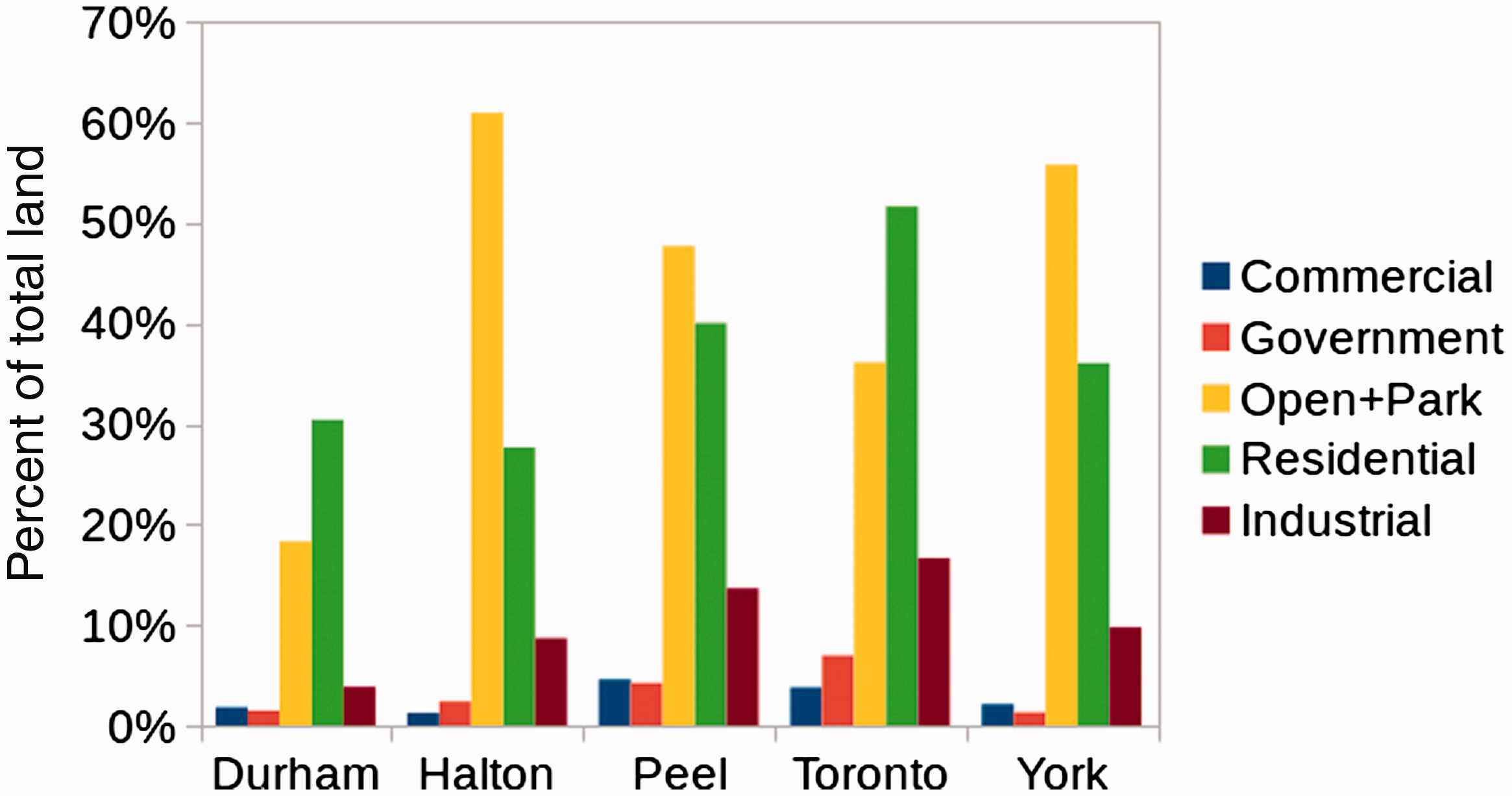
Distribution of region land uses.

The CHOICE survey includes data on home purchase price, or rent, but this does not give a clear picture of the overall market conditions and prices are given as of the year of purchase. We supplement the survey data with real estate statistics compiled by the Toronto Real Estate Board (TREB, 2017). They publish a monthly report outlining market prices aggregated to a custom set of 30 zones outside the City of Toronto and 36 zones within it. TREB classifies dwellings as detached, semi-detached, row/townhouse, condo townhouse, condo apartment, cooperative apartment, detached condo, and co-ownership apartment. We aggregate these classifications into house, townhouse, and condo for ease of analysis and to increase the sample size of each category. We further supplement these data with real estate listings (obtained from MLS) records collected in May 2017 for both owned and rented dwellings. These data also include the area of each dwelling, number of bedrooms, and number of bathrooms. Figure 3 provides annualised costs for each region and tenure type. For owned dwellings, a 25-year amortisation period is employed, with an interest rate of 5%, to obtain a representative annual cost (RBC, 2018). In the figure, each of the numbers (1,2,3) corresponds to a dwelling type (respectively, house, townhouse, and condo). It is evident that owned prices are significantly higher than rented prices; however, ownership gives the household possession of the asset and therefore includes an expected monetary return upon sale of the asset.

Figure 3.

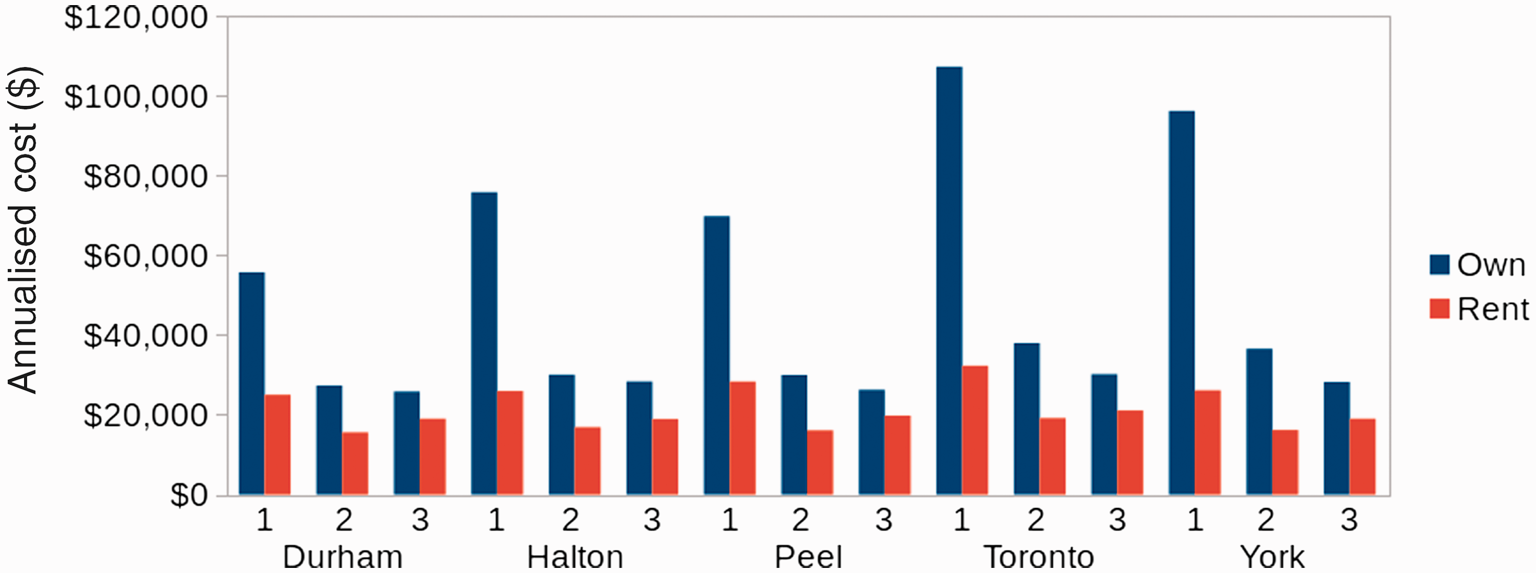
Distribution of annualised cost by region and dwelling type.

Model development

The estimation of the bid-rent model requires multiple households to bid on each TAZ-dwelling type option, with the winning household being the one that is located in that TAZ and dwelling type (e.g. a single-family dwelling in zone 1). Using the RP data collected in the CHOICE survey, we only have the chosen location of each responding household and their characteristics. McFadden (1978) has proven that consistent parameter estimation can be performed using a random sample of alternative households. Many previous studies of residential location choice use a small sample (i.e. 10 alternative households), but Nerella and Bhat (2004) provide a quantification of the error associated with smaller sampling rates. Guided by their analysis, we take the household records from the CHOICE survey and associate them with 30 randomly selected household records from among those respondents who are not located in the same TAZ, with the sample size being denoted by H. We also explored a stratified importance sampling, taking 15 records from the same region and 15 from the same income group. However, this did not improve the significance of parameters or model goodness-of-fit. We define separate zones for each of the dwelling types considered in the model (i.e. house, townhouse, and condo), representing a simultaneous choice of zone and dwelling type by each household.

In most instances, unique explanatory variables can only be derived from the interaction of zone and household-specific attributes. A summary of the variables included in the final model is provided in Table 2. For example, the commute drive time to work is a function of both the home and work location of a respondent. We assume that work locations are fixed, but the use of a record in the estimation of the expected bid in another TAZ requires an estimate of the commute time from this unchosen home location. We, therefore, link the data with an inter-zonal matrix of AM peak auto commute times from the GTA RTM. Another example of this interaction is the average dwelling area for each TAZ, which we interact with a household size of the respondent. Taking the natural logarithm of the household size provides a measure of dwelling area having a diminishing marginal influence on choice for each additional household member. In some instances, only the household attribute is used, as in the case of home to work distance. We divide this value by the income of each individual to obtain a measure of the sensitivity to commute distance as a function of additional income. We assume this sensitivity to be a characteristic of the individual, independent of the TAZ they are considering – in contrast to the commute time sensitivity, which is assumed to be fixed across respondents. The combination of these two variables accounts for the effect of proximity to the work location and differences between individuals arising from economic factors.

Table 2.

Development of model variables.

Variable	TAZ property ×	HH property
Individual variables
HW distance		Home to work commute distance/individual income
HW auto time	Inter-zonal home-to-work auto travel time (min)	Exogenous work TAZ
Park cost		Cost of parking at work location (10s $per month)
Transit	Count of GO Train stations within 3 km orTTC stations within 500 m of zone centroid	Individual has transit pass (0/1)
Frequency auto		Frequency of individual commute by auto
HW region	Home and work location in same region (0/1)	Exogenous work region
Household variables
House	House (0/1)	2+ HH members (0/1)
High income	Mean HH income in top income quintile (0/1)	HH income in top income quintile (0/1)
Low income	Mean HH income in top income quintile (0/1)	HH income in bottom income quintile (0/1)
Dwelling area	Average dwelling area (100 s m²)	ln (HH size)
Veh/lic		HH vehicles/HH licenses
Children		Number of children in HH
INC_2		HH income in second quintile
INC_3		HH income in third quintile
INC_4		HH income in fourth quintile
INC_5		HH income in top quintile
Weights
W_Role1		Adult male
W_Role2		Adult female
W_Role3		Dependent child
W_Role4		Other member
W_Age		ln (Age of HH member)

HH: Household; HW: home to work; TAZ: traffic analysis zone.

We define alternative-specific constants by the membership of each household in an income quintile. This is similar to the models developed by Hurtubia and Bierlaire (2014) in their original work. In this initial exploration of the model, we define the individual utility weights by household role. Four roles are defined as follows: adult male, adult female, dependent child, and other member. It should be noted that there is some overlap between the characteristics of individuals holding an ‘adult’ or ‘child’ role in the dataset. The ‘child’ role generally refers to individuals under the age of 18, but may include older individuals who still live with their parents (e.g. university students). This distinction is deemed valid as the weights denote the role each individual plays in determining the residential location choice. In the case of an individual, over the age of 18 and living at home, it is likely they were younger at the time of the residential location choice. In contrast, the same individual likely had a greater influence on the decision if they are listed as an ‘adult’ and they are the owner of the dwelling. This partially explains the result in Table 1. The average commute time for those given the role ‘child’ is similar to, or higher than, the ‘adult’ roles for most regions. There are two households with individuals listed as ‘child’ who are aged 35–44. With the caveat that the sample size makes this largely anecdotal, the mean commute time for these individuals is 47 minutes, which is well above the regional average.

Model results

The results of the estimation are outlined in Table 3 for the final model. A wide variety of intermediate models were estimated, including standard bid-rent models (excluding the latent auction component) for each model. The majority of the parameters are significant (at the 0.05 level of significance) and have intuitive signs. Critically, home to work auto travel time (‘HW auto travel time’) has a negative parameter and dwelling area is found to have a positive parameter, both being significant. The ‘House- 2+ members variable’ – representing the probability of a household with two, or more, members choosing a house dwelling type – has a negative sign. Looking at the corresponding bid-rent function, the sign is consistently positive in models that include this variable. Hurtubia and Bierlaire (2014) obtain a similar result for this variable, which is concentrated in more outlying areas of the GTA. These outlying areas are characterised by lower dwelling prices, relative to those in the City of Toronto proper. The negative sign on the parameter suggests that larger households, who have higher living expenses, value the lower priced houses located in the outlying suburbs. Another cause for this outcome is the large region of analysis and differences between prices not necessarily being positively correlated with the size of the dwelling, when compared between regions. Put in more specific terms, locations within the City of Toronto have a variety of amenities associated with them (e.g. better transit service, cultural facilities, variety of restaurants), which are not captured in the model. These amenities contribute towards the high prices illustrated in Figure 3, despite houses in Toronto being smaller or of a similar size to much cheaper houses in suburban regions.

Table 3.

Model parameter statistics.

Variable	Value	t-stat	Robust t-stat
Individual variables
HW auto travel time	−0.03	−12.52	−3.13
Parking cost at school or work	0.01	2.38	1.08
Transit	0.34	2.60	0.70
Frequency auto	2.08	11.46	2.51
HW region	0.55	5.25	1.33
Household variables
House - 2+ members	−0.33	−3.06	2.06
High income TAZ − High income HH	0.33	3.32	0.88
High income TAZ − Low income HH	−0.20	−0.82	−0.43
HW distance/HH income	1.09	5.39	1.21
Dwelling area	0.26	6.14	2.31
Vehicle/licenses	−0.53	−7.24	−5.52
Children	−0.16	−3.40	2.06
INC_2 (low-middle income)	0.18	0.71	0.17
INC_3 (middle income)	0.44	1.74	0.42
INC_4 (high-middle income)	0.44	1.59	0.38
INC_5 (high income)	0.47	1.79	0.42
Weights
α_Role1	0.00	0.00	0.00
α_Role2	0.08	0.44	0.16
α_Role3	−0.34	−0.62	−0.26
α_Role4	0.25	0.28	0.18
α_Age	−0.26	−0.64	−0.27
Price variables
γ	0.43	10.21	2.50
δ	9.06	44.03	9.87
σ	0.25	37.76	35.52
ρ² (const)	0.08

HH: Household; HW: home to work; TAZ: traffic analysis zone.

We find a common parameter value for locating proximate to TTC stations and GO Train stations (‘Transit’), given the bounding radii defined for each station type. This suggests that households tend to ceteris paribus value being located within 500 metres of a TTC station in a similar way to being located within 3 kilometres of a GO Train station. A negative sign is obtained for the number of vehicles per licensed driver, which suggests that households tend to trade-off a higher priced dwelling against the ownership of additional vehicles. This is consistent with other parameter values in that transit proximity is positively valued and larger households tend to locate in outlying areas, with poor transit service, requiring the purchase of additional vehicles.

With respect to individual weights, weights are estimated in the final model for four household roles (i.e. adult male, adult female, dependent child, and other). A challenge in estimating these weights is the requirement for a reference weight in the MNL weight function, against which to measure the relative utility for other household members. Household compositions in the sample are not uniform, such that a single role cannot be fixed as the reference. For example, a household may contain two adult males or no adult males. We reference the weight of each household member against the role of the responding member. It is interesting to note that this model does not suggest a strong difference in the weight of male and female influence on residential location choice – in contrast to prior studies on the subject (Chiappori et al., 2014; Picard et al., 2013). In a household with a single male/female couple, the weights are 0.49 and 0.51, respectively.

Given the aforementioned caveats about the overlap between ‘adult’ and ‘child’ roles, we included a weighting variable for the age of the household member. Although not strongly significant, this suggests that age plays a strong role in the weight of the individual on residential location choice. We explored the inclusion of several other variables, including individual work status and income, but the sample data are incomplete for these variables and their inclusion did not have a significant effect on the model.

Another avenue of exploration was considering variation in household composition by distinguishing the adult role weights based on whether the household includes children. This would account for differences in the role of an adult by their consideration for school location and altruism for their children. However, no significant difference was found between these variables. This effect is partially considered through the inclusion of the age weight and variable in the household utility function indicating whether the household includes children (under the age of 13). A series of other weight configurations were explored for adult roles including separate weights for single and multi-worker household adults, separate weights for single and multi-member household adults, and the addition of a weight for full-time work status. We also considered models wherein the individual utilities were separated into weighted and unweighted components. None of these changes significantly improved the model fit or provided statistical insights into intra-household dynamics.

We compare the final model to a series of intermediate models according to Akaike Information Criterion (AIC) and Bayesian Information Criterion (BIC) measures in Table 4. The final model offers a significant improvement over the model with unadjusted age weights. This suggests that weight has a nonlinear effect on the individual utilities. We also consider a model with equal weights, which provides a worse fit to the data and indicates estimating the weights significantly improves the model fit. A model without the latent auction component, market price data, was also estimated. This model offers a slight improvement over the model presented in this paper. However, the final model is an improvement in that it includes dynamics (noted above) resulting from unobserved variables contained in the market price. We suggest that this poorer fit is the result of the highly aggregate price data available. More granular data would likely improve upon the AIC and BIC measures calculated for the model without the latent auction component.

Table 4.

Comparison with intermediate models.

Model	Log-likelihood	AIC	BIC
Final model	−2755.77	5559.53	5757.73
Final model (unadjusted age)	−2876.83	5801.66	5999.85
Final model (equal weights)	−2898.66	5837.33	6002.49
Final model (no latent auction)	−2721.05	5484.10	5657.52

Elasticity analysis

A robust and tangible method for examining the magnitude of parameter values is obtained from calculation of the elasticities with respect to each explanatory variable. In the case of continuous variables, this takes the form of a point elasticity, while category variables require the use of an arc elasticity measured between variable states. In the latent auction model, elasticities take the form

e_{hij} = (β_{j} (1 - P (h | i)) f (R_{i} | r_{i}) + \frac{γ β_{j} P (h | i) f (R_{i} | r_{i})}{2 π σ^{2}}) Z_{hij}

(7)

for household-specific variables and

e_{hin} = (β_{n} W_{p} (1 - P (h | i)) f (R_{i} | r_{i}) + \frac{γ β_{n} W_{p} P (h | i) f (R_{i} | r_{i})}{2 π σ^{2}}) Z_{hin}

(8)

for individual-specific variables. Variables are defined as above, and e_hij and e_hin are arc elasticities for each observation with respect to household-specific variable j and individual-specific variable n, respectively. The aggregate elasticity for the sample is calculated using the probability weighted average.

We present a combined plot for a subset of continuous variables in Figure 4 (AIVTT = Auto In-Vehicle Travel Time). It is evident that there is a large positive elasticity between the price of a dwelling in a given TAZ and the average dwelling area for that TAZ-dwelling type pair. A graphical representation helps to draw out the similarity in elasticities between the adult male/female roles with respect to their sensitivity to auto travel time and parking cost at school or work. It is also clear that the influence of dependent children on residential location choice is weaker.

Figure 4.

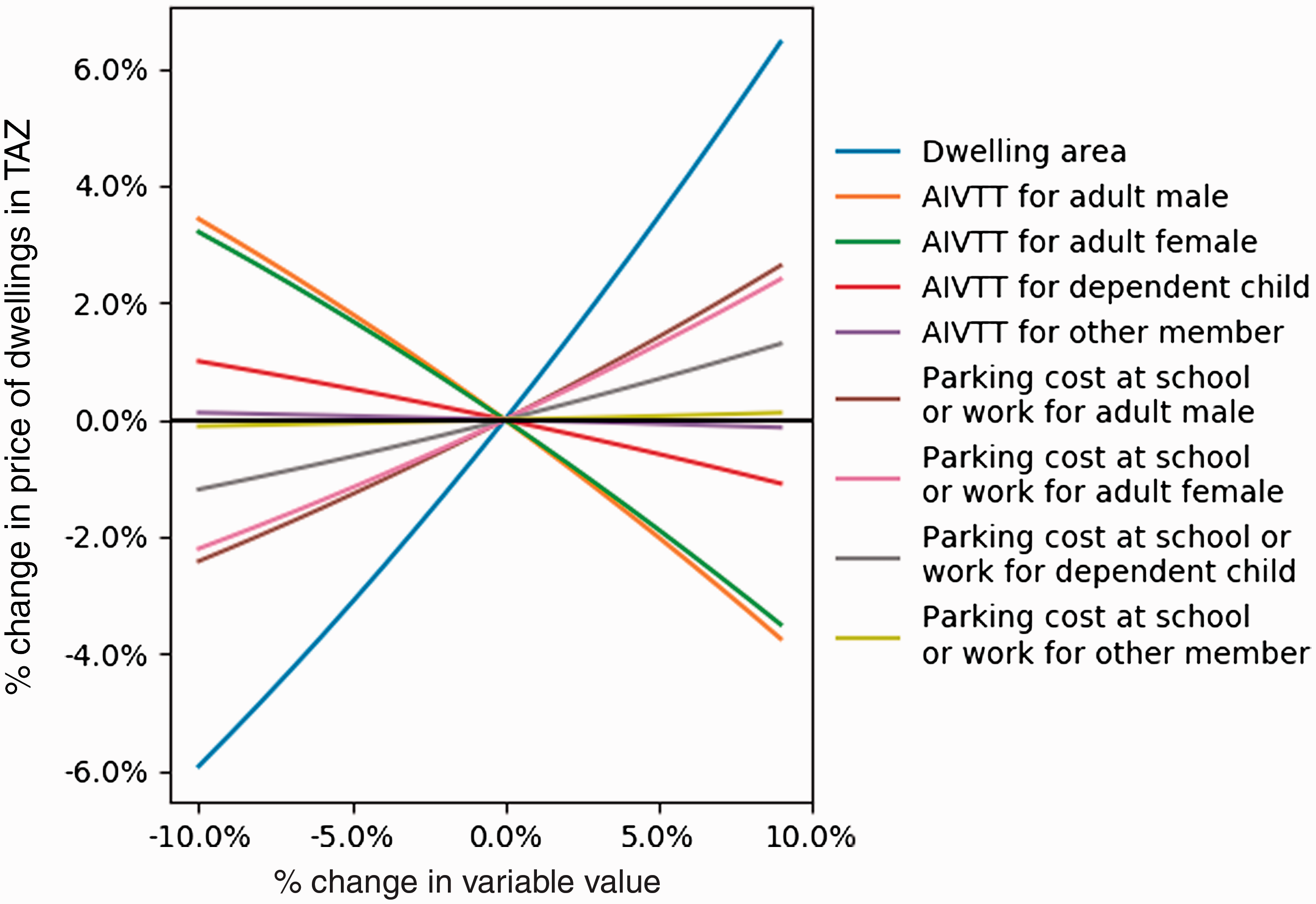
Elasticities for representative variables.

The elasticities for parking cost indicate that households are willing to pay more for a dwelling as the cost of parking rises at their work location. The elasticities do not provide direct evidence for a particular cause of this increased WTP, but there are several reasons with policy implications. A household may choose a dwelling closer to the work location to reduce the cost of travel or one close to transit to eliminate the parking cost at the work/school destination. In either case, this suggests that households are willing to pay an additional amount for a dwelling that reduces their commute costs (travel + parking). We suggest that this elasticity result provides support for parking pricing near work destinations to encourage use of transit and living closer to work – reducing the commute distance.

Conclusions and future work

This paper adds to the growing literature on intra-household dynamics in residential location choice. By considering such dynamics, we can better capture the decision-making process and consider a wider range of policy scenarios. The paper presents a latent bid-auction model considering intra-household interaction in home location choices. The present analysis suggests a weakening differential in the influence of male and female household members on residential location choice. This fits with a continued shift towards higher labour force engagement, whereby the household must consider the work location of several members. We find that larger households remain constrained in their ability to locate in urban areas, proximate to their work location. Whether this is an outcome of high land prices or a lack of available housing stock, single-family houses continue to be the domain of outlying suburban areas, with low land prices and high automobile dependence.

The methods applied in this research are found to be appealing for several reasons. The latent auction function provides a means of including market price effects, while maintaining a flexible requirement for price data. It is typical that location choice surveys do not collect price statistics, or that such statistics are given as the price at the time of purchase (i.e. not consistent in their appraisal year). The latent auction approach allowed us to use aggregate price data to provide a general pattern of prices in each area, while allowing for variation through the deviation term. The additive weighted utility is found to be a robust framework for testing various intra-household dynamics. Traditional husband/wife classifiers were not to be significant in this study, but additional exploration may elicit distinction between household roles. For example, the distribution of income between household members or cultural background of the household may affect the weighting of household roles.

This study presents a strong basis for further research. However, it could be improved through the collection of a sample that includes households who work within the same city. A major bias, existing in most residential location choice models, is the so-called modifiable areal unit problem. This arises from the use of arbitrary aggregations of spatial units, a standard practice in residential location choice models. We explored the inclusion of a spatial lag term in our model to account for this bias. Lags were considered for the co-location of similar income households, similar sized households, and by tenure (i.e. own or rent dwelling). Results are preliminary, but this direction holds promise for additional insights with respect to household dynamics and social effects. We also plan a stronger integration with the auto ownership decision for future work. There is a strong endogeneity between the travel modes available to a household and its residential location choice.

Footnotes

Acknowledgements

The authors are grateful to the attendees of IATBR and TRB for their helpful comments during earlier presentations of this research. The authors acknowledge the help of Elli Papiaoannou in initial data preparation. However, the authors are solely responsible for all discussion, interpretation, and comments.

Declaration of conflicting interests

The author(s) declared no potential conflicts of interest with respect to the research, authorship, and/or publication of this article.

Funding

The author(s) disclosed receipt of the following financial support for the research, authorship, and/or publication of this article: The study was partially funded by an NSERC Graduate Scholarship and an NSERC Discovery Fund.

Note

Jason Hawkins is a PhD candidate in Civil and Mineral Engineering at the University of Toronto.

Adam Weiss is a Postdoctoral Fellow in Civil and Environmental Engineering at the University of Calgary.

Khandker Nurul Habib is a Professor in Civil and Mineral Engineering at the University of Toronto.

References

Abraham

Hunt

(1997) Specification and estimation of nested logit model of home, workplaces, and commuter mode choices by multiple-worker households. Transportation Research Record: Journal of the Transportation Research Board 1606: 17–24.

Akbari

Habib

(2015) An econometric investigation on the relationship between modal accessiblity and the home-work spatial configuration of two-commuter households. Transportmetrica A: Transport Science 11(10): 897–917.

Becker

(1973) A theory of marriage: Part I. Journal of Political Economy 81(4): 813–846.

Becker

(1974) A theory of marriage: Part II. Journal of Political Economy 82(2): 11–26.

Chiappori

Inoa

de Palma

, et al. (2014) Couple residential location and spouses workplaces. In: III Workshop on Urban Economics, June 9–10, Barcelona: 34URL http://www.sustaincity.org/publications/WP_3.3_Couple_Chaippori_de_Palma_Picard.pdf (accessed 29 September 2017).

DMG (2014) 2011 TTS: Design and conduct of the survey. Technical report, University of Toronto. Available at: http://dmg.utoronto.ca/pdf/tts/2011/conduct2011.pdf (accessed 15 June 2018).

Ellickson

(1981) An alternative test of the hedonic theory of housing markets. Journal of Urban Economics 9(1): 56–79.

Freedman

Kern

(1997) A model of workplace and residence choice in two-worker households. Regional Science and Urban Economics 27: 241–260.

Gupta

Vovsha

Anderson

(2015) Workplace location choice with coordination between multiple workers in the household. TRB 94th Annual Meeting Compendium of Papers 3(2493): 1–22.

10.

Mulley

(2015a) Intra-household interactions in tour-based mode choice: The role of social, temporal, spatial, and resource constraints. Transport Policy 38: 52–63.

11.

Mulley

(2015b) Intra-household interactions in transport research: A review. Transport Reviews 35(1): 33–55.

12.

Hurtubia

Bierlaire

(2014) Estimation of bid functions for location choice and price modeling with a latent variable approach. Networks and Spatial Economics 14: 47–65.

13.

Hurtubia

Martinez

Bierlaire

(2017) A quasi-equilibrium approach for market clearing in land use microsimulations. Environment and Planning B: Urban Analytics and City Science 1–24.

14.

Keeney

Kirkwood

(1975) Group decision making using cardinal social welfare functions. Management Science 22(4): 430–437.

15.

Lerman

(1976) Location, housing, automobile ownership, and mode to work: A joint choice model. Transportation Research Record: Journal of the Transportation Research Board 610: 6–11.

16.

Lerman

Kern

(1983) Hedonic theory, bid rents, and willingness-to-pay: Some extensions of Ellickson’s results. Journal of Urban Economics 13(3): 358–363.

17.

McFadden

(1978) Modeling the choice of residential location. Transportation Research Record: Journal of the Transportation Research Board 673(673): 72–77.

18.

Martinez

(1992) The bid-choice land use model: An integrated economic framework. Environment and Planning A 24(6): 871–885.

19.

Nerella

Bhat

(2004) A numerical analysis of the effect of sampling of alternatives in discrete choice models. Transportation Research Record: Journal of the Transportation Research Board 1894: 11–19.

20.

Papaioannou

Habib

(2015) A study of CHOICE: Car and house ownership in the face of increasing commuting cost. In: 14th IATBR conference, Windsor, UK.

21.

Picard

De Palma

Dantan

(2013) Intra-household discrete choice models of mode choice and residential location residential location. Technical report, Université de Cergy Pontoise. Available at: https://hal.archives-ouvertes.fr/hal-00909349 (accessed 29 September 2017).

22.

Picard

De Palma

Inoa

(2015) Intra-household decision models of residential and job location. In: Bierlaire M, de Palma A, Hurtubia R, et al. (eds) Integrated Transport & Land Use Modeling for Sustainable Cities, chapter 9. Lausanne: EPFL Press, pp.161–179.

23.

RBC (2018) Mortgages. Available at: http://www.rbcroyalbank.com/mortgages/index.html (accessed 15 June 2018).

24.

Sanit

Nakamura

Tanaka

, et al. (2013) Location and mode choice decision mechanism analysis of multi-worker household in Bangkok, Thailand. Journal of the Eastern Asia Society for Transportation Studies 9: 1243–1257..

25.

Sermons

Koppelman

(2001) Representing the differences between female and male commute behavior in residential location choice models. Journal of Transport Geography 9(2): 101–110.

26.

Statistics Canada (2017) The rise of the dual-earner family with children. Available at: http://www.statcan.gc.ca/pub/11-630-x/11-630-x2016005-eng.htm (accessed 3 October 2017).

27.

Surprenant-Legault

Patterson

El-Geneidy

(2013) Commuting trade-offs and distance reduction in two-worker households. Transportation Research Part A: Policy and Practice 51: 12–28.

28.

TREB (2017) Market watch. Available at: www.trebhome.com/index.php/market-news/market-watch (accessed 15 May 2017).

29.

Weiss

Habib

(2018) A generalized parallel constrained choice model for intra-household escort decision of high school students. Transportation Research Part B: Methodological 114: 26–38.

30.

Zhang

Fujiwara

(2009) Intrahousehold interaction in transit-oriented residential choice behavior represented in stated preference approach. Transportation Research Record: Journal of the Transportation Research Board 2134(1): 73–81.