Unveiling the relationship between land use types and the temporal signals of crime: An empirical decomposition approach

Abstract

Whilst some land uses are highly criminogenic, others remain largely free of crime. This patterning is a reflection of the types and timing of daily activities that take place in a given land use and the opportunities that this presents for crime. While the criminology literature has developed a rigorous understanding of geographic component of crime, relatively less emphasis has been placed on the temporal dimension. Here, we address this through applying a technique to examine micro-temporal variations in crime at places. This technique adopts a factor approach to model hourly counts of crime across seven land use types (commercial, residential, parkland, agricultural, medical/hospital, industrial and education) to unveil the number and distribution of crime signals across a 24-hour period along with how these signals mix across each land use type. Results reveal clear and distinct differences between crime type and land use, highlighting the diurnal nature of crime patterns and speak to the literature on risky places and risky times. The utility of our approach lies in its capacity to delineate common temporal rhythms and how these rhythms are shared across different land use types.

Keywords

Land use crime signal Bertin plot

Introduction

Land use acts to shape the types and timing of activities that take place in a given locale. In doing so, land use influences the diurnal and weekly flow of populations (Felson and Boivin, 2015) where some land uses, such as commercial areas typically experience a high flux in population numbers across much of the day, residential areas are subject to far smaller shifts in daily population (Bhaduri et al., 2007). There are many consequences associated with these daily shifts in population, one being crime. As population shifts over the course of a day and across a week, it influences crime opportunity through adjusting the requisite co-presence or absence of offenders, targets and guardians in both space and time (Cohen and Felson, 1979; Sutherland and Cressey, 1978).

To date, crime scholars have established a comprehensive understanding of the spatial patterns of crime and place-based risk. The pioneering work of Quetelet in the mid-1800s firmly established the importance of space in explaining patterns of crime (Quetelet, 1842), strengthened by Shaw and McKay’s (1942) study of juvenile delinquency across neighbourhoods in Chicago fuelling the development of what has been more recently dubbed ‘place-based criminology’ (Brantingham and Brantingham, 1995; Courtright and Mutchnick, 2002; Groff, 2010; Sherman, 1995; Weisburd et al., 2008). This body of work has firmly established the link between land use and crime (Kinney et al., 2008) wherein particular places are known to be more risky than others (Eck et al., 2007), such as bars and entertainment precincts (Townsley and Grimshaw, 2013; Wheeler, 2019), shopping centres (Phillips and Cochrane, 1988), greenspaces and urban parks (Kimpton et al., 2017; Taylor et al., 2019), transit stations (Ceccato and Uittenbogaard, 2014; Newton, 2004; Zahnow and Corcoran, 2019) and major sporting venues (Kurland and Johnson, 2019).

There exists a smaller but growing body of research seeking to understand the temporal rhythms of crime. Despite a long history of examining macro-temporal trends of crime (Brantingham and Brantingham, 1984), the examination of crime temporality and land use is a more recent development, arguably the product of data availability at finer space–time granularities covering longer periods (Hodgkinson and Andresen, 2019). This emerging literature has revealed the heterogeneity of crime timing both across different places but also between places of the same type reflecting the underlying population flows alongside the opportunities for crime (Eck et al., 2007). For example, the recent study by Corcoran et al. (2019) highlights this point in their examination of crime timing in commercial precincts across the State of Queensland, Australia. Here, they reveal that spatially adjacent precincts can experience very different crime profiles and suggest that this is a likely reflection of combination of factors including the daily flux in population, opening hours of businesses along with the presence and type of local security and physical design all of which interplay to generate or prevent crime opportunities.

The aim of this paper is to extend recent studies looking at micro-temporal variations of crime at places by applying a method capable of delineating how different land use types are associated with particular temporal dynamics. In some sense, our method bares some similarities to the very well-established principal components analysis in that we detect prominent features but is differentiated in the way we employ the approach to unveil distinct temporal dynamics rather than to delineate structural ecological construct as is the standard application to crime (Parker and McCall, 1999).

To achieve our aim, we draw on five years of disaggregate crime incident data and census information for the State of Queensland, Australia, to examine the volume, timing and land uses in which assault, drug crimes and robbery took place. We introduce a technique that models crime timing by land use using factor analysis in order to delineate the assortment and contribution of temporal signals and reveal the distribution of crime across land use types.

Background literature

Crime scholars have long been interested in the geography of crime. With the widespread availability of crime data at finer spatial and temporal granularities as well as for longer coverages, a new literature has emerged focussed on examining crime at both micro-places (Braga et al., 2010; Groff et al., 2010) and more recently micro-places and micro-times (Valente, 2019). Theoretically, routine activity theory (RAT) predicts that a crime will occur when a motivated offender and suitable target align in both space and time and are accompanied by the absence of a suitable guardian (Cohen and Felson, 1979). Intrinsic to RAT is the alignment in space and time of the three essential ingredients for crime occurrence and goes to underscore the importance of understanding the daily rhythms of places if we are to explain the location and timing of crime.

Land use and crime

The link between land use and crime is well established in the criminological literature (Browning et al., 2010; Kinney et al., 2008; Kurtz et al., 1998; Stucky and Ottensmann, 2009). Emerging from this body of work we know that land use governs crime through regulating population flows by the types and timing of activities that take in a given place. Crime pattern theory and the geometry of crime (Brantingham and Brantingham, 2017) reminds us that our daily activities play out in space and time wherein we visit nodes (i.e. places or land uses where we spend time) that are connected to one another by pathways. When considered in aggregate our individual activity spaces (that comprise a set of nodes and pathways) land use is connected in way that acts to bring people together at particular times and places (i.e. the situation where activity spaces overlap) and that this co-presence (in both space and time) is important for crime opportunities. What remains less evident is an empirical test of the characteristics of co-presence and the way in which higher levels of co-presence work to block or facilitate crime opportunities.

An interesting recent wave of research using a data sourced from mobile phones, smart cards and social media to estimate what are termed either temporary or ambient populations – that is, the estimated total population present at a given time within a given spatial unit. These studies conduct analysis at micro-spatial and temporal scales, and in the context of the land use and crime relationship offer much promise in allowing us to understand how changing population numbers in a given situational context act as a facilitator or barrier to crime (Hanaoka, 2018; Malleson and Andresen, 2015; Zahnow and Corcoran, 2019). Looking at theft from the person crimes, the study by Malleson and Andresen (2016) looks at five different sources of information (census, Pop 24/7 daytime estimates (Smith et al., 2015), mobile phones and social media data) describing temporary or ambient population offers the best denominator of risk. Their findings point to the census working population (for theft from a person crimes) as the most reliable denominator; however, the findings go on to highlight the need for further work in particular building an understanding of the socio-economic characteristics, and behavioural factors of people in places and its variation over time.

From a methodological perspective, the land use–crime relationship has been studied using three broad analytic approaches. The first group of studies, and arguably the largest literature are those adopting a regression-based framework. These studies embed both space and sometimes temporal dimensions to explain the way in which land use (and change in land use) explains variations in crime (Boessen and Hipp, 2015; Cahill and Mulligan, 2007; Roncek and Maier, 1991). For example, in a study of seven US cities by Boessen and Hipp (2015), multilevel negative binomial regression models are employed to explain how variations in crime is explained by a complex interplay (across geographical scales) of land use alongside socio-demographic and ethnic characteristics. A second study by Quick et al. (2019) looked at the land use–crime relationship and seasonal variations using a Bayesian regression approach. They revealed that land use was central to explain variations in crime even after controlling for local socio-demographic characteristics, findings that parks experienced increase property crime during spring and summer, and bars and restaurants in the autumn and winter.

A second group of studies are those employing group-based trajectory modelling. This is a technique developed by criminologists in the 1990s initially to look at individual criminal careers (Nagin and Land, 1993) before its subsequent application to examine crime temporal trends and trajectories at micro-places (Andresen et al., 2017; Weisburd et al., 2004; Wheeler et al., 2016) – there now exists R packages, crimCV (Nielsen et al., 2014) and traj (Leffondré et al., 2004; Sylvestre et al., 2006) that highlight the interest in this technique. Trajectory modelling (specifically when applied to micro-places) seeks to understand the evolution of crime at places over time and identify the extent to which their exist stability or change in a given trajectory group. Trajectory studies commonly draw on growth mixture models to delineate the various groups and frequently find high levels of stability of crime at places over time. The study by Wheeler et al. (2016) used 13 years of annual counts of crime incident data for Albany, NY, coded to street segments and intersections. They report that street units experiencing high crime levels are spatially dispersed from those with the lowest crime and suggest this might indicate a spatial diffusion process driven by a local crime generating facility such as a bar or transit station – a point corroborated by Groff (2014).

The final group of approaches can be considered under the banner of temporal and spatial clustering and broadly seek to define place or time-based typologies (Grubesic and Mack, 2008; Ratcliffe, 2004). One example is a study by Corcoran et al. (2019) who introduced a temporal clustering methodology to delineate the temporality of crime across 2286 commercial precincts. Here, they developed a way to cluster crime based on its hourly and weekly signature revealing that there were four broad types of crime timing discernible across commercial precincts in Queensland, Australia. A cross-national study of burglary by Johnson et al. (2007) test the near repeat hypothesis – the situation where a burglary occurs in one location, nearby locales are then at elevated risk of being burgled. Employing the Knox statistic (Knox, 1964) they found strong similarities across their 10 study sites (two sites per country) where a higher number of burglaries happened closer to one another in both space and time than would be expected by chance.

To design effective place-based policies must seek to understand how individuals use space, and based on current scholarship calls for a deeper understanding of the temporality of crime opportunities. Methodologically speaking, previously applied techniques offer a rigorous understanding of spatial patterns of crime; however, they are currently unable to explain how these spatial patterns intersect with micro-temporal rhythms and how these rhythms might be common across land use types. Here, we apply a technique that permits us for the first time to distinguish common micro-temporal rhythms and how various land use types share these dynamics. This approach broadly aligns with the final group of studies adopting a clustering-based approach to understand crime timing at places but extends these through its focus on micro-temporal (hourly) rhythms of crime at micro-places (land use).

Case study context, data and analytic approach

The State of Queensland, Australia, forms the study context. Using the smallest geographic unit of the 2011 census, the mesh block (MB)¹ (Australian Bureau of Statistics (ABS), 2011a, 2011b), a total of seven broad land use types (agricultural, commercial, education, hospital/medical, industrial, parkland and residential) were identified across Queensland. Individual MBs varied in size from 133 (parkland) to 21,713,526,731 (agricultural) square metres and in the context of commercial precincts (that range in size varies between 1600 and 9,142,500 square metres) representing a broad spectrum of commercial developments from a small strip of shops to large regional shopping centres. Queensland is covered predominately by agricultural land use (94.7% of the total area), followed by parkland (4.78%), residential (0.455%), industrial (0.03%), commercial (0.01%) and hospital/medical (0.001%). The spatial layout of MBs across the study context is given in Appendix 1.

Crime incident data were procured from the Queensland Police Service for a five-year period (1 January 2009 to 31 December 2013) in order to temporally align around the 2011 census data. The time stamp associated with each crime incident represents the time at which the incident was first recorded – this information is derived from several sources including the time at which the call for service was received or a police officer recording this information at the scene of the incident. In the current paper, we round this time to the nearest hour for the purposes of our analyses given the potential for some imprecision in the time stamp (Ratcliffe, 2002). Three crime types form the focus of investigation: assault, robbery and drug crimes.

Of the 316,171 total crime incidents in Queensland (for our three crime types in the seven land use types) across the five-year observation period, crimes were disproportionally located in certain types of land use. Despite the very different volumes for each of the three crime types, they all followed a similar distribution across land use, being most common (in terms of crime count) in residential areas, followed by commercial and then parkland (Table 1). In terms of density, all three crime types were densest in commercial areas, with education and hospital/medical land uses showing the most consistency and residential areas exhibiting the largest difference in densities by crime type. Further descriptive analyses are given in Appendices 2 and 3.

Table 1.

Crime type by land use.^a

	Crime type
	Assault		Drug		Robbery
	Count	Density	Count	Density	Count	Density
Agricultural	4722 (5.2%)	0.00	13,876 (6.4%)	0.00	112 (1.3%)	0.00
Commercial	20,774 (22.7%)	16.62	29,116 (13.5%)	12.46	2461 (28.5%)	17.63
Education	3737 (4.1%)	7.26	4094 (1.9%)	7.16	224 (2.6%)	9.88
Industrial	2170 (2.4%)	1.13	5213 (2.4%)	0.98	395 (4.6%)	3.67
Parkland	6124 (6.7%)	0.08	13,487 (6.2%)	0.22	872 (10.1%)	3.65
Residential	53,083 (58.0%)	1.56	149,498 (69.2%)	3.18	4555 (52.7%)	9.18
Hospital/Medical	956 (1.0%)	6.46	682 (0.3%)	6.99	20 (0.2%)	7.14
Total	91,566		215,966		8639

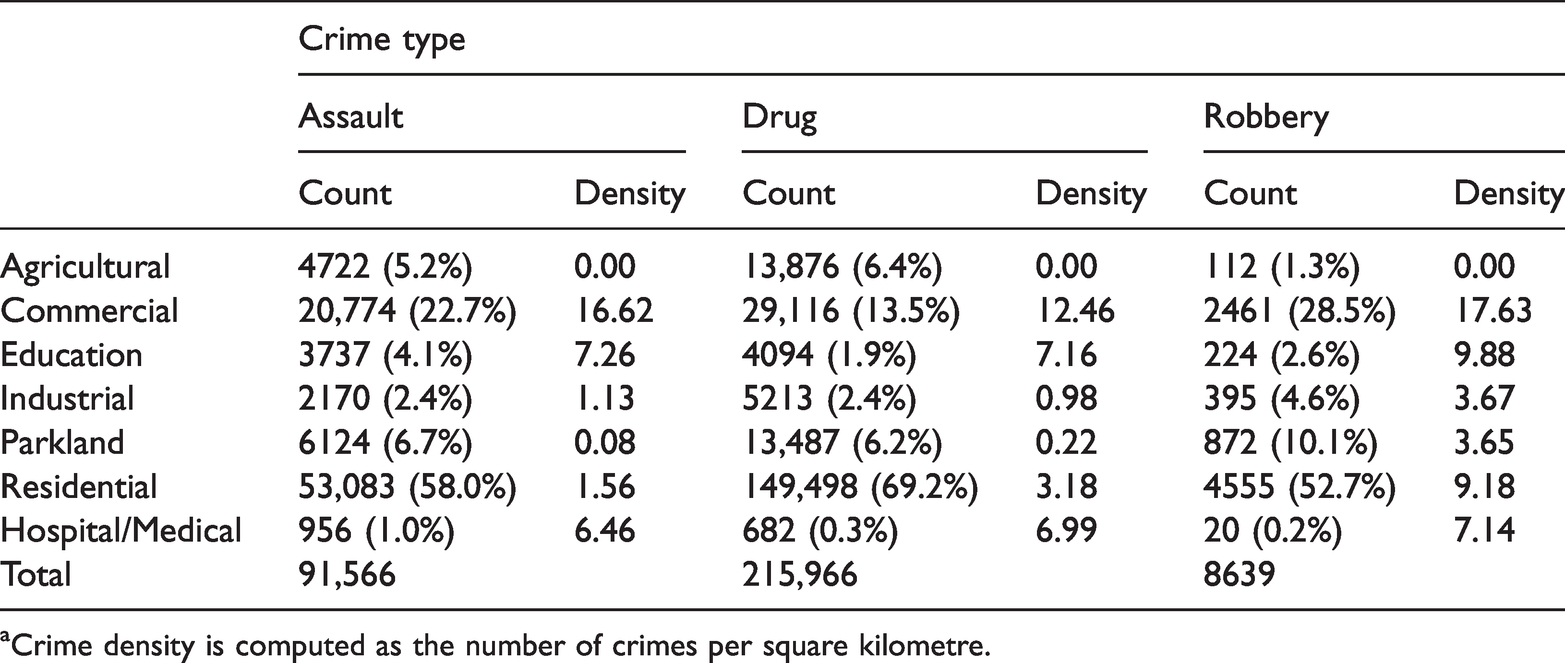
^aCrime density is computed as the number of crimes per square kilometre.

There are two components that comprise our analytic approach. We first employ Bertin plots (Bertin, 1977) as a visual analytic to describe how the timing of crime varies by land use. The Bertin plot describes what is essentially a numerical cross-tabulation, with the numerical values replaced by a symbol whose size reflects the value in each cell. The ordering of rows and columns, when not based on a natural progression such as hour in the day, can be chosen algorithmically. We select land use row ordering so that more similar time profiles are grouped together.

The second part involves modelling the output profiles via a variation on factor analysis. Assuming we model the cross-tabulation visualised in the Bertin plots, represented as a matrix $X$ such that

\log (E (X)) = W Z + e

(1)

where

X

is an m × n matrix (here m is the number of land uses and n is the number of time bins – i.e. 24), W is an

m \times k

matrix where

k < m, Z

is a

k \times n

matrix and

e

is an

m \times n

error term (usually we presume

e_{i j} \sim N (0, σ^{2}))

, and

X

is a matrix of integer counts corresponding to the cross-tabulations of time of day by land use type, and the counts are assumed to have a Poisson distribution, the logarithm of whose mean is given on the right-hand side of equation (1). The logarithm here is an element-by-element function, and expectations are also taken element by element for the rectangular m × n matrix X. Thus, the response for the regression model here is a matrix, rather than a column vector.

The

signals are the rows of

Z

and the multipliers are the columns of

W

. Note also that multiplying a row of

Z

by a constant and a column of

W

by the reciprocal of that constant gives identical results – and so here we adopt the convention that rows of

Z

are standardised to have a variance of 1.

In short, $Z$ can be regarded as $k$ ‘signals’ (one per hour over the 24-hour period) stacked in rows. The idea is like that of principal components – essentially each ‘signal’ is similar to principal component scores for each time bin in the day. The Poisson assumption is used here, as the crimes are assumed to be relatively rare events once they are disaggregated to hourly categories and crime type. The expected values refer to the averages over each given hour/type cell for all of the days in the study period. Without the logarithm transform, and the assumption that $X$ comprises Poisson counts the approach would be standard factor analysis – see, for example Mulaik (2010). $W$ composes the profile of each of the land use types by superimposing the signals together with different multipliers. $w_{i j}$ is the multiplier coefficient for signal $i$ in land use $j$ . The idea is that if $k$ is less than $m$ and reasonably small, then each signal can be given an interpretation, then seeing the multiplier coefficient for each land use helps to understand the underlying structure.

The key aspect of the Poisson adaptation here is to allow for the fact that in the observation space, the quantities observed are counts rather than continuous measurements. Thus, they can only be positive integers or zero. The logarithm transform, together with the Poisson distribution assumption allows for integer-valued observations, despite the fact that the underlying signals and multipliers are continuous values on the real line. The full model allows a replication of this network component (with a distinct ∑ unit) for each of the observed counts. A model of this form can be calibrated with the ‘PLNmodels’ R package (Chiquet et al., 2018, 2019). Here, the number k for each analysis is selected as the value minimising the bayesian information criterion (BIC) as outlined by Chiquet et al. (2018).

Results and discussion

Results are presented in two parts, beginning with a visual descriptive analysis of crime timing by land use before presenting results from the modelling exercise.

Figure 1 displays Bertin plots – these are designed so that crime types are ordered in a way that adjacent categories are more highly correlated. There is one plot for each of our three crime types – each with an appropriate ordering. As the three signals are orthogonal (i.e. uncorrelated), the ordering highlights the differing groupings of the crime types between the signals and emphasises the times at which that happens. These reveal that for assaults commercial areas are temporally concentrated and peak early afternoon, while industrial areas although less peaky experience assaults from the early hours of the morning through to around 14:00. Assault in education areas is a night-time phenomenon with a distribution spanning 22:00 to 05:00, whereas for parkland and residential areas this is from around 05:00 to 15:00. For drug crimes, the plot shows that residential, education and agricultural areas following a similar temporal pattern, that is night-time (commencing around 20:00) and continuing through to around 7 o’clock in the morning. Drug crimes in commercial, industrial, parkland, transport and medical/hospital areas commence a little later (around midnight) and continue through to around 14:00. For robberies, we restrict the Bertin plot to represent just six land use categories given the fewer number of incidents allied with their sparser distribution across land use. The visual show robbery to be broadly distributed across agriculture, education, parkland, industrial, commercial and residential places with a similar temporal signature commencing around 05:00 and dissipating by 17:00, thus a predominately day-time crime.

Figure 1.

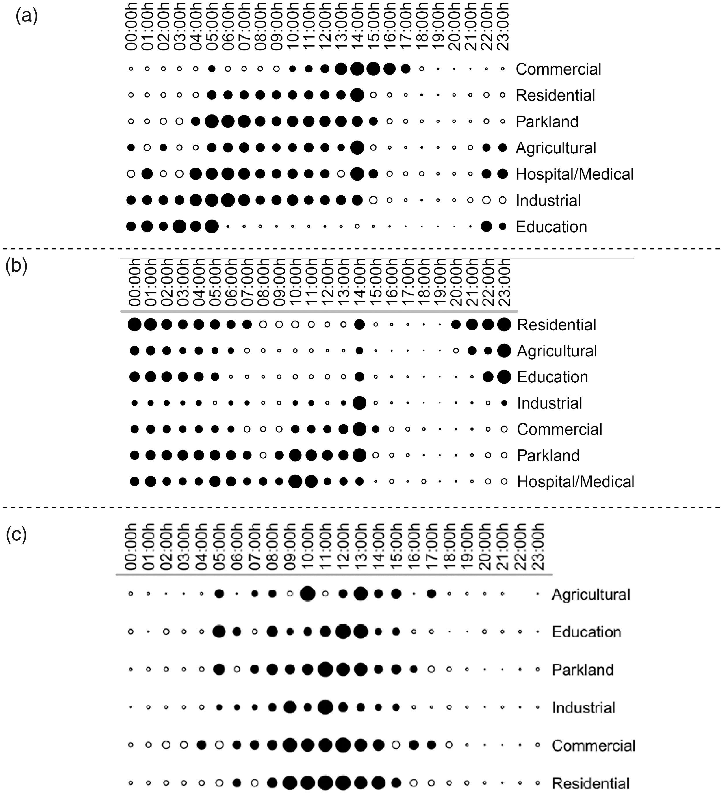
Bertin plots describing crime timing by land use for: (a) assault; (b) drug crime and (c) robbery.

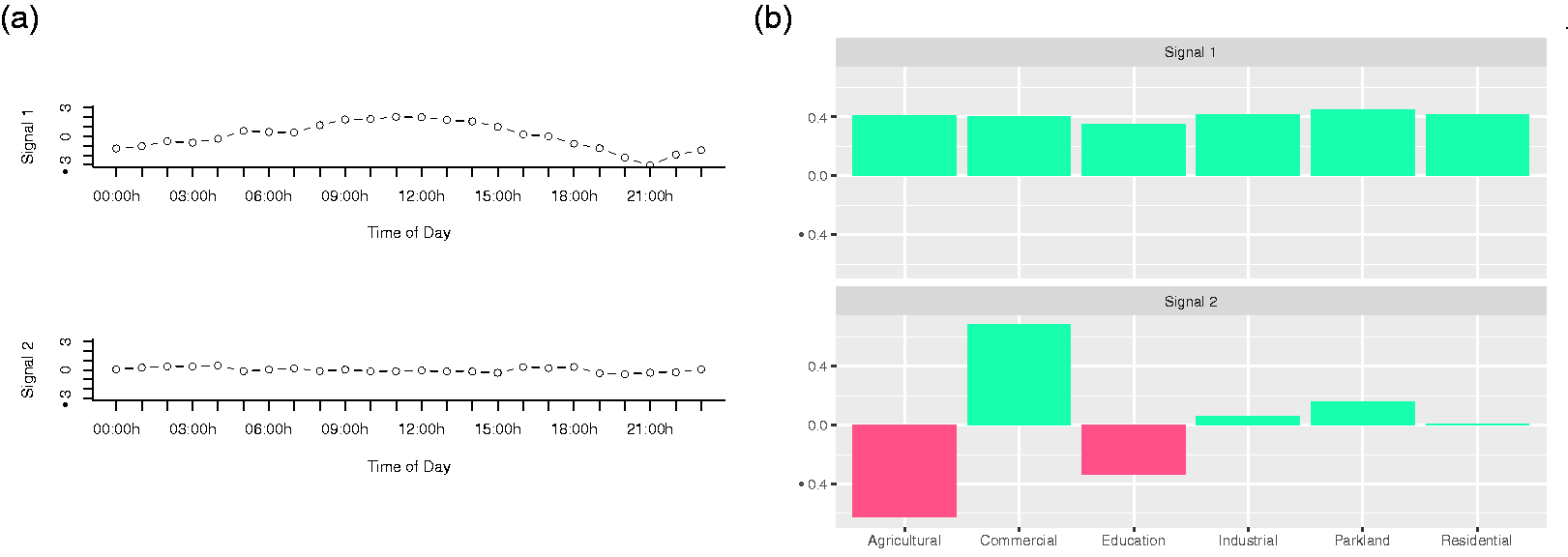
Next, we report results from the modelling exercise. To interpret the results, we will simultaneously draw on the information presented in Figures 2 to 4 reporting two outputs for each crime type: (a) the hourly signals and weights and (b) the multiplier values. More specifically, we look at the values represented in the vertical axis of the signals and multiplier plots to interpret the strength and direction of the effect at a given hour and its variation over the 24-hour period.

This is followed by next looking at the multiplier coefficients for each same signal to reveal how this effect is distributed across each land use category. These multipliers can have both positive and negative values. A positive value suggests that the number of events at a given hour for a given land use type is greater than on average for all land uses, whereas a negative value indicates the number below. As these signals and multipliers operate on a logarithmic scale, it is hard to interpret them directly and relative levels are more important. However, their estimates are available in Appendix 4. As such, through examining both the signals and weights along with their mixing values you can assemble a picture of how land use and crime is temporally distributed.

For assaults (Figure 2), BIC minimisation identified three distinct signals. The first signal has the most dominant effect on assaults (as denoted by the values in the vertical axis) and follows a relatively sustained high between around midnight and 14:00, dipping to a low at 19:00 before rising to a similar high as early at 22:00. The mixing values associated with signal one reveal that all land use types barring education (that has a mix that is double the magnitude of all other land use types) have a similar positive mix of this signal. The second signal is smaller in effect and follows elevated periods during night-time and early hours of the morning. The associated mixing values of signal two suggest that this signal is most only positively associated with the education land use, whilst all other land use categories experience less of signal two dynamics. The third signal exerts the smallest effect but reveals two main elevated periods, being the early hours of the morning (midnight to around 05:00) along with an afternoon peak (around 14:00 to 19:00). The mixing values of the third signal reveal on two land use types are positively associated with this dynamic, those being education and commercial. However, it is important to note that commercial has approximately twice the positive effect than that of education.

Figure 2.

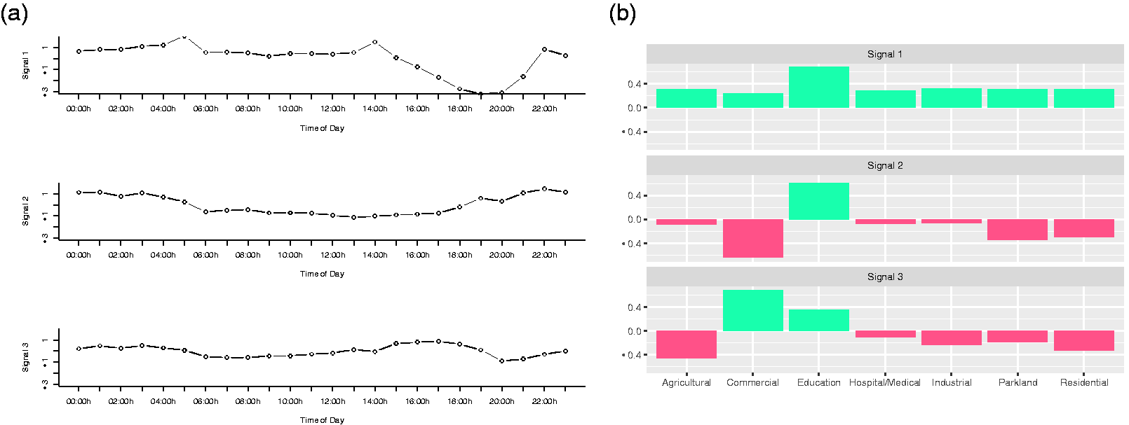
(a) Signals and (b) multiplier values for assaults.

For drug crimes (Figure 3), BIC also suggested three distinct signals. Common to that of assaults, the first signal has an elevated level from around midnight to around 14:00 in the afternoon, dipping to a low at 19:00 before rising to a commensurate high as early in the day by 23:00. Mixing values for signal one are positive for all land use types, but especially so for both agriculture and education that are approximately double in magnitude to that of commercial. The second signal is characterised by relatively low levels throughout the day and one peak around 20:00 in the evening. The mixing values indicate that only agriculture and residential have positive values, all other types, especially parkland and commercial are associated with negative values. Signal three has the smallest effect and follows a more complex distribution over the 24-hour period, with a peak during the early hours of the morning, a second around 18:00 and a final peak around 22:00. The mixing values for the third signal show that is just education that has a positive mix of this dynamic, all other land use types reporting relatively small negative associations.

Figure 3.

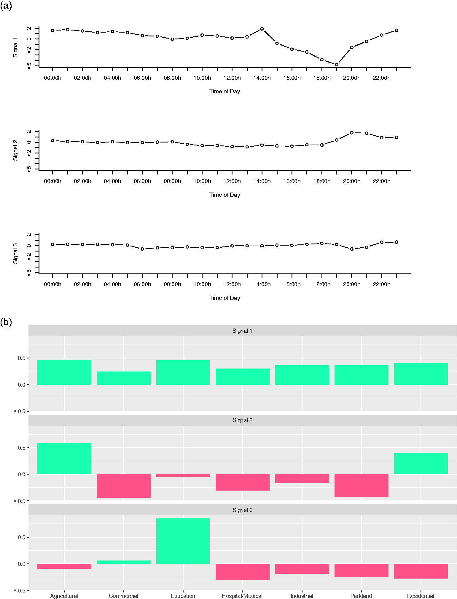
(a) Signals and (b) multiplier values for drug crime.

For robberies (Figure 4), BIC suggested that two distinct signals were identified in part relating to the fewer number of such incidents along with a greater degree of homogeneity in terms of their temporal dynamics across our different land use types (as highlighted in Figure 1(c)). Signal one shows a gradual rise with a peak around midday with mixing values that suggest all land use types have a more or less equal share of this dynamic. The second signal is more chaotic with peaks in the early hours of the morning (around 04:00) and another in late afternoon (around 16:00 to 18:00). Mixing values suggest that in the main part commercial areas and to a far lesser extent (but still positive) industrial, parkland and residential land uses experience this temporal signal.

Figure 4.

(a) Signals and (b) multiplier values for robbery.

Our results speak to the literature around risky places and risky times (Brantingham et al., 2020; Eck et al., 2007) in that we are able through our crime temporal signal methodology to establish clear and distinct differences between crime type and land use. In other words, crime is skewed both in the way it differentially impacts land uses but also in the timing of that crime risk. As such different types of crime are more prevalent in some land uses than others and that this relationship undergoes marked change over the course of a day. Thus, these finding align with those in the Corcoran et al. (2019) study that pointed to how commercial precincts can ‘flip’ from being crime free through much of the day to a hotspot of crime during a concentrated period of time.

Explanations for the observed patterning (in both space and time) can be drawn from three interrelated theories in environmental criminology, RAT (Cohen and Felson, 1979), crime pattern theory (Brantingham and Brantingham, 1993, 1995) and rational choice theory (Cornish and Clarke, 1986). These theories suggest that opportunities for crime are shaped by the diurnal mobility individuals as they go about their daily legitimate tasks and that these routines are governed by biological, social and employment needs. Crime will take place where there is a confluence in space and time of offenders and targets in situations where capable guardians are absent (RAT). Crime pattern theory talks to the way in which our individual activity spaces are both spatially and temporally bound and comprise a series of nodes (such as home and university) and are connected via a series of pathways. The familiarity of the places that fall within our activity spaces are familiar and it is this familiarity that gives rise to crime opportunities at our highly frequented nodes and along our pathways. Rational choice theory simply refers to the opportunity-cost trade-off a potential offender processes in a given locale at a given time wherein if opportunity outweighs costs, a crime is likely to occur.

In the context of land use and crime, our results echo the predictions of the three theories in that the diurnal redistribution of population gives rise to different crime opportunities at different times. Here, we observe that in residential areas assault is mostly experienced through the day, whereas for drug crime there is a night-time dimension to its distribution in the same land use type. Education areas experience both a day and a strong night-time propensity for assault a similar relationship for drug crimes and a daytime dynamic for robbery. Commercial areas experience an afternoon and night-time dynamic for assault and a night-time element for robbery. Taken together we can interpret these results in the light of temporary population movements where some crime types require the co-presence of other individuals/victims (i.e. assault and robbery) in which large population numbers are positively associated with crime risk, whereas drug crimes are located in places and at times which offer the least risk of detection, thus more likely negatively associated with population volume. This finding goes some way to highlight the need for a better empirical understanding of temporary populations and underscores the value of moving beyond simple ‘usual residence’-based denominators to measure crime incidence (Hanaoka, 2018; Hipp et al., 2019; Malleson and Andresen, 2015, 2016).

From a regional planning perspective our crime temporal signal methodology offers some benefits concerned with monitoring the crime–land use relationship. For example, deploying our method for a spatial subset of the data capturing the development itself and its immediate surrounding environs would enable an investigation of how planning decisions (such as the creation of a new regional shopping centre or the conversion of an inner city industrial area to a new residential space) might bring about shifts in crime timing and their mix across land use. In this example, segmenting the data set into two parts, one representing the ‘before’ and the second ‘after’ the development would enable a targeted evaluation of how the change in land use might be associated with changes in the temporal signals of crime. This capacity to monitor such shifts could be an important input to help ground smart land use planning decisions in both growing and shrinking regions (Browning et al., 2010; Frazier et al., 2013).

There are some limitations related to our input data and associated results that require noting. First relates to our unit of analysis, namely the MB. Despite this being the smallest geographic unit for which census data is released, some MBs can be both quite large (the largest being 21,713 square kilometres (the equivalent to the size of Israel), an agricultural area located in outback western Queensland) but also can include a small mix of land uses other than that captured by its primary classification – for a detailed description of the delimitation rules for MBs, see ABS (2016). Second, is the time recorded in the crime incident database. Whilst we have selected three crime types that research suggests should have more reliable time stamps – than a crime incident such as burglary where the lag between the incident occurring and being reported to the police can vary substantially (Ratcliffe, 2002) – there is the possibility that the temporal precision might not be consistently reliable. Given the lack of access to ancillary data via which we might attempt to triangulate crime timings (acknowledging that this is an extremely tricky task, although a promising study using Twitter data (Gerber, 2014) might point to a fruitful avenue for future research), we need to interpret the results with some caution around the issue of temporal precision.

Our crime temporal signal methodology presented here lays the foundation for a number of future research avenues. First, it would be interesting to reapply our method to specific aggregations of land uses in order to unpack the role played by land use mix on the observed number, timing and intensity of the crime signal. For example, this might include looking at commercial precincts that are spatially adjacent to an industrial areas and would follow established knowledge that land use mix is important in explaining variations in crime (Browning et al., 2010; Wo, 2019; Zahnow, 2018). This approach might be especially insightful in urban areas where MBs are far smaller and thus an individual’s activity space will cross-numerous land uses and also in which there will be multiple encounters with others over the course of a day. Second, given access to data that offers temporary population estimates at a fine spatial and temporal scale, an interesting follow-up study would be to use such estimates as a denominator and look at relative risk by land use given population present. This would permit us to explore the interplay between population present and crime opportunity and how this varies by crime type, land use and local socio-demographic and economic characteristics. Third would be conduction of cross-metropolitan and cross-national comparisons to test the extent to which the same temporal signal dynamics are detected and how situational and climatic contexts matter in shaping the crime–land use association.

Last, our approach makes a bold assumption of homogeneity of crime volume and timing within a given land use type and we know from scholarship that places considered the same by their land use classification may indeed have very different crime profiles – such as that by Corcoran et al. (2019) who highlight that commercial precincts that are located in close proximity to one another can experience crime both in quite dissimilar volumes and are distributed across a day and week differently. What would be an interesting follow-up study to that presented here would be to simply reapply our analytic approach to different categories of the same land use type, so for commercial precincts we might impose a sub-classification to differentiate between regional shopping centres, suburban strip malls and city centre precincts for example. Adopting this approach would then allow us to unpack the extent to which the commercial crime signal (presented here) is a function of a particular type of commercial precinct through analysing the way in which the signal mixes across the various commercial sub-categories.

Conclusion

In this paper, we presented our crime temporal signal method designed to delineate the assortment and contribution of temporal signals that explain the intensity of crime within and between particular land use types. This method moves beyond current methods that are concerned with examining crime timing and offers a number of important practical benefits for tactical policing and urban and regional planning. We also suggest that further understanding could be gained if the observed temporal patterns in a given crime type were considered in a spatiotemporal framework – for example considering whether profiles in temporal dynamics vary geographically or whether there is some form of spatial association between nearby patterns in different crime types. This is a topic we wish to prioritise in future work.

Footnotes

Declaration of conflicting interests

The author(s) declared no potential conflicts of interest with respect to the research, authorship, and/or publication of this article.

Funding

The author(s) received no financial support for the research, authorship, and/or publication of this article.

ORCID iD

Jonathan Corcoran

Note

Appendix 3. Crime type,by hour (South East Queensland)

South East Queensland (see inset map in Appendix 1) is the most populous region of Queensland wherein 72.5% of the State’s population usually reside (Queensland Government Statistician’s Office, 2020). This region is home to the State’s capital, Brisbane and accounts for 57% of our 3 crime types over the 5-year study period.

Appendix 4. Multiplier weights by crime type

Assault

Drug

Robbery

References

Andresen

Curman

Linning

(2017) The trajectories of crime at places: Understanding the patterns of disaggregated crime types. Journal of Quantitative Criminology 33(3): 427–449.

Australian Bureau of Statistics (2011a) Australian statistical geography standard (ASGS): Volume 1 – Main structure and greater capital city statistical areas (cat no. 1270.0.55.001). Available at: www.abs.gov.au/ausstats/abs@.nsf/Lookup/by%20Subject/1270.0.55.001∼July%202016∼Main%20Features∼Mesh%20Blocks%20(MB)∼10012 (accessed 28 January 2020).

Australian Bureau of Statistics (2011b) Australian statistical geography standard (ASGS) Volume 1 – Main structure and greater capital city statistical areas (cat no. 1270.0.55.00). Available at: www.abs.gov.au/AUSSTATS/abs@.nsf/DetailsPage/1270.0.55.001July%202011?OpenDocument (accessed 28 January 2020).

Australian Bureau of Statistics (2016) Australian statistical geography standard (ASGS): Volume 1 – Main structure and greater capital city statistical areas, July 2016 (cat no. 1270.0.55.001). Available at: www.abs.gov.au/ausstats/abs@.nsf/Lookup/by%20Subject/1270.0.55.001∼July%202016∼Main%20Features∼Mesh%20Blocks%20(MB)∼10012 (accessed 12 March 2021).

Bertin

(1977) La Graphique et le Traitement Graphique de L'information. Paris: Flammarion.

Bhaduri

Bright

Coleman

, et al. (2007) LandScan USA: A high-resolution geospatial and temporal modeling approach for population distribution and dynamics. GeoJournal 69(1–2): 103–117.

Boessen

Hipp

(2015) Close‐ups and the scale of ecology: Land uses and the geography of social context and crime. Criminology 53(3): 399–426.

Braga

Papachristos

Hureau

(2010) The concentration and stability of gun violence at micro places in Boston, 1980–2008. Journal of Quantitative Criminology 26(1): 33–53.

Brantingham

(1984) Patterns in Crime. New York: Macmillan.

10.

Brantingham

(1993) Environment, routine and situation: Toward a pattern theory of crime. Advances in Criminological Theory 5: 259–294.

11.

Brantingham

(1995) Criminality of place. European Journal on Criminal Policy and Research 3(3): 5–26.

12.

Brantingham

(2017) Notes on the geometry of crime. In: David Canter and Donna Youngs (eds) In: Principles of Geographical Offender Profiling. London: Routledge, pp.97–124.

13.

Brantingham

Song

, et al. (2020) Crime hot spots, crime corridors and the journey to crime: An expanded theoretical model of the generation of crime concentrations. In: Kim M. Lersch and Jayajit Chakraborty (eds), Geographies of Behavioural Health, Crime, and Disorder. Cham: Springer, pp.61–86.

14.

Browning

Byron

Calder

, et al. (2010) Commercial density, residential concentration, and crime: Land use patterns and violence in neighborhood context. Journal of Research in Crime and Delinquency 47(3): 329–357.

15.

Cahill

Mulligan

(2007) Using geographically weighted regression to explore local crime patterns. Social Science Computer Review 25(2): 174–193.

16.

Ceccato

Uittenbogaard

(2014) Space–time dynamics of crime in transport nodes. Annals of the Association of American Geographers 104(1): 131–150.

17.

Chiquet

Mariadassou

Robin

(2018) Variational inference for probabilistic Poisson PCA. The Annals of Applied Statistics 12: 2674–2698.

18.

Chiquet

Mariadassou

Robin

(2019) Variational inference for sparse network reconstruction from count data. In: Proceedings of the 36th international conference on machine learning, volume 97, 9-15 June 2019, Long Beach, California, USA. series: Proceedings of Machine Learning Research.

19.

Cohen

Felson

(1979) Social change and crime rate trends: A routine activity approach. American Sociological Review 44(4): 588–608.

20.

Cornish

Clarke

RVG

(1986) The Reasoning Criminal: Rational Choice Perspectives on Offending. New York: Springer-Verlag.

21.

Courtright

Mutchnick

(2002) Cartographic school of criminology. In: Levinson

(ed.) Encyclopedia of Crime and Punishment. Thousand Oaks, CA: Sage, pp.175–177.

22.

Corcoran J, Zahnow R, Kimpton A, Wickes R and Brunsdon C (2021) The temporality of place: Constructing a temporal typology of crime in commercial precincts. Environment and Planning B: Urban Analytics and City Science 48(1): 9–24.

23.

Eck

Clarke

Guerette

(2007) Risky facilities: Crime concentration in homogeneous sets of establishments and facilities. Crime Prevention Studies 21: 225.

24.

Felson

Boivin

(2015) Daily crime flows within a city. Crime Science 4(1): 31.

25.

Frazier

Bagchi-Sen

Knight

(2013) The spatio-temporal impacts of demolition land use policy and crime in a shrinking city. Applied Geography 41: 55–64.

26.

Gerber

(2014) Predicting crime using twitter and kernel density estimation. Decision Support Systems 61: 115–125.

27.

Groff

(2010) Quetelet, Adolphe: Explaining crime through statistical and cartographic techniques. In: Cullen FT and Wilcox P (eds) Encyclopedia of Criminological Theory. Sage Publications,Thousand Oaks, California, 748-753.

28.

Groff

(2014) Quantifying the exposure of street segments to drinking places nearby. Journal of Quantitative Criminology 30(3): 527–548.

29.

Groff

Weisburd

Yang

(2010) Is it important to examine crime trends at a local “micro” level? A longitudinal analysis of street to street variability in crime trajectories. Journal of Quantitative Criminology 26(1): 7–32.

30.

Grubesic

Mack

(2008) Spatio-temporal interaction of urban crime. Journal of Quantitative Criminology 24(3): 285–306.

31.

Hanaoka

(2018) New insights on relationships between street crimes and ambient population: Use of hourly population data estimated from mobile phone users’ locations. Environment and Planning B: Urban Analytics and City Science 45(2): 295–311.

32.

Hipp

Bates

Lichman

, et al. (2019) Using social media to measure temporal ambient population: Does it help explain local crime rates? Justice Quarterly 36(4): 718–748.

33.

Hodgkinson

Andresen

(2019) Changing spatial patterns of residential burglary and the crime drop: The need for spatial data signatures. Journal of Criminal Justice 61: 90–100.

34.

Johnson

Bernasco

Bowers

, et al. (2007) Space–time patterns of risk: A cross national assessment of residential burglary victimization. Journal of Quantitative Criminology 23(3): 201–219.

35.

Kimpton

Corcoran

Wickes

(2017) Greenspace and crime: An analysis of greenspace types, neighboring composition, and the temporal dimensions of crime. Journal of Research in Crime and Delinquency 54(3): 303–337.

36.

Kinney

Brantingham

Wuschke

, et al. (2008) Crime attractors, generators and detractors: Land use and urban crime opportunities. Built Environment 34(1): 62–74.

37.

Knox

(1964) Epidemiology of childhood leukaemia in Northumberland and Durham. British Journal of Preventive & Social Medicine 18(1): 17.

38.

Kurland

Johnson

(2019) The influence of stadia and the built environment on the spatial distribution of crime. Journal of Quantitative Criminology 37: 573–604.

39.

Kurtz

Koons

Taylor

(1998) Land use, physical deterioration, resident-based control, and calls for service on urban streetblocks. Justice Quarterly 15(1): 121–149.

40.

Leffondré

Abrahamowicz

Regeasse

, et al. (2004) Statistical measures were proposed for identifying longitudinal patterns of change in quantitative health indicators. Journal of Clinical Epidemiology 57(10): 1049–1062.

41.

Malleson

Andresen

(2015) Spatio-temporal crime hotspots and the ambient population. Crime Science 4(1): 10.

42.

Malleson

Andresen

(2016) Exploring the impact of ambient population measures on London crime hotspots. Journal of Criminal Justice 46: 52–63.

43.

Mulaik

(2010) Foundations of factor analysis. 2nd ed. Boca Raton, FL: CRC Press.

44.

Nagin

Land

(1993) Age, criminal careers, and population heterogeneity: Specification and estimation of a nonparametric, mixed Poisson model. Criminology 31: 327–362.

45.

Newton

(2004) Crime on public transport: ‘Static’ and ‘Non-Static’ (moving) crime events. Western Criminology Review 5(3): 25–42.

46.

Nielsen

Rosenthal

Sun

, et al. (2014) Group-based criminal trajectory analysis using cross-validation criteria. Communications in Statistics – Theory and Methods 43(20): 4337–4356.

47.

Parker

McCall

(1999) Structural conditions and racial homicide patterns: A look at the multiple disadvantages in urban areas. Criminology 37(3): 447–478.

48.

Phillips

Cochrane

(1988) Crime and Nuisance in the Shopping Centre: A Case Study in Crime Prevention. London: Home Office, p.16.

49.

Queensland Government Statistician’s Office (2020) Population growth highlights and trends, Queensland regions, 2020 edition. Available at: www.qgso.qld.gov.au/issues/3061/population-growth-highlights-trends-qld-regions-2020-edn.pdf (accessed 13 March 2021).

50.

Quetelet

LAJ

(1842) A Treatise on Man and the Development of His Faculties. Cambridge: Cambridge University Press.

51.

Quick

Law

(2019) Time-varying relationships between land use and crime: A spatio-temporal analysis of small-area seasonal property crime trends. Environment and Planning B: Urban Analytics and City Science 46(6): 1018–1035.

52.

Ratcliffe

(2002) Aoristic signatures and the spatio-temporal analysis of high volume crime patterns. Journal of Quantitative Criminology 18(1): 23–43.

53.

Ratcliffe

(2004) The hotspot matrix: A framework for the spatio‐temporal targeting of crime reduction. Police Practice and Research 5(1): 5–23.

54.

Roncek

Maier

(1991) Bars, blocks, and crimes revisited: Linking the theory of routine activities to the empiricism of “hot spots”. Criminology 29(4): 725–753.

55.

Shaw CR and McKay HD (1942) Juvenile delinquency and urban areas. University of Chicago Press.

56.

Smith

Newing

Quinn

, et al. (2015) Assessing the impact of seasonal population fluctuation on regional flood risk management. ISPRS International Journal of Geo-Information 4: 1118–1141.

57.

Stucky

Ottensmann

(2009) Land use and violent crime. Criminology 47(4): 1223–1264.

58.

Sutherland

Cressey

(1978) Criminology. 10th ed. Philadelphia, PA: Lippincott.

59.

Sylvestre

McCusker

Cole

, et al. (2006) Classification of patterns of delirium severity scores over time in an elderly population. International Psychogeriatrics 18(4): 667–680.

60.

Taylor

Haberman

Groff

(2019) Urban park crime: Neighborhood context and park features. Journal of Criminal Justice 64: 101622.

61.

Townsley

Grimshaw

(2013) The consequences of queueing: Crowding, situational features and aggression in entertainment precincts. Crime Prevention and Community Safety 15(1): 23–47.

62.

Valente

(2019) Spatial and temporal patterns of violent crime in a Brazilian state capital: A quantitative analysis focusing on micro places and small units of time. Applied Geography 103: 90–97.

63.

Weisburd

Bushway

Lum

, et al. (2004) Trajectories of crime at places: A longitudinal study of street segments in the city of Seattle. Criminology 42(2): 283–322.

64.

Weisburd

Bruinsma

Bernasco

(2008) Units of analysis in geographic criminology: Historical development, critical issues and open questions. In: Weisburd

Bernasco

Bruinsma

(eds) Putting Crime in Its Place: Units of Analysis in Spatial Crime Research. New York: Springer-Verlag, pp.3–31.

65.

Wheeler

(2019) Quantifying the local and spatial effects of alcohol outlets on crime. Crime & Delinquency 65(6): 845–871.

66.

Wheeler

Worden

McLean

(2016) Replicating group-based trajectory models of crime at micro-places in Albany, NY. Journal of Quantitative Criminology 32(4): 589–612.

67.

(2019) Mixed land use and neighborhood crime. Social Science Research 78: 170–186.

68.

Zahnow

(2018) Mixed land use: Implications for violence and property crime. City & Community 17(4): 1119–1142.

69.

Zahnow

Corcoran

(2019) Crime and Bus Stops: An Examination Using Transit Smart Card and Crime Data. Environment and Planning B: Urban Analytics and City Science.