
Abstract
The general transit feed specification is becoming a popular data format for the publication of public transport schedules, making possible the collection of a nation-wide public transport schedule dataset, which enables monitoring of transit supply at an up-to-date and more precise level across a country than previously possible. In this paper, we use general transit feed specification data to measure local-scale public transport availability across England based on service frequency and spatial proximity to public transport stops/stations. Moreover, to demonstrate the usefulness of public transport availability measures, we examine inequalities of public transport provision and identify areas at risk of transport poverty across England. Furthermore, we estimate population (number of households) who are likely to suffer from transport poverty, accounting for public transport availability, time-based job accessibility by public transport or walking, household income and car ownership levels. Based on the criteria, we have used to identify public transport risk, we find that investment in the development of public transport services should prioritise West Midlands, East of England, South East and South West as those regions have more households who are likely to suffer from transport poverty. This paper contributes by (1) defining more comprehensive transit availability measures than existing measures at a variety of geography levels and (2) integrating fours aspects (i.e. public transport availability, job accessibility by public transport or walking, household income and car availability) to analyse transport poverty comprehensively.
Keywords
Introduction
Transport accessibility refers to the access to key services or destinations, such as employment, healthcare, education, recreation and shopping, etc. travel times to key services or destinations are conventionally used as measures of transport accessibility. Transport accessibility is further classified by transport mode, i.e. travel times to key amenities by public transport, travel times to key amenities by car, travel times to basic amenities by walking and travel times to key amenities by cycling. Apart from these rudimental metrics, the slightly more complex gravity models derived from social physics have also seen a fair number of applications in the measures of transport accessibility (Neutens, 2015). Considering destination sizes, gravity measures permit the incorporation of spatial interaction mechanisms (Neutens, 2015). However, gravity-based accessibility measures cannot be interpreted easily (Liu and Zhu, 2004). Unlike transport accessibility dedicated to quantifying the access to basic amenities (journey times to amenities), transport availability refers to the level of transport service provision (access to transport services). More specifically, private transport availability takes account of car ownership, car affordability and access to parking; whilst public transport availability takes account of proximity to stations/stops and frequency assuming the majority of people afford to use public transport services on a daily basis. Job accessibility by public transport (travel times to employment centres by public transport) is often used to represent the level of transport accessibility, as commuting is the most important travel purpose and public transport is the most important transport mode for the majority of residents. Although time-based transport accessibility indicators (e.g. travel time by public transport to nearest basic amenities) might be more useful in some applications, transport availability indicators have two advantages over time-based transport accessibility indicators. First, unlike transport accessibility measures, transport availability measures are usually independent of the locations of basic amenities. Public transport availability measures can be more easily measured and updated than transport accessibility measures by public transport as the lack of locations of basic amenities cannot affect the measures of public transport availability. Second, public transport availability measures can be areal-level (small area-level) or point-level (station/stop-level) measures; whilst transport accessibility measures are only areal-level (small area-level) measures.
Equity has been a major concern motivating the provision of public transport in regional and urban planning (Delbosc and Currie, 2011). Low-income people are likely to rely on public transport (i.e., bus, tram, subway, ferry and train) as an affordable means of travel, although there are variations in the usage of public transport between income groups. For instance, in the UK, more bus and walking trips are made by the lowest income group than any other group whereas more rail and bicycle trips are made by those from high-income group than others (Titheridge et al., 2014). Relevant studies have revealed that public transport availability is likely to impact employment of low-income people. For instance, proximity to public transport stations/stops is associated with large, statistically significant gains in accessibility to low-wage jobs (Fan et al., 2010; Thakuriah and Metaxatos, 2000). Low-income people living in areas with limited public transport availability are more likely to benefit from improvements in public transport services than people living in other areas. Areas where there are low-income people experiencing limited (public and private) transport availability are likely to be areas of high levels of social inequity. The identification of such areas would support the development of place-based strategies involving targeted investment in public transport.
Unlike income and car availability, the extent of public transport availability (in terms of service quality and coverage) is not directly available in Census data or household travel surveys. Although some studies simply use spatial proximity to stations/stops to measure public transport availability, it has been widely accepted that public transport availability is a broad concept. Public transport availability could be measured with multiple variables including the number of public transport stops (stations) in each neighbourhood, the number of routes, frequency of service, transfer times, proximity to public transport stops (stations) and others (Wells and Thill, 2012). Aside from service-based measures, public transport availability can also be measured within a spatial interaction model framework, where aside from availability and impedance to destinations, the opportunities and competition available for resources to travellers at destinations (for jobs, healthcare etc.) are also accounted for (Kawabata and Shen, 2006; Sen et al., 1999).
In this study, we aim to bridge three research gaps. First, although public transport availability has been measured using schedule data in some European, American and Australian regions or cities (e.g. Delbosc and Currie, 2011; Fransen et al., 2015; Pyrialakou et al., 2016), country-wide public transport availability measures combining spatial proximity and service frequency have not been produced or mapped. Adopting the transit availability measures of Minocha et al. (2008), this study attempts to measure local-scale public transport availability (public transport provision level) combining spatial proximity and service frequency throughout England, using emerging forms of data (i.e. general transit feed specification (GTFS) data). Second, most of the existing studies used a circular buffer to delineate the service area of stop/station whilst a road network buffer could make more sense. In this study, we replace a circular buffer with a road network buffer to accurately delineate the service area of a stop/station. Third, local-scale transport poverty at a larger geographical scale was rarely discussed in the existing studies. Although some studies examined the transport poverty in the UK, they neglected to examine spatial inequalities of transport poverty (Lucas et al., 2018; Mattioli et al., 2018; Sustrans, 2013). In this study, we attempted to examine local-scale transport poverty risk across a country based on public transport availability, job accessibility by public transport or walking, household income and car availability. Compared with a previous study which accounts for three aspects: income, distance to station/stop and distance to basic amenities (Sustrans, 2013), this study enhances the public transport provision aspect by replacing purely distance-based measures with one combining distance and service frequency. Besides, we integrate car availability as a new aspect into the measures of transport poverty risk. Owing to the availability of public transport schedule data, we attempt to examine spatio-social inequalities of transit provision and identify areas at risk of transport poverty across England.
Specifically, in this study, we first use GTFS data to measure public transport availability combining spatial proximity and service frequency, and then map public transport availability across England. Second, to demonstrate the usefulness of local-scale public transport availability measures, we attempt to use public transport availability measures to identify areas at risk of transport poverty across England. To help reduce socio-spatial inequalities of public transport availability effectively, we examine population (households) at risk of transport poverty according to a combination of public transport availability, job accessibility (travel time) by public transport or walking, income level and car availability. One contribution of the paper is to automate the process for capturing the data on an ongoing basis so as to create a longitudinal dataset that would be invaluable to monitoring public transport quality including seasonality and other temporal dynamics, in addition to spatial and network coverage, over time. Another contribution of the paper is to perform an investigation of transport poverty risk at a larger geographical scale, which is a good example of demonstrating the usefulness of public transport availability measures. Moreover, this paper makes contributions to the methodological development by (1) defining more comprehensive transit availability measures than existing measures at a variety of geography levels and (2) integrating fours aspects (i.e. public transport availability, job accessibility by public transport or walking, income and car availability) to identify transport poverty risk comprehensively.
Background and motivations
Public transport availability
Social exclusion in transport has been extensively studied (Lucas, 2012; Preston and Raje, 2007; Schwanen, et al., 2015; Social Exclusion Unit, 2003), pointing to the barriers imposed by lack of affordable and reliable transport to economic and social outcomes (Blumenberg and Pierce, 2016; Sanchez, 2008; Widener et al., 2015). Public transport plays a vital role in the daily life of people who own no private vehicles or cannot afford a car. Levels of public transport availability affect the usage of public transport, including usage desire and frequency. An accurate measure of public transport availability could enhance the demand and supply analysis for public transport services. Earlier studies measured purely proximity-based public transport availability, considering the number of public transport stops in the local area, or proximity to public transport stops (Fan et al., 2010); whilst in the last two decades some studies have attempted to measure public transport availability by combining spatial proximity and service frequency, including the number of routes and frequency of service, which have provided a more complete and realistic picture of public transport availability (Currie, 2010; Eboli and Mazzulla, 2012; Fu and Xin, 2007; Lovett et al., 2002; Mamun and Lownes, 2011; Mavoa et al., 2012; Mondou, 2001; Polzin et al., 2002; Rood, 1998; Ryus et al., 2000; Wu and Hine, 2003; Xu et al., 2015; Yigitcanlar et al., 2008; ). Using public transport availability to represent the level of public transport provision, researchers have attempted to evaluate public transport equity within cities or evaluate public transport equity in a city as a whole (Delbosc and Currie, 2011; Ricciardi et al., 2015; Rock et al., 2016; Shirmohammadli et al., 2016). Other researchers have attempted to identify areas of ‘high need–low provision’ in Asian, American, and Australian cities (Currie, 2010; Duvarci et al. 2015; Fransen et al., 2015; Jaramillo et al., 2012). Specifically, they identified spatial gaps in public transport provision for people who are socially disadvantaged, including those who are low income, unemployed, and without further or higher education. The vast majority of the earlier studies performed city-level or region-level analyses and focused on public transport equity in specific areas (Currie, 2010; Duvarci et al. 2015; Fransen et al., 2015; Goodman, 2013; Jaramillo et al., 2012; Pyrialakou et al., 2016; Rae, 2016). There is limited analysis on the level of public transport availability and deprived communities experience at the scale of an entire country. Being able to do so would be important to identify gaps accurately. For many country-level analyses of transport demand and use patterns, the major source of data is usually the decennial census. In very recent years, new forms of data collected from widely instrumented and crowdsourced systems open up the ability to assess transport quality at more localised levels and more frequently compared to the census or survey data. As a user-friendly data format, GTFS, is becoming the most popular format to publish public transport schedules (Farber and Fu, 2017; Fransen et al, 2015; Owen and Levinson, 2017). GIS techniques enable researchers to use GTFS data in measuring and mapping local-scale transport availability. To comprehensively measure public transport availability, Minocha et al. (2008) developed a suite of ‘public transport availability indices’, including service frequency, hours of service and service coverage. Similarly, other researchers measured public transport availability by walking distance to stations/stops and service frequency (Currie, 2010; Delbosc and Currie, 2011). Furthermore, Minocha et al. (2008) proposed a weighted Public Transport Availability Index (PTAI) by assigning different weights to service frequency in different time slots (e.g. peak time vs. off-peak time). This study improves the approach of Minocha et al. (2008) by (1) replacing a circular buffer with a road network buffer and (2) replacing hourly weights based on hourly distribution of real trips with hourly weights based on hourly distribution of estimated trips.
Transport poverty
Since 2008 public transport support from central and local governments in the UK has been decreasing (UK Department for Transport, 2016). Between 2009/2010 and 2013/2014, supported service mileage of the UK bus network is estimated to had fallen by around 22% in metropolitan areas and 24% in non-metropolitan areas (UK Department for Transport, 2016). According to a recent report, in England nearly 1.5 million people are at high risk of suffering from ‘transport poverty’ (Sustrans, 2013). Transport poverty is a complex issue and is therefore inherently difficult to accurately measure (Sustrans, 2013). Although there is no official recognition of transport poverty yet (Lucas et al., 2016), the report combines three aspects of ‘transport poverty’: areas of low income (where the costs of running a car would place a significant strain on household budgets); areas where a significant proportion of residents live more than a mile from their nearest bus stops or railway stations and areas where it takes over an hour to access essential goods and services by walking, cycling or public transport (Sustrans, 2013). As a result, areas in England are identified as facing ‘low’, ‘medium’ or ‘high’ risk of transport poverty. Accordingly, nearly 1.5 million English people are at high risk of suffering from transport poverty (Sustrans, 2013). However, they some key aspects, such as the car access and public transport service quality (frequency or punctuality), in the definition of transport poverty. Some studies offer empirical findings to corroborate that people who has no private vehicles rely more on public transport (Badland et al., 2010; Matas et al., 2009). Low-income households or no-car households are likely to suffer from transport poverty risk. Although living in the areas with a low average income, households who are not in low income or afford to use a car are not at high risk of suffering from transport poverty. Like walking distance to the nearest stop/station, service frequency of the nearest stop/station also affects residents’ desire to use public transport. Use of walking distance to the nearest stop/station alone as the measure of public transport availability is simple and of bias. Furthermore, although some other studies had examined transport poverty risk in the UK, they either lacked national analysis (Lucas et al., 2018; Mattioli et al., 2018). This study aims to perform an analysis of transport poverty risk at a larger geographical scale.
Research approach and methods
We first present how to measure public transport availability at the small area levels. After that, we briefly introduce how to identify areas at risk of transport poverty and estimate population who are likely to suffer from transport poverty. In addition, the research data, including the GTFS data, job accessibility data, income data, car availability data and so forth, are introduced.
Data
In this section, the data used are introduced. Table 1 shows the description of the datasets used in this study. The details of the datasets are presented in the supplementary material.
Description of the datasets used in this study.
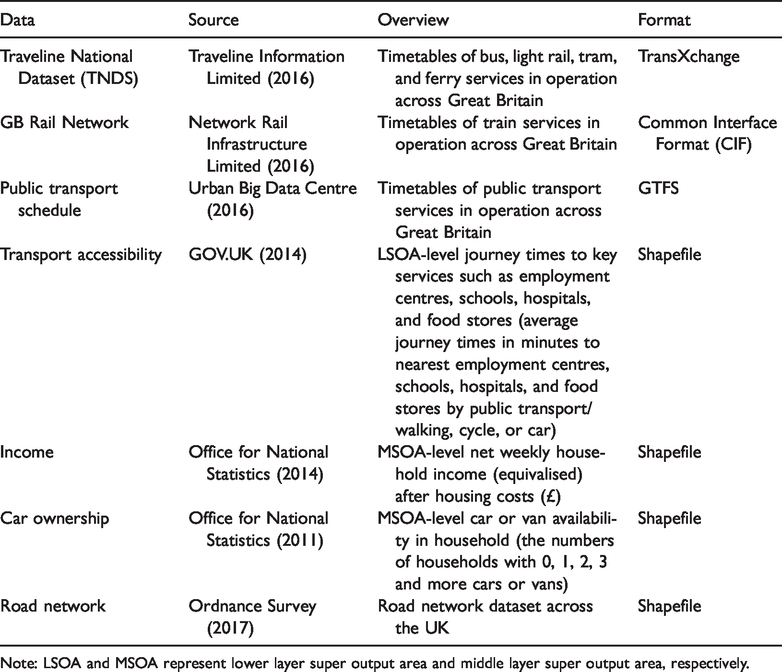
Note: LSOA and MSOA represent lower layer super output area and middle layer super output area, respectively.
Measures of public transport accessibility
In the suite of GTFS datasets, ‘stations.csv’ offers the locations and types of the stations/stops, whilst ‘routes.csv’ and ‘trips.csv’ offer the routes and service times of the stations/stops.
Calculation of stop-level PTAI
Adopting the transit availability measures of Minocha et al. (2008), we used the weighted PTAI to represent public transport availability at the stop/station level. Compared to Minocha et al. (2008), we determine the hourly weights according to hourly distribution of trips in England. Weights of service hours are proportional to the number of trips in progress within hours as we assume that high demand of trips within an hour means high importance of that hour. A larger number of trips in one hour means that hour is more likely to be a peak time period, during which each train or bus is likely to serve more people. In other words, that hour is likely to play a larger role in public transport services. The UK National Travel Survey offers hourly number of trips in progress on workdays in England for 2015 (Monday to Friday) (GOV.UK, 2013).
In this study, we focus on public transport availability on workdays as the majority of trips to basic destinations, such as workplaces and schools, only occur on workdays. Public transport availability on workdays reflects to what extent public transport can serve people and support their basic activities. The weighted PTAI is the weighted hourly number of trips passing a station (stop) on five workdays (Monday to Friday). Suppose i is a stop/station, its weighted PTAI is calculated as
Aggregation of stop-level PTAI to MSOA
As middle layer super output areas (MSOAs) and lower layer super output areas (LSOAs) are widely used to improve the reporting of small area statistics in England and Wales, the majority of socio-economic datasets are provided at these levels. MSOAs are built from groups of contiguous LSOAs. Typically, the average population of MSOAs is 7200, whilst that of LSOAs is 1500. There are now 34,753 LSOAs and 7201 MSOAs in England and Wales (Office for National Statistics, 2015). The population and household count of LSOA range from 1000 to 3000 and from 400 to 1200, whilst the population and household count of MSOA ranges from 5000 to 15,000 and 2000 to 6000. As income and car availability information is available at the MSOA level, we aggregate stop-level PTAIs to MSOAs to ensure PTAI is linkable to income and car availability information at the same geography level. Accordingly, the MSOA-level PTAI is used to represent the MSOA-level public transport availability in this study. To accurately measure PTAI for each MSOA, we take account of both the service levels and service areas of stations/stops.
First, service areas of stations/stops are generated. The service area is the area within which people are willing to walk to the station/stop. There is a declining tendency for patrons to access a bus service as walking distance to a bus stop increases (Langford et al., 2012). Conventionally, a circular buffer centred on a station/stop is used to simply represent the service area of the station/stop. Recently it has been recommended that a road network buffer should be used instead of a circular buffer to accurately measure access level (walking distance) along road network. Compared to Minocha et al. (2008), we choose road network buffers instead of circular buffers to accurately delineate service areas of stations/stops. Unlike circular buffers, road network buffers are irregularly shaped. A road network buffer of a station/stop is the area where walking distance to station/stop the along the road network is no larger than acceptable maximum walking distances. Some studies suggest acceptable maximum walking distances for public transport modes (Currie, 2010; Delbosc and Currie, 2011; Langford et al., 2012), and these are the distances that 75–80% of people would walk to access a stop/station according to a travel survey (Parsons et al., 2003): Access to bus stop = 400 m. Access to tram stop = 400 m. Access to rail station = 800 m. Access to ferry station = 800 m.
Next, we overlap service areas of stations/stops with LSOAs. Since the buffers of some stops overlap with that of others, the overlapping areas are served by more than one stop (see Supp Fig 1). Additionally, although some stations/stops are not situated in a LSOA, their buffers partly overlap LSOAs (see Stop 2 in Supp Fig 1). Considering these two issues, we overlap each station/stop’s buffer with LSOAs to know which LSOA is served by which stations/stops. In Supp Fig 1, the LSOA a is served by Stop 1, Stop 2, Stop 3, Stop 4 and Station 1. For simplicity, we use the regularly shaped buffers (circular buffers) to represent irregularly shaped buffers (road network buffers) in reality in Supp Fig 1.
After that, we are able to aggregate stop-level PTAI to LSOA. A combined measure of service level (hourly service frequency) and access distance is then calculated for each LSOA. Suppose a is a LSOA, its PTAI is calculated as
Finally, we incorporate population into the aggregation of LSOA-level PTAI to MSOA. Since population density is not evenly distributed among LSOAs within a MSOA, aggregating LSOA-level PTAI to MSOA by a population-weighted method should be better than by an area-populated method. Therefore, a population-weighted PTAI is then calculated for each MSOA. Suppose A is a MSOA, its PTAI is calculated as
Risk of transport poverty
In this study, we examine the risk of transport poverty by identifying the areas with a low level of PTAI and a low level of job_accessibility simultaneously. As a time-based measure, job_accessibility alone might be used to assess transport poverty risk. However, job_accessibility measures used are represented by journey times to the nearest employment centres rather assuming people are likely to work in the nearest employment centres. In fact, some people do not work in the nearest employment centres, gaps between modelled job_accessibility and realistic job_accessibility exist for some people. As only using job_accessibility to assess transport poverty risk is likely to have limitations and bias, using job_accessibility and public transport availability simultaneously to assess transport poverty risk is preferred. Since a household is deemed to be in poverty if the household’s income lies below 60% of the UK median income (Office for National Statistics, 2017), we used 60% of the median as the threshold for other indicators in this study as well. Specifically, a MSOA is considered in a low level of PTAI if its PTAI value lies below 60% of the median PTAI of England; and an MSOA is considered in a low level of job_accessibility if its time_to_workplace value lies above 1.5 times of the median time_to_workplace of England (note: 1.5 is close to the reciprocal of 60%). As a consequence, the areas at risk of transport poverty across England will be identified. It is noted that Wales is excluded because the job accessibility data for Wales is not available. Lately, we attempt to estimate population (number of households) suffering from transport poverty by counting households in income poverty and no-car households in the areas of high transport poverty risk. Of households in the areas of high transport poverty risk, those in income poverty or no-car households are likely to suffer from transport poverty.
Results and discussions
This section demonstrates the computed PTAI levels and identified areas at high risk of transport poverty across England. Note that Scotland and Wales are not considered in the identification of areas at high risk of transport poverty as they are not covered by the transport accessibility data.
Calculation of PTAI
First, we calculated stop-level PTAI by equation (1). This is followed by aggregating PTAI from stops/stations to MSOAs based on equations (2)–(3).
Identifications of transport poverty risk
We further attempt to estimate population (number of households) who are likely to suffer from transport poverty by counting households in income poverty and no-car households in the areas of high transport poverty risk. Of households in the areas of high transport poverty risk, those in income poverty or no-car households are likely to suffer from transport poverty.
First, we examine the areas at risk of transport poverty across England. We produce a map on which all the English MSOAs are classified into ‘low levels of PTAI’ and ‘non-low levels of PTAI’; and then produce another map on which all the English MSOAs are classified into ‘low levels of job_accessibility’ and ‘non-low levels of job_accessibility’. We overlay those two maps, and then identify the areas labelled as ‘low levels of PTAI’ and ‘low levels of job_accessibility’ simultaneously as ‘areas at high risk of transport poverty’. As a result, there are 350 English MSOAs are identified as the areas of high transport poverty risk (see Supp Fig 2). And there are approximately 1.1 million households living in those areas, accounting for approximately 5% of the households in England.
Second, we estimate the population (the number of households) who are likely to suffer from transport poverty by counting households in income poverty and no-car households in the areas of high transport poverty risk. As a result, among those living in the areas of high transport poverty risk, approximately 194,000 households are in income poverty and 173,000 households have no private vehicles. As the number of households in income poverty and having no private vehicles simultaneously are unknown, the number of English households who are likely to suffer from transport poverty is estimated between 194,000 and 367,000.
Furthermore, we compare transport poverty risk between regions across England. Supp Tab 1 shows the count and percent of households in income poverty and no-car households living in the areas of high transport poverty risk at the regional scale. In Supp Tab 1, C_HIP, C_NCH, P_HIP, and P_NCH are the count of households in income poverty, the count of no-car households, the percent of households in income poverty and the percent of no-car households living in the areas of high transport poverty risk. P_HIP is equal to C_HIP/population (count of households) in a region; and P_NCH is equal to C_NCH/population (count of households) in a region. West Midlands, East of England, South East and South West all rank the top 5 by C_HIP, C_NCH, P_HIP, or P_NCH. In those regions, more than 27,000 low-income households and 22,000 no-car households are living in the areas with a high transport poverty risk respectively, and they make up over 1.1% and over 0.9% of the region’s population (count of households) respectively. West Midlands, East of England, South East and South West have more households who are likely to suffer transport poverty than the other regions.
Additionally, we identify clusters of high transport poverty risk across England. Methodologically, we identify clusters composed of neighbouring areas of high transport poverty risk as shown in Supp Fig 2. Fast implementation of Hierarchical Density-Based Spatial Clustering of Applications with Noise (HDBSCAN) is supported in R to identify clusters composed of neighbouring areas with a high transport poverty risk (Hahsler et al., 2019). Only one parameter minimum size of clusters (minPts) is needed in the implementation of HDBSCAN. After minPts is set to 10, 6 clusters are identified (see Supp Fig 3). Specifically, Cluster 1, Cluster 3, Cluster 4 are located in East of England, East Midlands and West Midlands respectively; Cluster 2 is located around North West and Yorkshire and the Humber and Cluster 5 and 6 are both located in South East. Compared to the other clusters, Cluster 3 and Cluster 5 are morphologically compact. Since improving public transport services in morphologically compact areas is more cost-effective than in morphologically fractal areas, we take a closer look at Cluster 3 and Cluster 5; 12 MSOAs and 15 MSOAs constitute Cluster 3 and Cluster 5 respectively; 5839 low-income households and 5279 no-car households are living within Cluster 3; whilst 8111 low-income households and 4736 no-car households are living within Cluster 5.
Discussions
A study of wealth spread between Great Britain’s regions reveals that, according to median household income, South East is the wealthiest of all regions, whilst North East is the least wealthy of all regions (The Equality Trust, 2018). Nevertheless, as Supp Tab 1 shows, South East has the largest number of households at transport poverty risk, whilst North East has the smallest number of households at transport poverty risk. Although North East has a relatively low level of household income, it has much fewer households at transport poverty risk than other regions except London (see Supp Tab 1).
According the empirical results, we suggest that (1) investment in the development of public transport services should prioritise West Midlands, East of England, South East and South West as those regions have more households who are likely to suffer from transport poverty and (2) two clusters of areas at transport poverty risk deserve increasing attention since they are morphologically compact in comparison to the other clusters identified. More specifically, MSOAs (small areas) are more likely contiguous with or close to each other in morphologically compact clusters than their counterparts in morphologically fractal clusters. Establishing a new bus route across small areas close to each other will cost less than establishing one across those far away from each other. Likewise, establishing a new bus stop is likely to serve more people in the small areas close to each other than those far away from each other. Likewise, establishing new bus stops in small areas close to each other will serve more people than establishing ones in those far away from each other, as the service area (buffer) of a bus stop is likely to overlap more than one small areas (MSOAs) when those small areas are contiguous with or close to each other. Therefore, investment in public transport services allocated to those two morphologically compact clusters located in East Midland and South East respectively is more cost-effective than that allocated to the other clusters.
Conclusions and future work
In this study, we performed a spatial analysis of public transport availability across England. Specifically, we measured public transport availability at small area levels, and then identified areas at high risk of transport poverty. Analytic results reveal that (1) there are approximately 1.1 million households living in the areas of high transport poverty risk, which accounts for about 5% of all households across England; (2) the number of English households who are likely to suffer from transport poverty is reportedly between 194,000 and 367,000 and (3) compared to other English regions, West Midlands, East of England, South East and South West have more households who are likely to suffer from transport poverty. Moreover, this paper makes methodological contributions by (1) defining more comprehensive transit availability measures than existing measures and (2) integrating fours aspects (i.e. public transport availability, job accessibility by public transport or walking, income levels and car availability) to analyse transport poverty risk comprehensively.
Our approach uses a novel dataset that allows continuous monitoring of highly localised public transport availability but at the scale of countries. This allows identification of small areas at greatest risk of transport poverty throughout England using timely data that are standardised throughout the countries. Furthermore, our empirical findings offer evidence for policymakers, particularly within the context of investments made by the City Deals, Local Growth Fund and related place-based programmes (GOV.UK, 2015). Based on the types of criteria used in this paper for identifying risky areas such as public transport availability, job accessibility, car ownership and income levels, a more equitable level of investment in public transport services would call for prioritising West Midlands, East of England, South East and South West.
The approach used in the paper has several limitations. First, a major concern in the identification of transport poverty risk, which is the time spent travelling to work or public services (e.g. hospital and school) is not considered due to a lack of data at the level of granularity needed. Hence our work is concerned with potential barriers due to lack of availability. Second, there is no specific assessment of the quality of the GTFS data used in this study and limited information is presented on data acquisition. The quality of the GTFS data might differ from one region to another as the GTFS data were collected in regions separately. Third, actual public transport performance (in terms of delays and other operational characteristics) may be quite different from scheduled performance. The approach proposed by a recent study could be used to cope with this issue (Wessel et al, 2017). Four, this study does not consider the number of passengers and passenger capacity of train or bus due to the lack of station-level or route-level ridership data and passenger capacity data. Ideally, like the hourly weights positively related to the hourly demand, weight of stop-level PTAI was positively related to the number of passengers of stop/station. As a result, aggregation of weighted stop-level PTAIs to LSOAs would better measure public transport provision the levels of LSOAs. Incorporating ridership and capacity data into the measures of public transport availability could further allow assigning stations/stops or routes with distinct weights to reduce the influence of over-supply and under-supply issues. Fifth, although accounting for four aspects, the identification of transport poverty risk is conducted by a relatively simple method in this study. Six, this study focused on the locations of stations/stops, but it neglected the locations of key services or destinations (e.g. workplace, school, hospital, etc.) due to the data availability and study aim. Time-based public transport accessibility measures could better assist in the gap analysis of public transport services (Fransen et al., 2015; Pyrialakou et al., 2016). Final but not least, average journey times to nearest employment centre is used to represent ‘travel time to workplace’ though some workers do not work in their nearest employment centres. Modelled journey times to nearest employment centre can well indicate the levels of job accessibility when workers presumably work in their nearest workplaces. However, there exists a gap between modelled and realistic job accessibility.
First of all, future work using this data source would include looking at labour market, employment and health and social outcomes of public transport-dependent populations across the UK. There are also considerable seasonal or annual variations in public transport availability; an important strand in future work would be to examine such variations by using data from several years, particularly in relation to seasonality in employment levels. For instance, we would compare transport poverty analysis results between 2014 and 2017 as MSOA-level average journey times are recently available for 2017 as well. Second, the UK census data offers MSOA-level distances travelled to workplace (www.nomisweb.co.uk/census/2011/lc7102ew). Based on origin–destination (OD) flow and distance matrices as well as road network, we would attempt to model MOSA-level average journey times to realistic workplace to more precisely represent job accessibility. Also, Wales would be included in the study, given the geographical coverage of OD flow and distance matrices. Third, we would attempt to take account of number of passengers and passenger capacity of train/bus to assign appropriate weights to distinct stations/stops if ridership data and passenger capacity data could be available in the future. Furthermore, accounting for more aspects, we would attempt to propose a more complicated method to identify transport poverty risk in the near future. How to better conceptualise and measure transport poverty risk in the context of UK regional planning will be vital (Lucas et al., 2016). Moreover, linking to real-time public transport arrival, departure and delay feeds and user sentiments derived from social media data would allow the factoring of higher fidelity operational data in measures of public transport service quality. Besides, we would attempt to measure and map time-based public transport accessibility indicators in comparison with the one used in the identification of transport poverty risk once locations of basic amenities are available.
Supplemental Material
sj-pdf-1-epb-10.1177_2399808321991536 - Supplemental material for Public transport availability inequalities and transport poverty risk across England
Supplemental material, sj-pdf-1-epb-10.1177_2399808321991536 for Public transport availability inequalities and transport poverty risk across England by Yeran Sun and Piyushimita (Vonu) Thakuriah in EPB: Urban Analytics and City Science
Footnotes
Declaration of conflicting interests
The author(s) declared no potential conflicts of interest with respect to the research, authorship, and/or publication of this article.
Funding
The author(s) disclosed receipt of the following financial support for the research, authorship, and/or publication of this article: This work is supported by the UK Economic and Social Research Council (Grant No. ES/L011921/1).
Supplemental material
Supplemental material for this article is available online.
Author biographies
References
Supplementary Material
Please find the following supplemental material available below.
For Open Access articles published under a Creative Commons License, all supplemental material carries the same license as the article it is associated with.
For non-Open Access articles published, all supplemental material carries a non-exclusive license, and permission requests for re-use of supplemental material or any part of supplemental material shall be sent directly to the copyright owner as specified in the copyright notice associated with the article.