
Abstract
Particulate matter (PM) 2.5 generates a variety of negative effects on health, such as heart and lung disease, asthma, and respiratory symptoms. The pollutants in the atmosphere primarily result from human activities, and, in urban settings, increases in traffic volume and higher building density can elevate the level of PM2.5. Building on previous research, this study primarily focuses on two highly developed urban areas in the Texas Triangle region: Travis County in the Austin Metropolitan Area and Harris County in the Greater Houston Area. It explores different types of urban features, such as urban structures, land use/land cover, traffic volume, and distance from roads, that affect the PM2.5 concentration in urban environments at the local scale. Throughout this study, we use various research methods, including geographically weighted regression, to estimate the PM2.5 concentrations at local scales, 3D city models to derive urban characteristics, and the random forest algorithm to predict the effects of urban features on PM2.5 concentrations. Our findings suggest that developed land use, tall buildings in dense areas, and major traffic networks are the key contributors to PM2.5. However, we also find that tree canopy cover can significantly reduce PM2.5 concentrations.
Introduction
Particulate matter (PM) 2.5 contains airborne particles or droplets with a diameter of two and a half microns or less (U.S. Environmental Protection Agency, 2020). It is an inhalable pollutant that causes health problems and contributes to the deterioration of air quality. This pollutant forms in chemical reactions among the compounds of small particles emitted by various human activities, including motorized travel, energy production and consumption, agriculture, and natural disasters such as wildfires and sandstorms (Schwartz et al., 2002). In urban settings, the increase of traffic volume and the higher building density resulting from population agglomeration elevates the concentration of PM2.5. Existing studies have shown that higher traffic flows correspond to higher PM2.5 levels (Gu et al., 2021; Liu et al., 2019; Wang et al., 2020). Air stagnation is another key factor, which leads to higher levels because of less dispersion of the fine particles. Compact building layouts can downgrade air ventilation because they obstruct dynamic wind flow. These factors lead to high concentrations of PM2.5, making urban air quality especially poor. The PM2.5 pollutant level has rapidly emerged as an environmental issue as people seek healthier environments.
In our previous study, we explored the spatial patterns of PM2.5 concentrations in the Texas Triangle region through both spatial regressions and elasticity analysis at the census tract level (Chun et al., 2020). We found that features related to the traffic network, including distance to roads and network density, strongly influenced PM2.5 concentration. Most importantly, our study revealed that land uses categorized as densely built-up areas had more significant impacts, by comparing them with the effects of transportation network features. These densely built-up areas represented four large cities in the region, including Austin, Dallas, Houston, and San Antonio. These findings raised more questions, particularly for dense urban areas. First, what types of urban features trigger higher PM2.5 concentrations in urban environments? Second, how much does building density affect PM2.5 concentrations? Third, how do we alleviate pollution levels in urban environments?
To answer these questions, we examine the impacts of urban features on PM2.5 at a local scale in a series of sequential studies. We select Travis and Harris counties in the Texas Triangle region as empirical cases for this study. The analysis of these two counties could build up a foundation to generalize the impacts of urban features on PM2.5 across Texas and understand how different urban structures affect the extent to which potential mitigation strategies reduce PM2.5. Our study differs from previous research by its use of three-dimensional city models and a more precise spatial examination of PM2.5 levels. In addition, we used two numerical approaches: (1) geographically weighted regression (GWR) for downscaling PM2.5 information; and (2) random forest (RF) for predicting the effects of urban features on PM2.5. This study demonstrates potentially effective solutions for mitigating PM2.5 in densely built areas, and its approach will assist local planners’ scenario analysis for developing future strategies for urban design. For more details of the research flow, see Figure S1 in Supplementary Materials.
Literature review
Many studies have examined the effects of land-use patterns on PM concentrations using land-use regression (LUR) models (Lam and Niemeier, 2005; Yang et al., 2017). Land-use regression models usually consider two types of land-use patterns
Most recent studies also provide empirical evidence for a strong and significant correlation between land cover/transportation and PM2.5, but the correlation coefficients vary by local context and other situations. For instance, while air pollution disperses over waterbodies in open spaces, higher humidity may facilitate the formation of PM2.5 (Yuan et al., 2019). Ecological areas such as wetlands or bare land may affect the level of PM concentration differently, depending on the meteorological conditions at the macroscale (Li et al., 2019; Yang et al., 2018). In urban settings in particular, road network patterns, as well as types of road, are also associated with PM concentrations because these factors are correlated with road density, and are consequently related to traffic volume, speed, and emission rates (Qiu et al., 2017; Wang et al., 2017).
However, not only do two-dimensional urban features (e.g., the surface areas of different land used or road pavements) affect PM2.5 concentration levels, but three-dimensional surface object features (e.g., spatial morphology of buildings) also contribute by changing the degree of ventilation and the urban microclimate in certain areas (Chun and Guhathakurta, 2017; Wang and Akbari, 2014). For example, building height and density in urbanized areas directly affect wind speed and other ventilation conditions, which in turn alter the dispersion of air pollutants (Yang et al., 2020). With other adverse effects, the temperature in urban areas is often higher than that in rural areas, which makes air pollution a secondary effect of local warm climate conditions (Kolokotroni et al., 2012).
Building height is one of the influential building features in densely built-up areas. Shi et al. quantified building morphology with a frontal area index, which is a wind direction-dependent measure of air ventilation conditions. According to the study, urban spatial features have a strong influence on air ventilation in urban areas and their capacity to disperse air pollutants. The density of high-rise buildings can especially affect airflow and dispersion patterns. High densities contribute to high concentrations of air pollution (Aristodemou et al., 2018). Similarly, the volume of buildings is another proxy of urban geometry and a factor that contributes to PM concentrations. Volume can be measured in multiple ways, but, in general, a larger building volume within a specific area tends to be associated with a higher concentration of PM2.5 (Shi et al., 2018; Yuan et al., 2019). Shi et al. (2018) measure building volume density by multiplying the footprint area by the height of the building. Their study demonstrates a positive correlation with street-level concentrations of PM2.5. Yuan et al. (2019) examined the floor area ratio (FAR) and its impact on PM2.5. According to their work, higher values of FAR significantly correlated with higher levels of PM2.5 concentration. However, their results suggest that building density has a bigger impact on the degree of air ventilation than building height.
Although there are many indices representing urban geometry, they cannot all be simultaneously used in a model because of strong correlations between them; this implies that an optimal variable must be found to account for the impact of urban geometry on PM2.5 concentrations in the study area. Recently, machine learning (ML) algorithms have been widely adopted to predict PM2.5 concentrations with urban features (Li et al., 2020). Although some neural network and ML algorithms, such as general regression neural networks and supervised linear modeling, are still characterized by slow training speeds and low modeling accuracy caused by global optimization modules, both extreme gradient boost (XGBoost) and RF select predictor variables with relatively high accuracy compared to traditional linear regressions by minimizing the effects of noise variables with multiple learning outputs.
Tian and Yao (2021) investigate correlations between roads, land use, and air pollution in the Atlanta Metropolitan Area using several ML algorithms. They find that the impacts of traffic volume on air pollution can be determined by land use. In particular, high traffic volumes in industrial districts during weekdays contribute to elevated levels of air pollution; in addition, their RF model obtained the highest R2 value to explain these interrelationships. Similarly, Song et al. (2021) recently found that land-use structure could help predict the PM2.5 patterns in Guangzhou, China. They use PM2.5 information collected at monitoring stations located along express highways. The levels of PM2.5 in densely populated districts, especially in areas of traffic-related land use and industrial use, were relatively higher than those in areas with other land-use combinations.
Study area
As part of a stream of research on the Texas Triangle region, this study focused on Harris County and Travis County to identify the nexus of PM2.5 and urban characteristics at a geographically small scale. First, Harris County includes the City of Houston, which is the fourth most populous city in the U.S. and the largest city in Texas. According to the Environment Texas Research and Policy Center, the average levels of PM2.5 in Texas have always been higher than national averages, potentially having a significant adverse impact on the health of residents (Fraser, 2020). Intense human activity and heavy traffic in densely built-up areas have steadily degraded air quality as well. Second, as the core county of Austin, the capital of Texas, Travis County recently participated in air quality initiatives to develop clean air strategies. According to the roadway inventory provided by the Texas Department of Transportation (TxDOT), Travis County has experienced not only urban expansion but also a rapid growth of traffic volume.
Data preparation
We formulate the spatial pattern of PM2.5 levels in megaregions by identifying various physical characteristics, such as urban layout, traffic volume, road network, and land-use patterns. Not only do these factors reflect large sources of PM2.5, but they also directly influence the concentrations of PM2.5 in urban settings. Therefore, this study develops multiple variables under those four categories to address the research questions.
Particulate matter 2.5
This study initially employed satellite-derived PM2.5 data for 2017, with a 0.1° (≈1.03 km) spatial resolution to measure PM2.5 levels continuously and resolve the uncertainty created by gaps between the pollutant monitoring stations used in our previous studies. The composition of various images recorded by multiple satellite sensors is a statistical proxy of the PM2.5 concentration near the ground, which makes it possible to explore the contribution of urban features to PM2.5 levels in the study areas. For more details about the mathematical formulations, see Van Donkelaar et al. (2019). From a planning perspective, understanding the detailed urban structures in a given spatial unit is necessary to implement urban design strategies that can reduce PM2.5 levels at the local scale. Thus, we adopted a GWR model to fine-tune the adaptive satellite-derived PM2.5 estimation from the 0.1° level to the 0.05° (≈0.515 km) level. We used the normalized differential vegetation index (NDVI) as a referenced parameter in Gaussian model settings with the adaptive bi-square method to incorporate adjacent local effects into the model. After averaging NDVI values with a 0.003° (≈30 m) spatial unit over each 0.1° grid cell, GWR was performed to estimate the levels of each variable to formulate local linear models. Then, we interpolated four PM2.5 values at the 0.05° level within each 0.1° cell, using the local GWR coefficients. The GWR model is formulated as follows

Descriptive summary of GWR estimations.
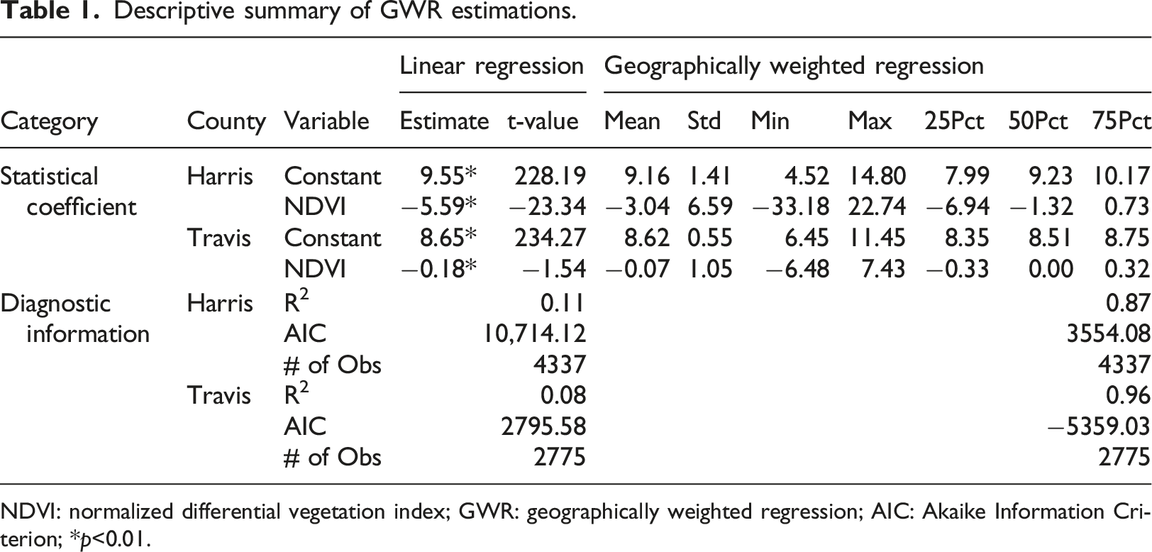
NDVI: normalized differential vegetation index; GWR: geographically weighted regression; AIC: Akaike Information Criterion; *p<0.01.
Figure 1 presents the outputs of downscaled PM2.5 concentrations in both Harris and Travis counties. Satellite-derived estimations of PM2.5 (unit: μg/m3).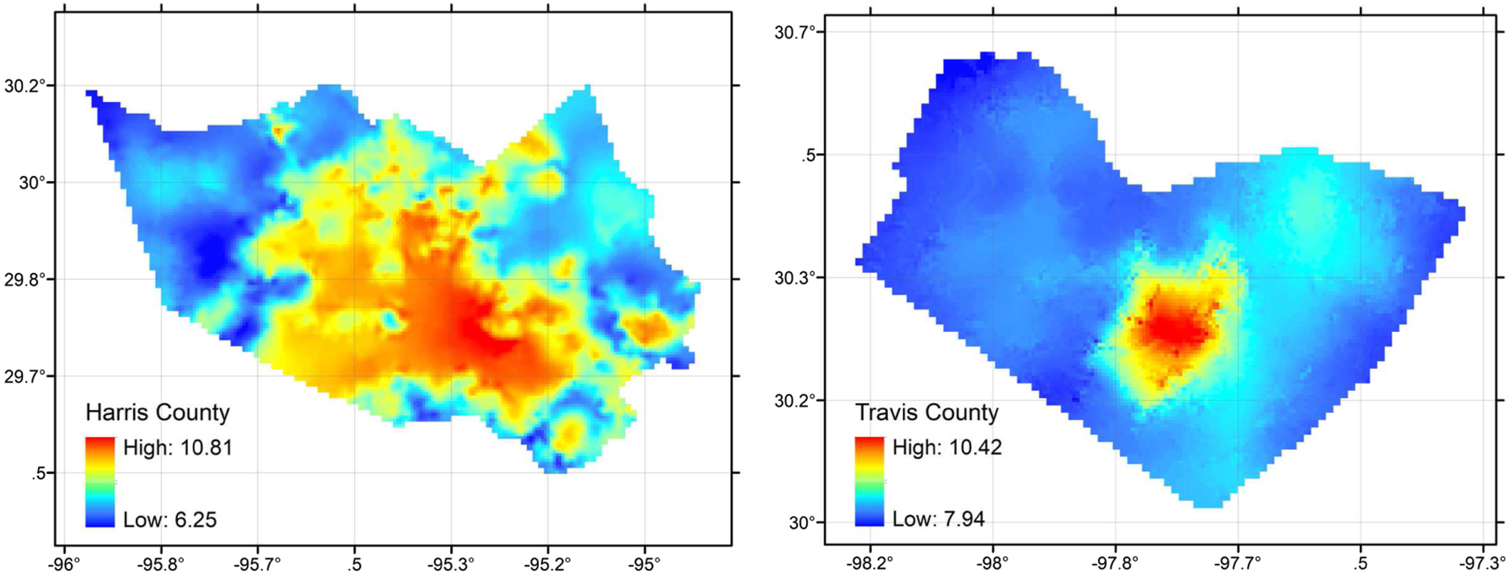
Urban metrics and database
We develop diverse urban metrics in the following four categories: urban structure, vehicle miles traveled (VMT), distance to road, and land use/land cover (LULC), in order to explore the spatial patterns of PM2.5 levels caused by heterogeneous urban metrics in three-dimensional space. We then implement grid tessellation to save all urban metrics as a data inventory for statistical analysis. Finally, we superimpose the urban metrics onto each cell.
Implementation of database
We integrate all urban metrics into regular grid tessellations over Harris and Travis counties for statistical modeling. The cell size is 0.05° by 0.05°, corresponding to the image resolution of PM2.5 concentration. This overlay process helps to create a unique database with diverse input resources at fine spatial scales. We determine a representative value for each variable within a cell, using the spatial analysis for distance from traffic roads, the percentage of each land classification within a cell for LULC, average values for all urban structures, the total length of lane miles, and a summation of all values for all VMT and total length of lane miles.
Urban structure
Under this category, we employ three key urban features—building mass, total length of lane miles, and tree canopy. We compute building mass by using building ground areas weighted to building heights within a given unit cell. To measure it, we employ a 3D model with the help of both a LiDAR dataset and GIS building footprints, and then superimpose the 3D model onto the grid tessellation. Within a given unit cell, we compute a representative value of building mass so that the impact of building density on PM2.5 can be appropriately explained. We estimate the total length of lane miles by summing up all traffic roads within a cell to reflect the effects of road network density. Finally, we use the percentage of tree canopy coverage provided by the Multi-Resolution Land Characteristics consortium to understand the impact of tree canopy on PM2.5 concentrations.
Distance to road
The gradient ratios of air pollution levels near the traffic networks are important to understanding and reducing the negative impact on health of air pollutants formed by vehicular emission. Texas Department of Transportation publishes annual roadway inventory data that include GIS linework and all roadway attributes. We use the 2017 roadway inventory annual data. Based on the functional classification in the attribute table, we create seven subsets, including interstate highways, freeways and expressways, principal arterials, minor arterials, major collectors, minor collectors, and local roads. Then, using the Near tool in ArcMap, we measure the distance from an individual cell to each road segment category.
Daily VMT
Travel by motorized vehicles is a key element for investigating air pollution near traffic networks. Using traffic volume as measured by TxDOT, we calculate three types of VMT based on the Federal Highway Administration (FHWA) vehicle classification—daily passenger car, light truck, and heavy truck VMTs. The FHWA classifies passenger cars with class numbers 1 through 4, light trucks (Single-Unit trucks) with class numbers 5–10, and heavy trucks (Combination trucks) with class numbers 11–13. This data allows us to understand the impact on PM2.5 concentrations of mobile emissions by specific types of traffic. For more detail on the FHWA classification, see Traffic Monitoring Guide (U.S. Department of Transportation, 2016). By superimposing the traffic network with VMT onto each cell, we obtain the total daily VMT per type of vehicle.
National land cover data
This study investigates the contribution to PM2.5 concentrations of LULC, which we measured using the National Land Cover Data (NLCD) from the U.S. Geological Survey. The NLCD, based on satellite images captured by Landsat TM, provides 15 LULC patterns with a spatial resolution of 30 m over both Harris and Travis counties. These data help to address some of the limitations of traditional GIS land-use data pertaining to uniformly developed information, data size, and incomplete information. In this study, we employ the 2016 dataset to match the point, while satellite sensors measure PM2.5 information.
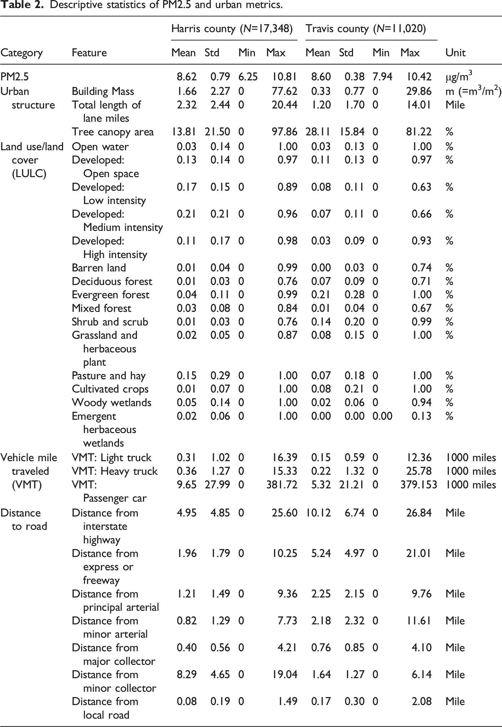
Descriptive analysis
Descriptive statistics of PM2.5 and urban metrics.
Method for data analysis
This study uses a ML technique to assess the impacts of urban metrics on PM2.5 concentrations. By using the RF method, we extract key feature variables from each urban metric category. Random forest is composed of a large number of decision trees, which create a supervised classification approach called ensemble learning technique. Its element, the decision tree, consists of a sequence of nodes hierarchically connected by branches to repeatedly find an optimal solution for the decision at each step until nothing can be gained from extending the tree further. With this concept, the RF algorithm finds the best solution with high accuracy by averaging the results of numerous decision trees and reducing the variance. Random forest regression uses the weighed mean squared error (MSE) to split the training dataset for each decision tree algorithm. With an out-of-bag estimator, an algorithm for measuring the prediction error, RF calculates the MSE to categorize into feature i at a specific node, which is formulated for a given node by equation (1). Then, each tree picks a value with the smallest MSE to minimize residuals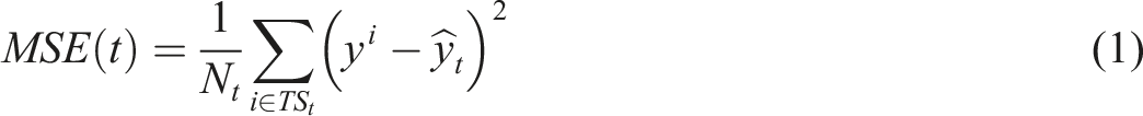
To measure each urban metric’s contribution to the PM2.5 concentration, we employ the Shapley value of the Gini impurity based on game theory, revealing unveiled information to explain the impacts of urban metrics on PM2.5 concentration by the RF models (Aldrich, 2020). This study used the Shapley value to estimate the marginal contribution of each variable in a model. The Shapley value, originating from cooperative game theory, is estimated by an imputation based on the combination of the power of each of the variables in equation (2) and the probability of joining possible coalitions in equation (3), which is a weight value to calibrate the power of variables

Results
This section presents results from three approaches: global Shapley value analysis, local Shapley values analysis, and greening scenario for PM2.5 removal.
Global Shapley value analysis
For RF modeling, this study randomly extracts 90% of all samples in each county (Harris County = 15,613; Travis County = 9918) as training sets and classified these datasets to avoid using them for the accuracy test of RF models. Figure S3 in Supplementary Materials presents MSE variations in training and testing data to determine optimal model parameters, especially the number of decision trees and their tree depths. First, more ensembled decision trees made the RF model stable for MSE. This study develops RF models under the assumption that the optimal decision tree number is 20 to avoid unexpected overfitting according to MSE variations. In addition, we use decision trees having depths less than 20 to run the RF model efficiently. The accuracies of the final RF results for Harris County and Travis County were R2 = 0.90 and R2 = 0.85, respectively.
Figure 2 summarizes the important features developed by the Shapley value with the RF algorithm. The summary plot of the Shapley value for each feature consists of points transitioning from a blue color, representing less of a contribution to PM2.5 levels, to a red color, representing more of a contribution to PM2.5 levels. Furthermore, the features are listed from the most significant to the least significant variable. Developed land-use features were significant in predicting PM2.5 concentrations in Harris County. Specifically, the feature “Developed: Medium and High Intensity” had high positive SHAP values in the plots, indicating that their density contributed to enhancing PM2.5 concentrations. In other words, these land-use patterns may generate relatively large amounts of PM2.5 and contribute to stagnant air pollution because many adjacent high-rise buildings inhibit air ventilation effects, supporting the positive impacts of Developed: Medium and High Intensity features in the predictions. The SHAP values of building mass support the proposition that densely clustered buildings tend to increase PM2.5 levels. Conversely, Pasture and Hay leads to decreases in the levels of PM2.5, which is negatively correlated with Developed: Medium and High Intensity. In addition, Tree Canopy Area tends to have statistically significant and negative effects on PM2.5 levels. This means that greening space can effectively filter small air pollutant particles, reducing their dispersion. Several studies have investigated the effects of vegetation on the number of air pollutants (Janhäll, 2015; Wolch et al., 2014). As expected, most of the features under the distance category were negatively associated with PM2.5 concentrations. In the case of Travis County, the distance measures appear to be more important than any other predictors. This result is partly due to the urban footprint along the major road networks in the county. Unlike Harris County in which the urban footprint spreads out in all directions and several urban ring roads serve the area, the urbanized area in Travis County mainly stretches north and south, and the major roads (Texas 1 Loop, I-35, and US 183) run in the same direction. Most of the county’s land is undeveloped or remains as green space. As a result, we expected to observe higher levels of PM2.5 near these major roads, mostly located between longitudes −97.7° and −97.8°. See Figure 1. As with the model for Harris County, vegetation is significant in predicting PM2.5 concentrations in the Travis County model. Specifically, Grassland/Herbaceous and Evergreen Forest are negatively associated with PM2.5 levels, which implies that greening space can play an important role in the reduction of pollutants. Comprehensive feature importance plots. (a) Harris County and (b) Travis County.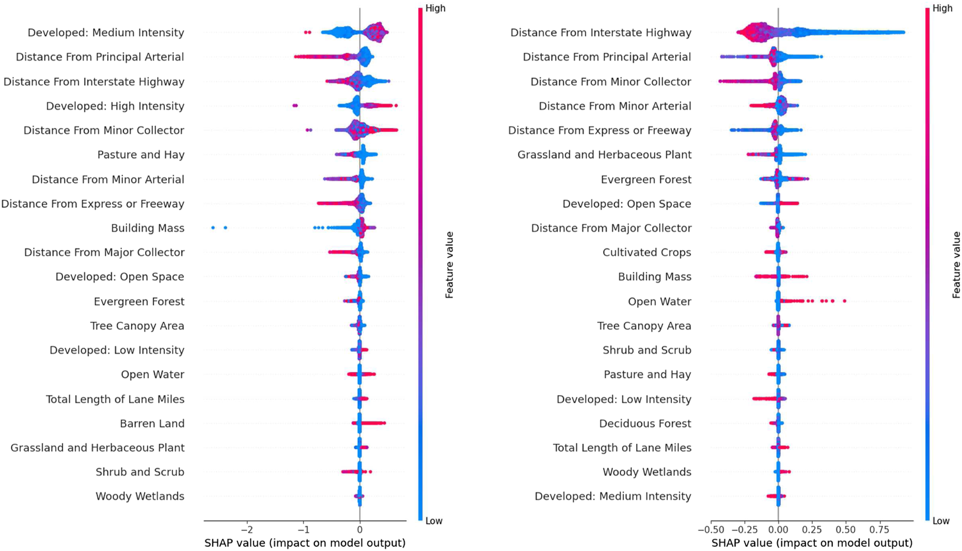
Interestingly, VMT features were not significant in predicting PM2.5 concentrations in the global Shapley value analysis in either Harris or Travis counties. However, the pollution levels around major traffic roads are relatively high so far. Thus, this study conducted further analysis of PM2.5 concentrations near major traffic networks, especially focusing on the areas containing interstate highways, expressways and freeways, and principal arterials.
Local Shapley value analysis
Given the results of the global SHAP analysis, we explore a more specific question: what types of urban features predominantly affect PM2.5 levels near major traffic networks? To address this question, we first extract only the cells with any of three primary traffic roads, including interstate highways, expressways and freeways, and principal arterials. The number of cells is 3544 out of 17,384 cells in Harris County, and 1245 out of 11,020 cells in Travis County. They account for approximately 20.4% and 11.3% of all cells in each county. Second, we identify existing land-use patterns to understand the settings of human activities. Third, we estimated additional SHAP values using urban structure and VMT with statistical simulation based upon scenario analysis to develop a physical urban design strategy for decreasing PM2.5 levels at a local scale.
Figure S4 in the Supplementary Materials describes LULC patterns near major traffic networks. As expected, developed LULC features were dominantly placed in both Harris and Travis counties. These patterns exist to afford better accessibility to residential places, commercial districts, and diverse pieces of infrastructure. Interestingly, the proportion of greening-related LULC patterns in Travis County is considerably higher than in Harris County. This result is due in part to the presence of more green spaces along the major roads in Travis County. Employing a greenbelt strategy to prevent urban sprawl, planners in Travis County have designed traffic roads to avoid any destruction of the existing greening space.
Figure 3 provides the SHAP values near major traffic networks. It indicates that building mass and total length of lane miles predominantly affect PM2.5 concentrations, with an R2 of 0.51 in Harris County and an R2 of 0.48 in Travis County. Based on these results, the building mass feature explains high levels of PM2.5 that can be triggered by numerous tall buildings, which generate stagnant air pollutants at the ground level due to poor ventilation effects. Previous studies have found that the phenomenon, the so-called street canyon effect, tends to enhance urban heat island intensity as well as air pollutant concentration (Fu et al., 2017). Feature importance plots for areas near major traffic networks. (a) Harris County and (b) Travis County.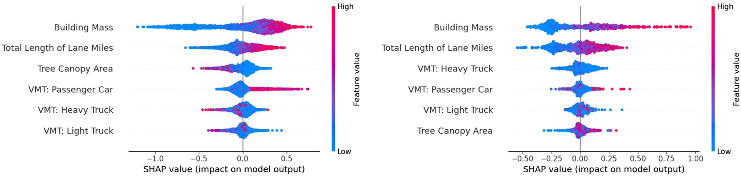
The total length of lane miles is also positively associated with PM2.5 concentrations. It indicates more total length of lane miles within a given unit area reflects an increase in the number of vehicles traveling, with corresponding high emission rates. Table S1 in the Supplementary Materials shows the distributed patterns of lengths of lane miles and VMT categorized by functional classification. Lengths of lane miles in the three main functional classes occupy about 12.7% of areas in Harris County and 11.9% of areas in Travis County, relatively small portions, while more than 40% of each of these three VMTs was measured by these classifications. It is undeniable that interstates, express/freeways, and principal arterials potentially generate substantial amounts of PM2.5, from volatile organic compounds in traffic emissions to brake and tire wear emissions.
Scenario analysis for PM2.5 removal: Building mass reduction and tree canopy expansion
From a planning perspective, there is no doubt that authorities should seek to alleviate the potential risks of PM2.5 exposure to achieve sustainable and healthy environments. The results of the RF analysis lead to the key question, “So now what?” What types of urban features can help reduce PM2.5 levels? How much do we need to utilize urban features? To address these questions, we use the outputs of local SHAP analysis in scenario analyses of building mass and tree canopy. As building mass is the most important feature in the output of local SHAP analysis, the impact of its reduction on PM2.5 needs to be demonstrated. In addition, although the effect of tree canopy area on the PM2.5 level is relatively weaker than those of other features, the strategy of addressing PM2.5 levels by increasing tree canopy cover is cost-effective, especially compared to alteration of building mass, total lane mileage, or traffic flows. Hirabayashi (2021) demonstrates the efficacy of urban forests in air pollutant removal, especially during hot seasons when removal peaks due to the enhanced pollutant filtering capability of urban vegetation.
We consider 0–50% decreases in existing building mass and 0–50% increases in tree canopy area in each 0.05° × 0.05° cell. We assumed that the maximum potential green space is 50% of the existing tree canopy area within a unit cell, counting parking and vacant lots as well as pedestrian streets as potential new green spaces.
Figure 4 visualizes the outputs of both building mass and tree canopy simulations. The red and green lines represent the variation in averaged PM2.5 concentrations as affected by 0–50% decremental and incremental changes in the variables in Harris and Travis counties. The lines indicate that a certain amount of each variable is required for effective PM2.5 mitigation. Each potential variation in PM2.5 levels by building mass and tree canopy simulations (unit: μg/m3).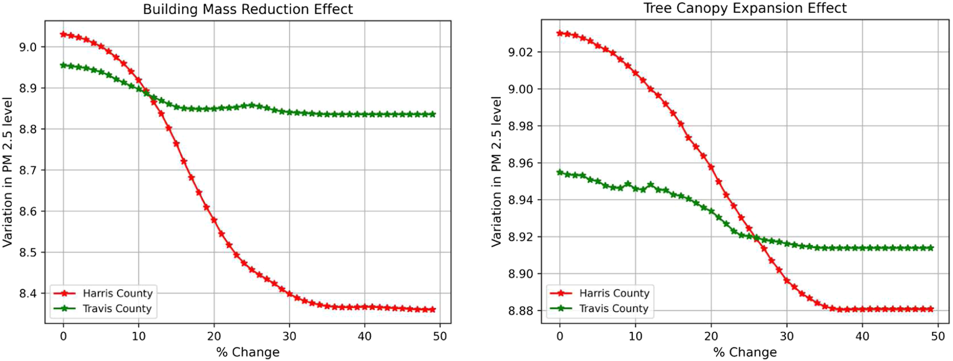
First, the reduction in building mass in Harris County had a positive effect by decreasing PM2.5. A minimum 10% decrease in building mass leads to a 0.1 μg/m3 reduction in PM2.5. However, this analysis showed that Travis County cannot achieve a dramatic reduction, based on the average PM2.5 concentrations in 2017. This scenario for Travis County may be closely associated with the existing spatial pattern of building mass. Relatively tall buildings are densely placed along I-35 Expressway, implying that the density pattern is based on a flat gradient. Thus, we predict that the effect of building mass reduction in Travis County is not significant because building mass in peripheral urban areas is less than in the central business district.
Second, In the case of Harris County, an increase in tree canopy area of at least 10% can reduce levels at most 0.02 μg/m3. With more than 10% in additional tree canopy areas, PM2.5 concentrations drop more rapidly, yielding more effective results. Interestingly, at increases of 35% or more, the tree canopy areas do not have any further effect on PM2.5 concentrations. In Travis County, under the assumption that there are available lands, a 25% increase in tree canopy areas reduces PM2.5 concentrations by only 0.03 μg/m3. Compared to the impact in Harris County, the maximum reduction effect of 0.03 μg/m3 predicted by the scenario analysis for Travis County is relatively small. The difference may pertain to the existing amount of greening space. Because of the presence of a large amount of greening space in Travis County, additional plants contribute less to reducing PM2.5 concentrations. Conversely, despite the need for relatively more green space, Houston, which has no land-use regulations, is very dense with more impervious areas spreading out. However, this analysis shows that an amelioration of the infamous zoning strategy in Harris County has great potential for improving air quality. The output of scenario analysis supports the efficacy of additional greenery along the major traffic networks in Harris County.
Conclusion
This study has examined the relationships between PM2.5 levels and urban features by employing an RF modeling technique for Harris County and Travis County in Texas. We used a GWR downscaling method for estimating PM2.5 levels. We also used Shapley values to understand the outputs of RF as well. Our findings emphasize that developed land use, tall buildings in dense areas, and areas adjacent to major traffic networks are the key drivers of PM2.5 concentrations. It is important to reduce the concentrations of PM2.5 by focusing on urban areas near major traffic roads. We have demonstrated the effects of tree canopy coverage to reduce PM2.5 levels through a greening scenario analysis. It is difficult to predict future PM2.5 levels accurately from tree canopy coverage alone because complex urban features continuously produce unexpected interactions. However, this type of approach helps to highlight the importance of greening space for improving air quality. It suggests the need for a planning framework for what local areas need to do and how they should handle their environments.
Although the research methodology for this study is new, it raises some questions for further research. First, this study employed PM2.5 images derived from MODIS satellites with 1 km spatial resolution. However, such spatial resolution is too coarse to identify the impact of each urban feature and to develop urban design strategies in detail. This study addressed the issue of resolution with GWR modeling with NDVI. This approach raises a GWR modeling question. Is the use of NDVI only the best option? In this study, R2 values of 0.87 in Harris County and 0.96 in Travis County were high enough to be statistically acceptable, but obviously, the result was affected only by the greenery pattern to determine PM2.5 levels. Second, the small impacts of VMT features on PM2.5 concentrations raise another research question. Intuitively, VMT features are likely to be an underlying source of air pollutants in urban settings. In this study, their importance was close to zero, implying that VMT had nearly no effect on PM2.5 levels. This may partly be due to the imbalance in traffic assignment on road segments. Usually, traffic volume counted at monitoring stations is assigned to any road segment, based on functional classification. However, this approach does not guarantee the traffic balance that occurs in the real world. For example, an origin–destination matrix in the travel demand model assumes that the total number of trips from origin i is equal to the total number of trips to destination i. Thus, this may be a cause of nonsignificant VMT effects. To overcome these drawbacks, further research, which includes more specific and realistic applications in planning practice, is required.
Supplemental Material
sj-pdf-1-epb-10.1177_23998083221078306 – Supplemental Material for Key determinants of particulate matter 2.5 concentrations in urban environments with scenario analysis
Supplemental Material, sj-pdf-1-epb-10.1177_23998083221078306 for Key determinants of particulate matter 2.5 concentrations in urban environments with scenario analysis by Bumseok Chun, Kwangyul Choi and Qisheng Pan in Environment and Planning B: Urban Analytics and City Science
Footnotes
Declaration of conflicting interests
The author(s) declared no potential conflicts of interest with respect to the research, authorship, and/or publication of this article.
Funding
The author(s) disclosed receipt of the following financial support for the research, authorship, and/or publication of this article: This work was supported by U.S. Department of Transportation.
Supplemental material
Supplemental material for this article is available online.
References
Supplementary Material
Please find the following supplemental material available below.
For Open Access articles published under a Creative Commons License, all supplemental material carries the same license as the article it is associated with.
For non-Open Access articles published, all supplemental material carries a non-exclusive license, and permission requests for re-use of supplemental material or any part of supplemental material shall be sent directly to the copyright owner as specified in the copyright notice associated with the article.