Building energy consumption and urban form: A multi-temporal empirical investigation

Abstract

Buildings are a main contributor to global energy consumption, with urban form significantly affecting their energy use. To quantify these effects, many studies relied on simulated data for limited buildings or empirical data at coarse temporal scales (monthly or yearly). However, few studies conducted large-scale empirical analyses of hourly consumption. In this paper, we empirically evaluate the impacts of urban form on energy consumption across multiple temporal scales (hourly, daily, monthly, and daily peak) for residential and commercial buildings in Santa Clara, CA. Using population density as a proxy for urban form, we built regression models and analyzed non-linear relationships and interaction effects. Results show that energy use intensity (EUI) varies non-linearly and significantly with population density, building size, and building use type. By increasing population density by one level , hourly EUI could drop by up to 32%, 36%, and 74% for single-family residential, multi-family residential, and commercial buildings respectively. The trends and magnitudes are consistent across temporal scales for the same building use type and population density level. These findings can inform decision-making regarding land use and urban planning for decarbonization goals and demand-side management programs.

Keywords

building energy modeling density urban form

Introduction

Increasing global energy demand has become a pressing concern in recent decades. Buildings are responsible for 30% of global energy use and 28% of CO₂ emissions worldwide (IEA, 2019). As urbanization progresses, urban population is expected to grow from 56.2% in 2020 to 68.4% in 2050 (United Nations, 2018), leading to a significant increase in energy demand and greenhouse gas (GHG) emissions. In addition, buildings today are not using energy efficiently. For instance, 75% of the building stock in Europe is energy inefficient (European Commission, 2020). Given that many countries have set decarbonization goals, we need a deeper understanding of how people use energy in the urban environment, necessitating the use of Urban Building Energy Modeling (UBEM).

Drivers of building energy use include not only the building properties but also the urban form in which buildings are situated. Urban form, also known as urban morphology, refers to the spatial configuration of buildings and public spaces within a city. Urban form impacts building energy consumption by posing physical obstructions and altering the microclimate around buildings through solar radiation (Chatzipoulka et al., 2016; Cheng et al., 2006; Li et al., 2018; Shishegar, 2013; Strømann-Andersen and Sattrup, 2011; Van Esch et al., 2012), airflow patterns and wind speed (Chen et al., 2017; Deng et al., 2016), and other attributes (Ahmadian et al., 2021; Krüger et al., 2010; Wong et al., 2011).

Investigations into the impact of urban form on energy use date back to the last century. Researchers have studied various urban form variables including building type and size, compactness, building coverage ratio, floor area ratio, urban canyon height to width ratio, and vegetation coverage (Ahmadian et al., 2021; Ahn and Sohn, 2019; Asfour and Alshawaf, 2015; Chatzipoulka et al., 2016; Cheng et al., 2006; Deng et al., 2016; Doherty et al., 2009; Ewing and Rong, 2008; Ko and Radke, 2014; Krüger et al., 2010; Li et al., 2018; Ourghi et al., 2007; Pisello et al., 2012; Rodríguez-Álvarez, 2016; Salvati et al., 2019; Shishegar, 2013; Steemers, 2003; Strømann-Andersen and Sattrup, 2011; Tereci et al., 2013; Van Esch et al., 2012; Wong et al., 2011). Many more urban form variables are summarized in (Ko, 2013; Narimani Abar et al., 2023; Quan and Li, 2021; Silva et al., 2017). Since 2008, interest in this field has increased, with a rise in physics-based studies and a recent resurgence in data-driven studies (Quan and Li, 2021).

The two modeling approaches exhibit clear distinctions. Physics-based models simulate the heat transfer processes that occur within and around buildings, capturing the influence of the surrounding urban form. For example, (Krüger et al., 2010) evaluated the impact of street canyon geometries on simulated cooling load of a residential building in a hot, dry environment, finding that taller buildings and narrower streets can reduce cooling loads in arid regions. Additionally, (Strømann-Andersen and Sattrup, 2011) employed thermal and daylight simulations to analyze passive solar gains in various urban canyon scenarios. They discovered that the geometry of urban canyon could impact total energy consumption by up to 30% for offices and 19% for housing compared to unobstructed sites in northern Europe.

To quantify inter-building effects, (Pisello et al., 2012) used EnergyPlus to simulate energy performance of a network of twenty single-family homes compared to standalone buildings. Their findings showed that proximity effects can lead to modeling inaccuracy of up to 42% in summer and 22% in winter. Building on this, (Han et al., 2017) examined mutual shading and reflection, concluding that shading has a larger impact on energy consumption than reflection. Additionally, (Chen et al., 2017) investigated the impacts of building height variations and building densities on urban ventilation, using wind tunnel experiments and computational fluid dynamic (CFD) simulations. They found that building height variation enhances ventilation for taller buildings but may worsen breathability for lower buildings. These studies concentrate on physically simulating building energy performance while accounting for surrounding urban context and microclimate to improve energy demand predictions. While physics-based approaches are generally more accurate, they require detailed building information and can be computationally prohibitive for large-scale urban simulations.

On the other hand, a shift toward data-driven studies has been observed as more energy datasets become available. For instance, (Ko and Radke, 2014) developed a statistical model to predict summer cooling electricity use for Sacramento, CA., incorporating occupant behavior, property characteristics, demographics, and urban form. They concluded that urban forms have a statistically significant impact on summer cooling energy. To optimize energy efficiency, it is beneficial to increase density and green space, maximize east–west street orientation, regulate floor area ratios and lot coverage for solar access, and incentivize appropriate tree planting.

Additionally, (Li et al., 2018) built a multilevel spatial regression model to characterize the impact of neighborhood density on household electricity use in Ningbo, China, finding density positively associated with electricity consumption in summer but not winter, with effects varying by dwelling type. More recently, (Li et al., 2023) explored spatial variations in residential energy usage intensity in Chicago, finding that urban porosity and roughness length have consistent spillover effects on building electricity usage intensity, with these relationships varying seasonally. Furthermore, (Ahn and Sohn, 2019) examined the impact of three urban form variables—lot coverage ratio, number of stories, and variation in building heights—on the energy consumption of multi-family housings in Seattle. Their results indicated that while floor area ratio and number of stories are not statistically significant, the overall energy consumption decreases in neighborhoods with higher lot coverage ratio and smaller building height variation, effective only within close range. In general, data-driven models are proven useful in specific scenarios but tend to have poor generalizability when applied to other contexts, as the data available for each project or location differs significantly.

Existing research has extensively explored the relationship between urban form and building energy use across various building types, regions, and climates, measuring diverse aspects of energy consumption under different scenarios. However, due to this contextual diversity, findings often present conflicting trends with little consensus about the impact of certain urban form variables (Narimani Abar et al., 2023).

In addition, limited data availability often constrains the scope and granularity in large-scale UBEM studies (Keirstead et al., 2012). In terms of scope, the focus on different building types is uneven across literature (Quan and Li, 2021), with more studies concentrating on residential buildings (Ahn and Sohn, 2019; Asfour and Alshawaf, 2015; Ewing and Rong, 2008; Han et al., 2017; Ko and Radke, 2014; Krüger et al., 2010; Li et al., 2018, 2023; Strømann-Andersen and Sattrup, 2011; Tereci et al., 2013) than commercial or office buildings (Deng et al., 2016; Ourghi et al., 2007; Strømann-Andersen and Sattrup, 2011; Wong et al., 2011). Research that consistently studies various building types is relatively scarce. Moreover, studies with moderate spatial granularity (e.g., building or parcel level) typically have poor temporal granularity for energy data (e.g., yearly or monthly). These yearly or monthly energy consumption data are typically made available by city governments for benchmarking purposes. However, even for proprietary data, high granular temporal and spatial energy information are unlikely to be available simultaneously because of privacy concerns. Therefore, longitudinal studies that can consistently track these effects across scales are desired.

Restricted by limited data availability and computational complexity, spatial modeling with rich urban context for large-scale energy analysis is challenging. Population density, however, an easily accessible demographic attribute, is often used to study the impact of urban form on energy use (Doherty et al., 2009; Ko, 2013; Ko and Radke, 2014; Narimani Abar et al., 2023; Quan and Li, 2021; Silva et al., 2017; Steemers, 2003). Compared to spatial characteristics required by many studies, population density can represent the aggregated effect of urban form, because it inherently captures information about the local planning regulations. While it provides a comprehensive picture of how people use energy across different urban forms, the effects of population density on building energy are complex and not fully understood (Silva et al., 2017).

In this paper, we empirically evaluate the impact of population density on building energy use using a large-scale dataset with hourly energy consumption data for residential and commercial buildings in Santa Clara, CA. We quantify the linear and non-linear effects of the variables on hourly, daily, monthly, and daily peak building energy use intensity. We examine whether high density may lead to non-linear increases in energy use while controlling for other building properties. We also examine if interaction effects exist between building size and population density. We discuss the results and implications of the models and explore how zoning policies can be beneficial for reducing building energy consumption in urban environments.

Methodology

Data collection

We obtained an energy dataset from Silicon Valley Clean Energy (SVCE) and combined it with publicly available tax assessor and census data to enrich the variable space. After cleaning and removing outliers, we used building energy use as the predicted variable and all other building properties as predictor variables. We employed separate datasets and models for various temporal resolutions (monthly, daily, hourly) and building use types (single-family residential, multi-family residential, commercial).

Energy consumption data

Our energy dataset contains hourly or 15-min energy consumption data from 170,224 SVCE customers in Santa Clara County, CA in 2018. The 15-min interval data was resampled to hourly (and subsequently daily and monthly) energy consumption for better generalizability.

Tax assessor data and census data

We retrieved tax assessor data from Santa Clara County and census data from the US Census Bureau and feature engineered predictor variables through simple calculations. Continuous variables include building floorspace, number of parcel units, year built, number of floors, building coverage ratio, land value, building value, and population density. For population density, we used residents per square mile for residential buildings and jobs per square mile for commercial buildings. Boolean variables indicate whether each building customer possesses one of the following: air conditioning, heating, battery electric vehicle (BEV), plug-in hybrid electric vehicle (PHEV), solar panels, and battery storage.

Weather data

To account for hourly building energy fluctuations due to weather, we obtained the 2018 local climatological data from the nearest weather station, San Jose International Airport, from (NOAA, 2018). We selected three key meteorological variables: hourly dry bulb temperature, relative humidity, and sky conditions as predictors. Sky conditions from the original dataset were presented as strings indicating up to three cloud layers, each characterized by one of 10 degrees of cloud obscurity (1 being clear, 10 being obscured). We converted these to float values by averaging the cloud layers. The average sky condition serves as a proxy for solar radiation received at buildings.

Complying with privacy regulations

Due to privacy regulations preventing raw energy consumption data at the building level being shared by SVCE, we grouped similar customers into clusters of 20 based on building properties. We then averaged the building properties and energy consumption across all customers in each cluster to obtain a reduced dataset. The detailed procedure is described in (Miotti and Jain, 2022). Although this clustering procedure inherently smoothens energy consumption spikes, each cluster’s average energy use still represents customers with similar building properties.

Feature engineering

After data cleaning, we divided energy consumption by building floorspace to calculate energy use intensity and applied logarithmic transformation to normalize it and handle skewness. Our predicted variable is therefore the log of energy use intensity.

In the monthly models, weather variables were not used as predictors. Besides the previously mentioned building properties from tax assessor and census data, we dummy encoded an additional predictor, month, into 12 indicator variables, allowing each month to have an independent effect on building energy use intensity. Therefore, the seasonal changes in weather are inherently captured in the month variables.

For the hourly models, we included three additional variables—season, hour, and weekday/weekend—as dummy variables to account for periodic energy use patterns. In addition, we added three weather variables: dry bulb temperature, relative humidity, and sky conditions, plus their averages from the previous 0–6, 6–12, 12–18, and 18–24 hours to capture their lagged effects. For the daily peak models, we used the weather variables at the peak hour and the corresponding averaged values in four intervals—12a.m.–6 a.m., 6a.m.–12p.m., 12p.m.–6p.m., and 6p.m.–12a.m.—of the previous day. Lastly, for daily models, we used the average weather values in these four intervals from both the previous and current day to capture the daily average weather.

After examining variable distributions, we applied logarithmic transformations to floorspace, land value, building value, and population density. As these variables were all right skewed and positive, the log transformation helped mitigate skewness and reduce the influence of extreme outliers, improving model stability and the interpretability of coefficients. We also found that models using log-transformed variables exhibited improved performance across different model variations.

Additionally, the range of population density was divided into eight levels: 0–500 persons per mi² (0–193 persons per km²), 500–1,000 persons per mi² (193–386 persons per km²), 1,000–2,500 persons per mi² (386–965 km²), 2,500–5,000 persons per mi² (965–1,931 persons per km²), 5,000–7,500 persons per mi² (1,931–2,896 persons per km²), 7,500–10,000 persons per mi² (2,896–3,861 persons per km²), 10,000–25,000 persons per mi² (3,861–9,653 persons per km²), and 25,000+ persons per mi² (9,653+ persons per km²). Table 1 shows example cities for all density levels. Satellite imagery of example census tracts in Santa Clara, CA, at each density level is provided in Table S1 in the supplemental material for direct comparison. Density was converted into dummy variables using one-hot encoding to capture non-linear relationships between density and energy use that cannot be adequately represented by a continuous variable or simple transformations. Similarly, the range of building floorspace was divided into seven levels: 0–1,000 ft² (0–93 m²), 1,000–2,000 ft² (93–186 m²), 2,000–5,000 ft² (186–465 m²), 5,000–10,000 ft² (465–929 m²), 10,000–20,000 ft² (929–1,858 m²), 20,000–50,000 ft² (1,858–4,645 m²), and 50,000+ ft²(4645+ m²), and floorspace was converted into dummy variables. We also included interaction effects between floorspace and density.

Table 1.

Example cities and census tracts for eight density levels.

Density level	Population density (persons per mi²)	Population density (persons per km²)	Example city/country	Example US city
0	0–500	0–193	Iceland	Anchorage, AK
1	500–1,000	193–386	Ulaanbaatar, Mongolia	Columbia, SC
2	1,000–2,500	386–965	Melbourne, Australia	Jacksonville, FL
3	2,500–5,000	965–1,931	Abu Dhabi, United Arab Emirates	Houston, TX
4	5,000–7,500	1,931–2,896	Istanbul, Turkey	San Jose, CA
5	7,500–10,000	2,896–3,861	Stuttgart, Germany	Los Angeles, CA
6	10,000–25,000	3,861–9,653	Singapore	San Francisco, CA
7	25,000+	9,653+	Paris, France	New York, NY

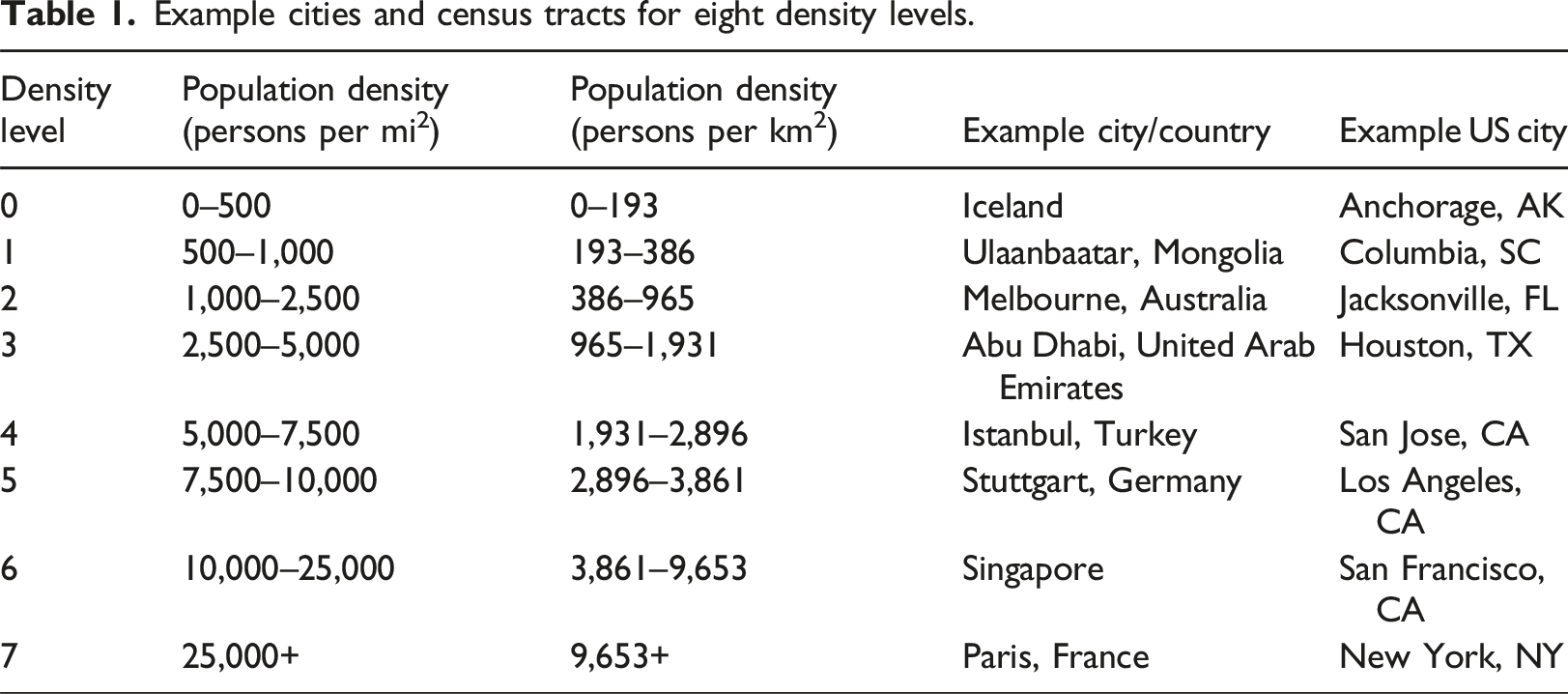
Modeling

To ensure consistency in our analysis, hourly data was resampled and fitted to daily and monthly models. For each temporal resolution, data from the three building use types were separated and fitted to different models respectively.

To study the relationship of interest in different scenarios, we defined two scopes for the hourly models.

• Scope 1 includes all 8,760 hours in 2018.

• Scope 2 is limited to 2p.m. to 6p.m. during demand response event dates in 2018 (nine summer weekdays), representing peak demand periods when the California power grid is under stress.

In addition to modeling energy consumption on a monthly, daily, and hourly basis, we also modeled daily peak energy demand. Consequently, we constructed 15 datasets total, covering five temporal scopes—monthly, daily, hourly scope 1, hourly scope 2, and daily peak—for each of the three building use types. For each dataset, we compared models with different feature selections (continuous vs dummy variables) based on the Root Mean Squared Error (RMSE) on a 30% testing set. A final model for each building use type and each temporal scope was selected and refitted using all the data and is presented in the following sections. Table S2 in the supplemental material summarizes the variables used for all 15 models. For residential buildings, we modeled floorspace as continuous and density as dummy variables, while for commercial buildings, both were modeled as dummy variables. This distinction also leads to the difference in interaction terms between floorspace and density: for residential models, they are continuous for each of the eight density levels, while for commercial models, they are all combinations of floorspace and density levels.

While more complex non-linear models could potentially capture additional patterns in the data, we chose linear regression for this study. Our model design already accounts for non-linearities through dummy variables and interaction terms, and the high R² values across our models suggest this approach successfully captures the key relationships. Given our goal of providing actionable insights, we prioritized model interpretability over additional model prowess.

We used the Python package Statsmodels (Perktold et al., 2023) to build linear regression models to quantify effects of variables on energy use intensity. We applied min-max scaling to bring all predictor variables to the same scale from 0 to 1. Using the predictors in Table S2, the predicted variable is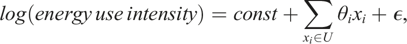

\log (e n e r g y u s e i n t e n s i t y) = c o n s t + \sum_{x_{i} \in U} θ_{i} x_{i} + ϵ,

where

θ_{i}

is the coefficient for variable

x_{i}

U

is the set of variables used in respective models, and

ϵ

is the error term.

Results and discussions

We explore the relationship between energy use and population density by examining the corresponding coefficients. Results for all 15 models are provided in the supplemental material (Tables S3–S7), including fitted coefficients, standard errors, and R² values. We will first discuss hourly models for single-family residential, multi-family residential, and commercial buildings, then compare these with other temporal scopes. Note that we only demonstrate results derived from significant coefficients, and not all curves cover the entire range of building floorspace. While no clear trend appears across density levels, consistent trends emerge across temporal scales for different density levels, which we will discuss in a later section.

Figure S1 in the supplemental material shows hourly scope 1 energy use intensity (EUI) for each density level relative to the reference point (density level 0 with smallest building size) for all three building types. Due to density-floorspace interactions, density effects on EUI depend on building size. In Figure S1(a) and S1(b), EUI decreases as building size increases for residential buildings, consistent with previous findings that larger homes are less utilized per unit area (Ahn and Sohn, 2019; Kontokosta, 2012; Kontokosta and Tull, 2017). This may be due to lower surface-to-volume ratios reducing heat transfer (Pacheco et al., 2012; Ratti et al., 2005; Sanaieian et al., 2014) and more advanced energy-saving technologies (Li et al., 2014) in larger buildings. For commercial buildings (Figure S1(c)), where both density and floorspace are modeled as dummy variables, EUI fluctuates with building size across density levels. Our analysis reveals that optimal density for minimizing EUI varies with building size across all models.

To better understand the impact of density on energy per square foot, we analyze percentage differences in EUI between consecutive density levels. This stepwise comparison offers meaningful insights for urban planning and policy-making, reflecting a practical progression for densification of a neighborhood or region.

Hourly models for single-family residential buildings

As shown in Figure 1(a), small single-family homes in density level 1 areas consume 27% less energy per square foot than those in density level 0 (blue curve), with a similar 32% reduction observed when comparing density level 7 to 6 (pink curve). For the least and most populated areas, slight densification is associated with a non-trivial amount of energy reduction, which diminishes as building size increases. Moreover, buildings in density level 3 consume about 5% less energy than those in level 2, regardless of building size (green curve). However, moving from density level 1 to 2 (orange curve) increases hourly EUI by about 2% for all building sizes, suggesting that single-family homes in density level 2 areas are relatively energy inefficient compared to neighboring density levels 1 and 3. This demonstrates that the effects of densification are non-linear and must be evaluated case by case.

Figure 1.

Hourly EUI reduction per density level increase for single-family residential buildings for (a) scope 1 (all hours in 2018) and (b) scope 2 (2p.m.–6p.m. during demand response event dates in 2018).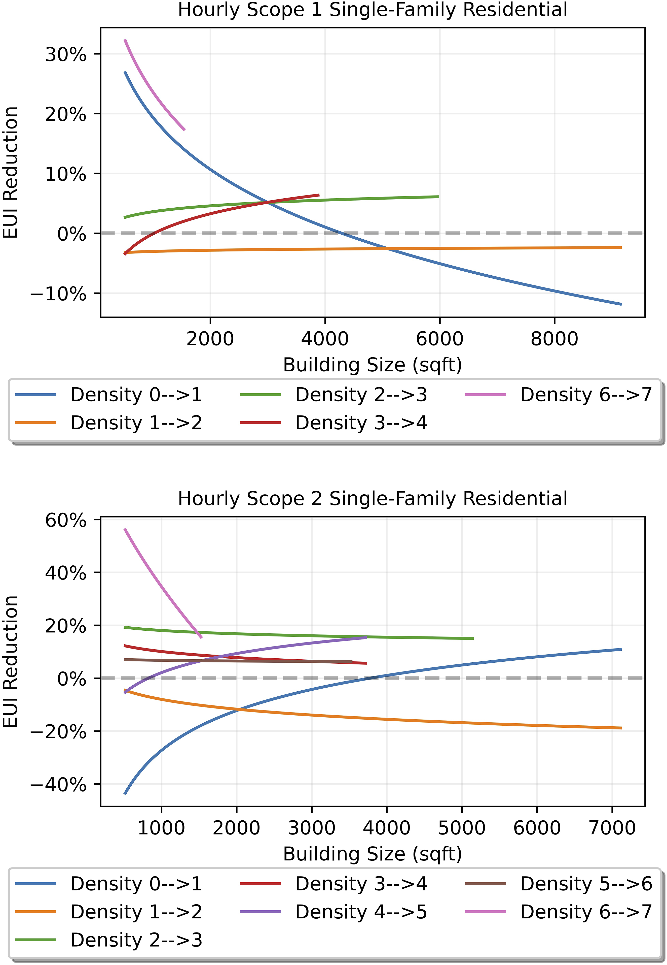

Unlike scope 1, which studies the general relationship across all 8760 hours, the hourly scope 2 model quantifies the effect of density on hourly EUI during demand response events in 2018. For single-family homes, energy savings increase with building size when comparing density levels 0 and 1 (blue curve in Figure 1(b)), contrasting with the trend in scope 1. This reversal likely stems from different energy use patterns in low-density areas during extreme weather compared to normal days. Moreover, buildings with floorspace between 1000 and 3500 ft² (93–325 m²) in the highest density level 7 are the most energy efficient, with progressive EUI reductions from density level 2 to 3, 3 to 4, 4 to 5, 5 to 6, and 6 to 7 during the hottest hours when the grid is likely overloaded. And the energy savings potential is notably higher than in scope 1, with up to 56% reduction when moving from density level 6 to 7. This is consistent with previous works that demonstrate that denser urban forms can lower EUI, especially in summer months, through increased shading, thermal mass, and higher efficiency of building energy systems (Ko and Radke, 2014; Strømann-Andersen and Sattrup, 2011). The hourly scope 2 multi-family residential and commercial models are not presented because there are too few data points in the multi-family dataset, and the commercial results are very similar to the scope 1 case.

Hourly model for multi-family residential buildings

Figure 2 illustrates that multi-family buildings in density level 2 areas consume significantly more energy per square foot compared to those in level 1 (orange curve), a pattern more pronounced than in single-family homes (orange curves in Figure 1(a) and (b)). In contrast, buildings in other density levels exhibit progressively lower EUI when compared to the previous density level, with reductions of up to 36%, 30%, and 20% for density levels 1, 3, and 4, respectively. These results reveal stark differences in energy use across multi-family communities in varying density regions. Except for density level 2 (orange curve), the findings generally align with previous studies, indicating that densification improves residential energy efficiency due to reduced heating energy (Rode et al., 2014) and the coupled effect of small housing (Ewing and Rong, 2008). Multi-family communities may benefit more from densification due to economies of scale and efficient use of district energy and shared resources (Brown and Logan, 2008; Hui, 2001; Resch et al., 2016).

Figure 2.

Hourly (scope 1) EUI reduction per density level increase for multi-family residential buildings.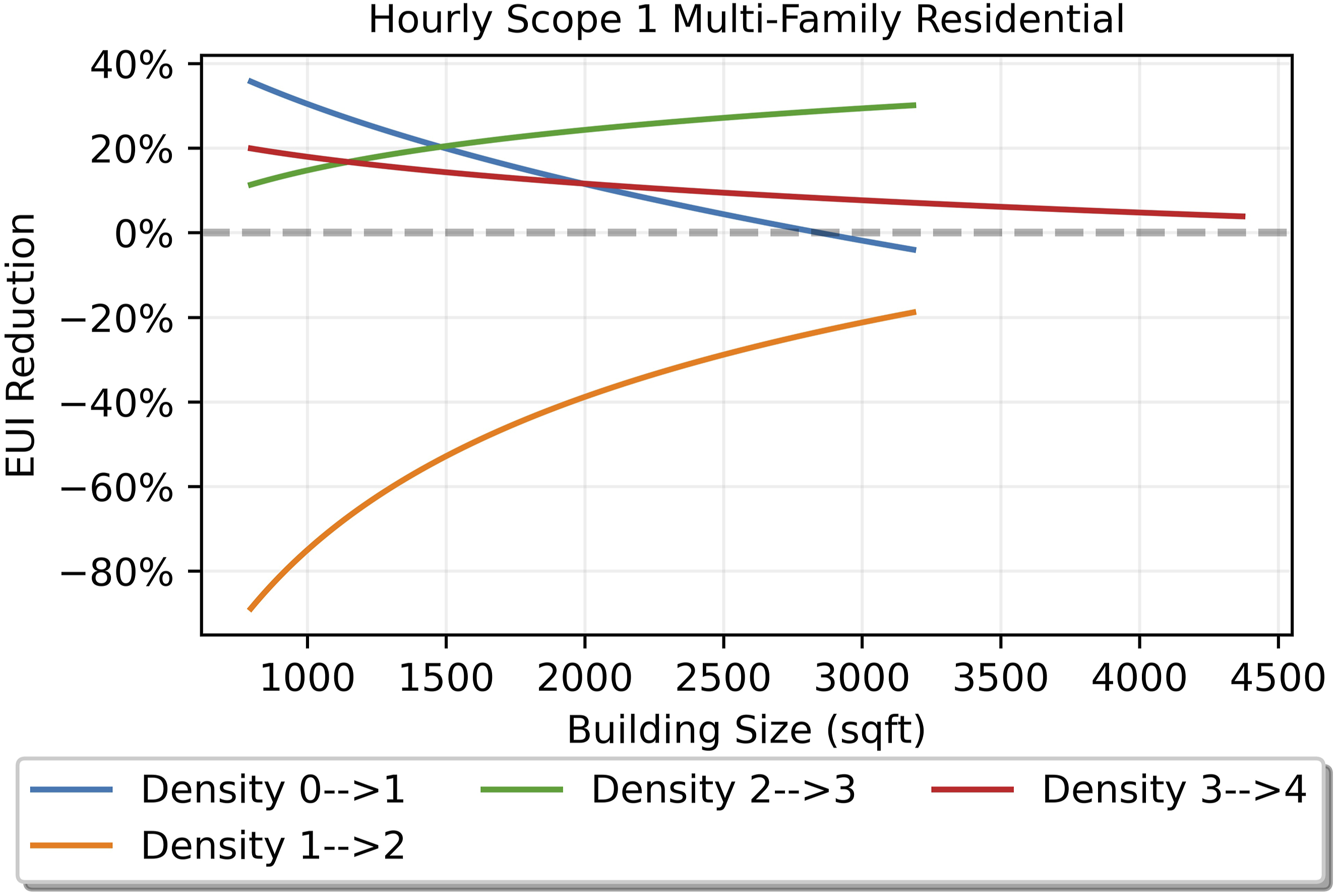

Hourly model for commercial buildings

For commercial buildings, energy consumption variations between density levels depend significantly on both density and building size. As shown in Figure 3, small commercial buildings (floorspace levels 0, 2, 3), when moving from density level 1 to 2 (in orange), exhibit up to 74% EUI reduction, contrasting with residential patterns in Figures 1(a) and (b), and 2. Another key difference emerges when increasing density from level 2 to 3 (in green): while residential buildings of all sizes show reduced energy use, only the largest commercial buildings achieve an energy reduction of 43%. Furthermore, small commercial buildings (size levels 1 and 2) in mid-density levels 3, 4, and 5 can achieve energy savings of up to 50% when moving up by just one density level.

Figure 3.

Hourly (scope 1) EUI reduction per density level increase for commercial buildings.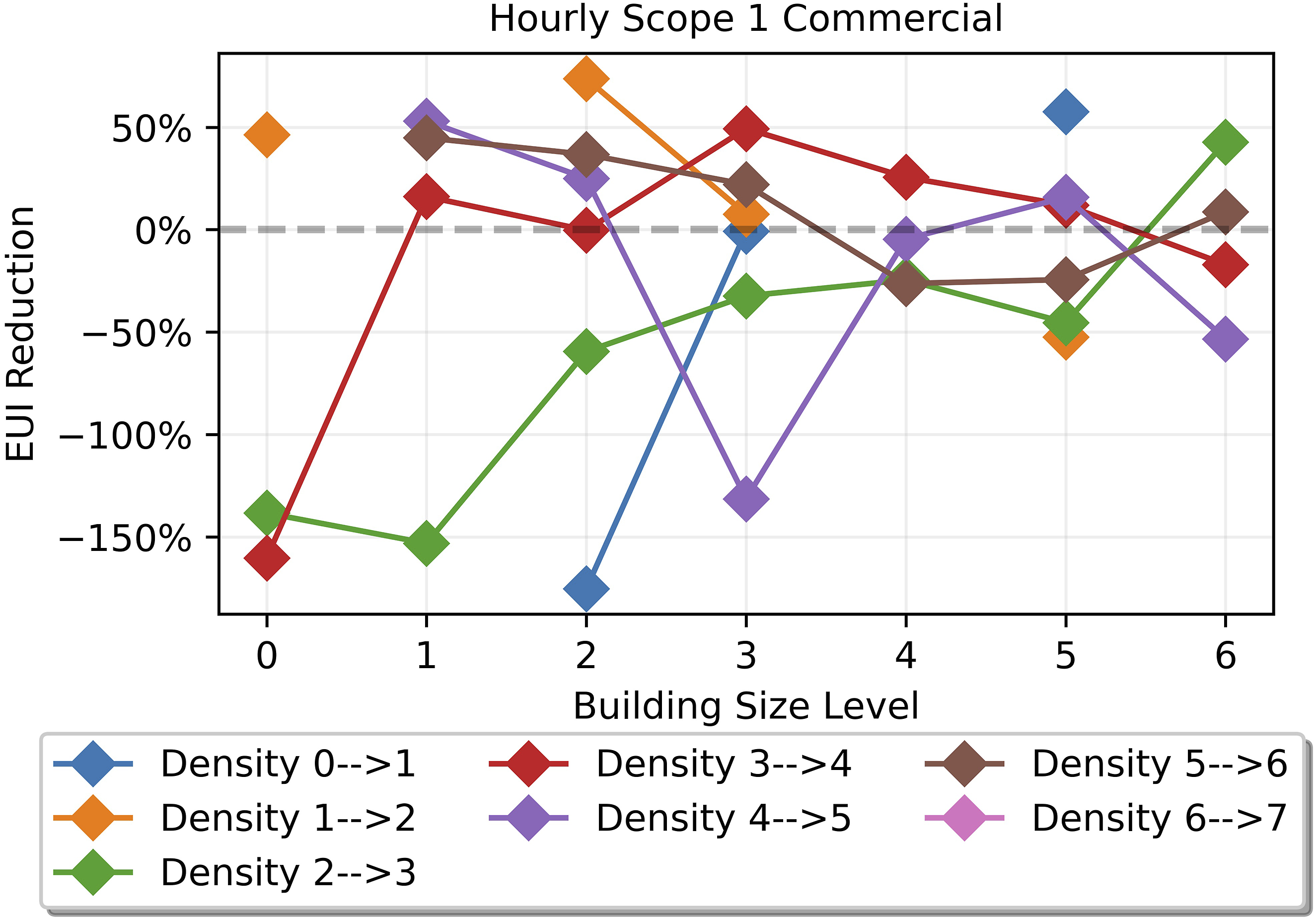

The inconsistent energy savings observed across different density levels and building sizes among all building types—single-family residential, multi-family residential, and commercial— reflect a complex relationship between urban density and energy consumption. While the conventional belief suggests that densification generally leads to lower energy use, numerous studies have reported conflicting findings, with some showing negative correlations, others positive, and some indicating that density is insignificant (Narimani Abar et al., 2023; Quan and Li, 2021). This complexity stems from multiple competing mechanisms: denser urban forms can reduce heating energy through shared walls and reduced exposure to cold winds, but may increase cooling and lighting energy due to urban heat island effects and reduced natural light penetration. Additional factors such as building characteristics, occupant behaviors, energy infrastructure, and climate further complicate this relationship, making the net effect highly context dependent. This study highlights the necessity of detailed analysis within specific contexts to accurately determine the impact of density on building energy consumption.

Daily, monthly, and daily peak models for single-family residential, multi-family residential and commercial buildings

The same analysis was conducted for daily, monthly, and daily peak models across all building types. Figure 4 presents the EUI reduction patterns for single-family residential models, while comparisons for the other two building types are provided in the supplemental material (Figures S2–S3). The trends of EUI reduction derived from the daily, monthly, and daily peak models are mostly consistent with the hourly models, with only minor differences. For example, large single-family homes exhibit a daily peak EUI reduction of up to 4% when moving from density level 1 to 2 (orange curve in Figure 4(c)), in contrast to a negative energy reduction for all building sizes in models of other temporal scales.

Figure 4.

EUI reduction per density level increase for single-family residential buildings on a (a) daily, (b) monthly, and (c) daily peak basis.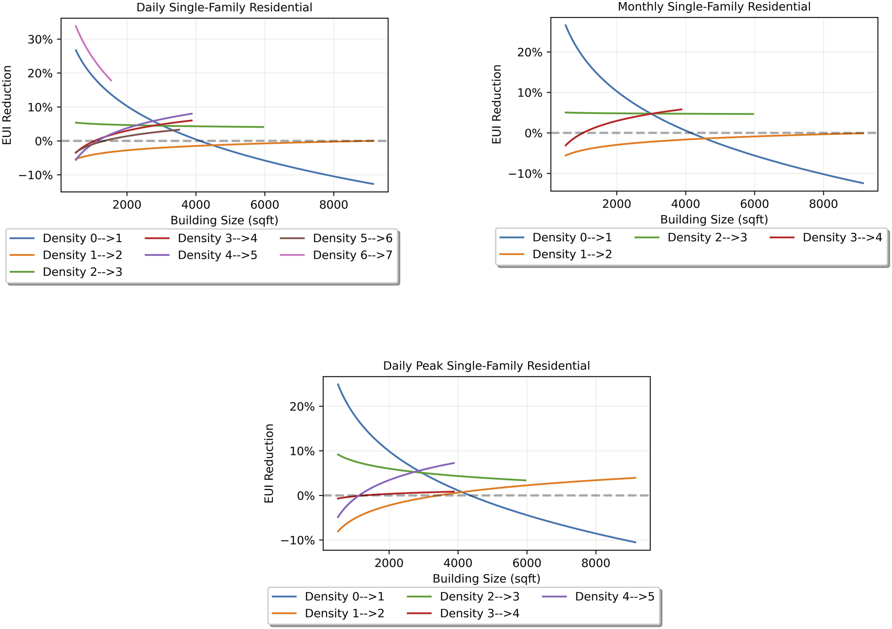

From the above results, the effects of density on building EUI vary across different density levels. In some cases, higher density results in lower EUI, aligning with the general rationale for densification (Ko and Radke, 2014; Strømann-Andersen and Sattrup, 2011). However, this does not apply to several corner cases, as shown in our analysis. In addition, the results are presented in terms of energy per square foot, indicating that the energy savings per capita may be even more significant when accounting for population increase. These insights are crucial for policy development. While building occupants cannot directly influence local population density, and moving to higher density areas does not instantly change their building energy consumption, city planners and policymakers can leverage this information to develop regulations and urban planning strategies that enhance energy efficiency. Local regulators can implement targeted densification programs through incentives in appropriate census tracts. At optimal population density levels, even modest increases in population density can yield significant energy reductions. This is particularly relevant for post-COVID central business districts that are exploring diversification of their building stock to include conversions of commercial buildings to multi-family residential and provide mixed-use neighborhoods.

Uncertainties

Beyond examining the significant coefficients, we observed consistent trends in standard errors and R² values across models of different temporal scales. The standard errors of the coefficient estimates (shown in supplemental material) are generally smaller in more granular models (hourly < daily < monthly), which suggests that the estimates are more precise at finer time scales. This increased precision is likely due to the larger number of data points available in the granular models. Conversely, R² values (shown in Table 2) are higher in more aggregated models (monthly > daily > hourly), indicating that these models capture a greater proportion of the variance in the data. This makes sense, as a larger amount of granular data often contains more noise, introducing a higher level of uncertainty and making it more difficult for the predictors to explain the variability.

Table 2.

Comparison of the R² values for all 15 models.

Model	Single-family residential	Multi-family residential	Commercial
Hourly scope 1	0.4207	0.8009	0.7368
Hourly scope 2	0.3684	0.8889	0.8741
Daily	0.5133	0.8690	0.7527
Monthly	0.6116	0.9018	0.7632
Daily peak	0.4525	0.8478	0.7777

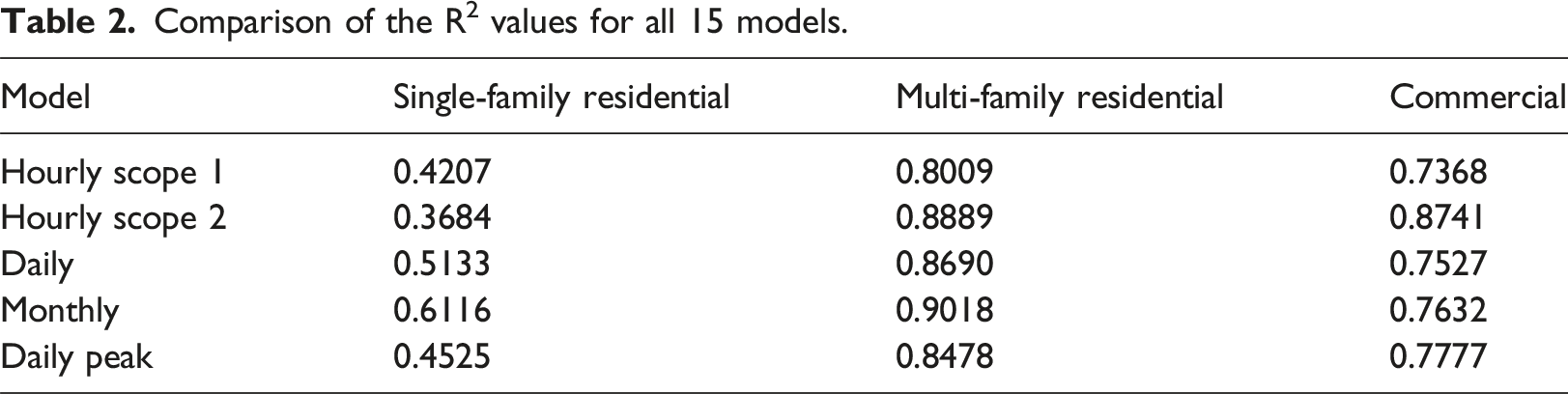
Similar trends are observed when comparing model results across building types. The significantly larger dataset for single-family residential buildings results in lower standard errors compared to multi-family residential and commercial models, reflecting reduced uncertainty in the estimates. On the other hand, the R² values for the single-family residential models are the lowest. This is likely because the large number of single-family homes may exhibit a wide variety of energy use patterns, making it challenging to capture this complexity with limited predictors. Notably, the R² values for all 15 models range from 0.3684 to 0.9018, which are generally higher than the values reported in existing studies (0.289–0.311 in (Ko and Radke, 2014) and 0.337–0.371 in (Ahn and Sohn, 2019)), highlighting the robustness of our approach in capturing the variance in energy use.

Limitations and future work

While our study provides valuable insights into the effects of population density as a proxy for urban form on building energy consumption, some limitations apply that could be addressed in future research. We represented urban form using only density. We believe this single-variable representation is appropriate because the scope of this study involves buildings in only one U.S. County (Santa Clara, CA), where the design and planning regulations can be assumed to be relatively consistent. Nonetheless, there might still be discrepancies in urban form among buildings with the same level of population density. Further analysis can help identify the factors contributing to lower energy usage in specific urban forms in Santa Clara. Additionally, clustering and averaging the original building properties to obtain typical building profiles was necessary for privacy compliance. Yet, even when the effects of the contributing factors may be averaged out, the model results were proven to be significant. Future research could explore the effects of other spatial features and interaction effects to facilitate a more detailed understanding. Lastly, we opted to use a simple statistical method, linear regression, to obtain easily interpretable results. While this method has proven useful, more complex models could provide more accurate quantifications of the effects of urban form while balancing accuracy and interpretability.

Conclusions and implications

This study empirically evaluated the impact of population density on building energy use intensity for single-family, multi-family residential and commercial buildings in Santa Clara, CA. By combining large-scale granular energy data with publicly available tax assessor and census data, we quantified the effect of density using linear regression models across temporal scales. The key contributions of this work include:

(1) We find empirical evidence that population density significantly impacts building energy use intensity. Increasing density solely while keeping all other variables constant could result in a reduction in hourly EUI of up to 32%, 36% and 74% for single-family, multi-family residential, and commercial buildings, respectively.

(2) We find that the impact of density is consistent across hourly (scope 1 and 2), daily, monthly, and daily peak energy use. This indicates that density changes could also play a role in temporal dependent energy usage and demand-side management.

These findings have important implications for urban planning, energy policy, and climate strategies. Specifically, this work supports the use of densification and mixed-use zoning as a tool to drive reductions in energy usage and realize additional benefits. It demonstrates the potential of using rich urban data to inform land use and density regulations. By understanding the nuanced effects of population density and urban form on building energy use, urban planners and policymakers can develop targeted strategies that optimize energy efficiency, achieve decarbonization goals, and support sustainable urban development.

Supplemental Material

Supplemental Material - Building energy consumption and urban form: A multi-temporal empirical investigation

Supplemental Material for Building energy consumption and urban form: A multi-temporal empirical investigation by Chi On Ho, Marco Miotti, and Rishee K. Jain in Environment and Planning B: Urban Analytics and City Science

Footnotes

Acknowledgments

We would like to thank Silicon Valley Clean Energy (SVCE) for their assistance in curating and providing the data utilized in this study.

ORCID iDs

Chi On Ho

Rishee K. Jain

Author Contributions

Chi On Ho: Conceptualization, Data Analysis, Writing—original draft. Marco Miotti: Data Collection, Writing—review & editing. Rishee K. Jain: Supervision, Writing—review & editing.

Funding

The authors disclosed receipt of the following financial support for the research, authorship, and/or publication of this article: The authors disclosed receipt of the following financial support for the research, authorship, and/or publication of this article: This work was supported by the National Science Foundation (NSF) [No. 1941695]; the UPS Endowment; and the Center for Integrated Facility Engineering (CIFE).

Declaration of Conflicting Interests

The authors declared no potential conflicts of interest with respect to the research, authorship, and/or publication of this article.

Data Availability Statement

The data that support the findings of this study may be available from the corresponding author upon reasonable request. Access to the data is restricted due to privacy, ethical, or legal concerns.*

Supplemental Material

Supplemental material for this article is available online.

Author biographies

Chi On Ho is a PhD candidate in Civil and Environmental Engineering at Stanford University, where she also earned her Master of Science degree. Her research lies at the intersection of urban analytics, building energy modeling, and simulation-based optimization, with a focus on data-driven approaches to sustainable urban systems. Prior to Stanford, she was a researcher at Engie Lab China and Disney Research China, contributing to projects ranging from district energy planning to computational design optimization. She holds a Bachelor’s degree in Civil Engineering from Tongji University and has published in both engineering and urban planning venues.

Marco Miotti is a Senior Researcher in the Ecological Systems Design group at ETH Zurich. His work focuses on investigating how urban form, human behavior, and technology interact in forming energy consumption and pollution patterns of cities, and how these interactions can be leveraged to reduce the environmental footprint of human activity.

Rishee K Jain is an Associate Professor of Civil & Environmental Engineering and a Chambers Faculty Fellow in the School of Engineering at Stanford University. His research interests lie at the intersection of data science, human dynamics and sustainable urban infrastructure systems. Rishee is a recipient of a CAREER Award from the U.S. National Science Foundation and a Building Innovator Fellowship from the U.S. Department of Energy.

References

Ahmadian

Sodagar

Bingham

, et al. (2021) Effect of urban built form and density on building energy performance in temperate climates. Energy and Buildings 236: 110762.

Ahn

Sohn

D-W

(2019) The effect of neighbourhood-level urban form on residential building energy use: a GIS-based model using building energy benchmarking data in Seattle. Energy and Buildings 196: 124–133.

Asfour

Alshawaf

(2015) Effect of housing density on energy efficiency of buildings located in hot climates. Energy and Buildings 91: 131–138.

Brown

Logan

(2008) The Residential Energy and Carbon Footprints of the 100 Largest U.S. Metropolitan Areas. Atlanta, GA: School of Public Policy, Georgia Institute of Technology, 79.

Chatzipoulka

Compagnon

Nikolopoulou

(2016) Urban geometry and solar availability on façades and ground of real urban forms: using London as a case study. Solar Energy 138: 53–66.

Chen

Hang

Sandberg

, et al. (2017) The impacts of building height variations and building packing densities on flow adjustment and city breathability in idealized urban models. Building and Environment 118: 344–361.

Cheng

Steemers

Montavon

, et al. (2006) Urban Form, Density and Solar Potential. In: The 23rd Conference on Passive and Low Energy Architecture, 2006.

Deng

J-Y

Wong

Zheng

(2016) The study of the effects of building arrangement on microclimate and energy demand of CBD in nanjing, China. Procedia Engineering 169: 44–54.

Doherty

Nakanishi

Bai

, et al. (2009) Relationships between form, morphology, density and energy in urban environments. GEA Background Paper 28.

10.

European Commission (2020) In Focus: Energy Efficiency in Buildings. Brussels: European Commission. Available at: https://commission.europa.eu/news/focus-energy-efficiency-buildings-2020-02-17_en (accessed 21 March 2024).

11.

Ewing

Rong

(2008) The impact of urban form on U.S. residential energy use. Housing Policy Debate 19(1): 1–30.

12.

Han

Taylor

Pisello

(2017) Exploring mutual shading and mutual reflection inter-building effects on building energy performance. Applied Energy 185: 1556–1564.

13.

Hui

SCM

(2001) Low energy building design in high density urban cities. Renewable Energy 24(3): 627–640.

14.

IEA (2019) The Critical Role of Buildings. Paris: International Energy Agency. Available at: https://www.iea.org/reports/the-critical-role-of-buildings (accessed 12 May 2023).

15.

Keirstead

Jennings

Sivakumar

(2012) A review of urban energy system models: approaches, challenges and opportunities. Renewable and Sustainable Energy Reviews 16(6): 3847–3866.

16.

(2013) Urban form and residential energy use: a review of design principles and research findings. Journal of Planning Literature 28(4): 327–351.

17.

Radke

(2014) The effect of urban form and residential cooling energy use in Sacramento, California. Environment and Planning B: Planning and Design 41(4): 573–593.

18.

Kontokosta

(2012) Predicting Building Energy Efficiency Using New York City Benchmarking Data. In: Proceedings of theACEEE Summer Study on Energy Ef iciency in Buildings, 2012.

19.

Kontokosta

Tull

(2017) A data-driven predictive model of city-scale energy use in buildings. Applied Energy 197: 303–317.

20.

Krüger

Pearlmutter

Rasia

(2010) Evaluating the impact of canyon geometry and orientation on cooling loads in a high-mass building in a hot dry environment. Applied Energy 87(6): 2068–2078.

21.

Hong

Yan

(2014) An insight into actual energy use and its drivers in high-performance buildings. Applied Energy 131: 394–410.

22.

Song

Kaza

(2018) Urban form and household electricity consumption: a multilevel study. Energy and Buildings 158: 181–193.

23.

Song

Kaza

, et al. (2023) Explaining spatial variations in residential energy usage intensity in Chicago: the role of urban form and geomorphometry. Journal of Planning Education and Research 43(2): 317–331. SAGE Publications Inc.

24.

Miotti

Jain

(2022) A Computationally Efficient Algorithm to Enable Privacy Preserving Urban Energy Data Sharing under the “15/15” Rule. Energy Proceedings 28.

25.

Narimani Abar

Schulwitz

Faulstich

(2023) The impact of urban form and density on residential energy use: a systematic review. Sustainability 15(22): 15685. Multidisciplinary Digital Publishing Institute.

26.

NOAA (2018) Maps and Geospatial Products. Washington, DC: National Oceanic and Atmospheric Administration. Available at: https://www.ncei.noaa.gov/maps-and-geospatial-products (accessed 17 May 2023).

27.

Ourghi

Al-Anzi

Krarti

(2007) A simplified analysis method to predict the impact of shape on annual energy use for office buildings. Energy Conversion and Management 48(1): 300–305.

28.

Pacheco

Ordóñez

Martínez

(2012) Energy efficient design of building: a review. Renewable and Sustainable Energy Reviews 16(6): 3559–3573.

29.

Perktold

Seabold

Taylor

(2023) Statsmodels/Statsmodels: Release 0.14.0. Geneva: Zenodo. Available at: https://zenodo.org/record/593847 (accessed 13 May 2023).

30.

Pisello

Taylor

, et al. (2012) Inter-building effect: simulating the impact of a network of buildings on the accuracy of building energy performance predictions. Building and Environment 58: 37–45.

31.

Quan

(2021) Urban form and building energy use: a systematic review of measures, mechanisms, and methodologies. Renewable and Sustainable Energy Reviews 139: 110662.

32.

Ratti

Baker

Steemers

(2005) Energy consumption and urban texture. Energy and Buildings 37(7): 762–776.

33.

Resch

Bohne

Kvamsdal

, et al. (2016) Impact of urban density and building height on energy use in cities. Energy Procedia 96: 800–814.

34.

Rode

Keim

Robazza

, et al. (2014) Cities and energy: urban morphology and residential heat-energy demand. Environment and Planning B: Planning and Design 41(1): 138–162.

35.

Rodríguez-Álvarez

(2016) Urban Energy Index for Buildings (UEIB): a new method to evaluate the effect of urban form on buildings’ energy demand. Landscape and Urban Planning 148: 170–187.

36.

Salvati

Monti

Coch

, et al. (2019) Climatic performance of urban textures: analysis tools for a Mediterranean urban context. Energy and Buildings 185: 162–179.

37.

Sanaieian

Rychtarikova

Tenpierik

, et al. (2014) Review of the impact of urban block form on thermal performance, solar access and ventilation. Renewable & Sustainable Energy Reviews 38: 551–560.

38.

Shishegar

(2013) Street design and urban microclimate: analyzing the effects of street geometry and orientation on airflow and solar access in urban canyons. Journal of Clean Energy Technologies 1: 52–56.

39.

Silva

Oliveira

Leal

(2017) Urban form and energy demand: a review of energy-relevant urban attributes. Journal of Planning Literature 32(4): 346–365.

40.

Steemers

(2003) Energy and the city: density, buildings and transport. Energy and Buildings 12: 3–14.

41.

Strømann-Andersen

Sattrup

(2011) The urban canyon and building energy use: urban density versus daylight and passive solar gains. Energy and Buildings 43(8): 2011–2020.

42.

Tereci

Ozkan

STE

Eicker

(2013) Energy benchmarking for residential buildings. Energy and Buildings 60: 92–99.

43.

United Nations (2018) World Urbanization Prospects the 2018 Revision. New York: United Nations. Available at: https://population.un.org/wup

44.

van Esch

MME

Looman

RHJ

de Bruin-Hordijk

(2012) The effects of urban and building design parameters on solar access to the urban canyon and the potential for direct passive solar heating strategies. Energy and Buildings 47: 189–200.

45.

Wong

Jusuf

Syafii

, et al. (2011) Evaluation of the impact of the surrounding urban morphology on building energy consumption. Solar Energy 85(1): 57–71.

Supplementary Material

Please find the following supplemental material available below.

For Open Access articles published under a Creative Commons License, all supplemental material carries the same license as the article it is associated with.

For non-Open Access articles published, all supplemental material carries a non-exclusive license, and permission requests for re-use of supplemental material or any part of supplemental material shall be sent directly to the copyright owner as specified in the copyright notice associated with the article.

0.00 MB

2.19 MB