Weighted 3D visibility graph: A distance-based extension of visibility graph analysis

Abstract

The focus of visibility analysis is the relationship between people’s perception and the environment. Visibility Graph Analysis (VGA) is one of the important spatial concepts in visibility analysis, which, in architecture, is first represented in two dimensions. Recently, computing the 3D VGA in a three-dimensional environment has become more applicable. Since environmental perception is a complex concept influenced by multiple parameters, limiting the relationship of visible nodes in the visibility graph overlooks the depth of visibility perception. The distance between two intervisible nodes should not be neglected. In this paper, we take a step forward by adding a computational layer to the 3D VGA, developing it into a weighted 3D VGA. In this model, each edge is assigned a weight based on the distance between nodes; two additional metrics—sum of distance and average distance—are defined to support multi-scale visibility interpretation, providing a more detailed representation of visibility relationships.

Keywords

Visibility Graph Analysis (VGA)visibility graph analysis 3D visibility graph weighted visibility graph analysis AI-powered architectural design visual comfort

Highlights

• Developing visibility graph theory by introducing weighted 3D visibility graph analysis to enhance spatial visibility assessment.

• Defining and calculating the sum of distance and average distance as additional visibility measures in weighted 3D visibility graph analysis.

• Demonstrates the effectiveness of the proposed model in real-world spatial analysis through application in an architectural case study.

Introduction

Analyzing visibility in urban and built environments has proven useful for many reasons: It provides a basis for understanding spatial and visual relations in the built environment that influence human movement and interactions (Hillier et al., 1996; Lu et al., 2019; Turner et al., 2001). Visibility analysis helps us to understand and predict human environmental perception. According to research, through vision, people can perceive the environment, and it plays an important role in evoking memories and experiences (Fisher-Gewirtzman and Natapov, 2014).

Introduced by Hardy (1967) and Tandy (1967) and popularized by Davis and Benedikt (1979), the isovist is a spatial concept and measure used to investigate and capture visibility and its visual characteristics in the built environment (Davis and Benedikt, 1979). In essence, an isovist is the geometry of the environment as delineated by the human cone of vision, scanning every direction from a fixed location (Ostwald and Dawes, 2020). In other words, the concept defines visible boundaries seen from a given vantage point so that the distance and amount of space area from that point can be calculated. There is a relationship between isovist and user behaviors (Wiener and Franz, 2005). Further, isovists have been used to identify visual characteristics in the built environment (Batty, 2001; KIM et al., 2019; Turner et al., 2001).

Turner et al. (2001) proposed an innovative visibility analysis method, that is, Visibility Graph Analysis (VGA), by drawing on graph-based representation from space syntax (Hillier and Hanson, 1984) and social network theory (Watts and Strogatz, 1998). VGA includes a consideration of mutual visibility between locations, and Turner argued that mutual visibility might have the potential for social interpretations.

Like isovist analysis, graph theory has been extended to three-dimensional graphs to capture more environmental features in visibility analysis (Varoudis and Psarra, 2014). However, both two-dimensional and three-dimensional graph theory have certain limitations; while they describe visibility relationships between visual nodes, they do not explain the characteristics of these relationships.

This paper introduces the weighted 3D visibility graphs, a developed model derived from conventional approaches. In this model, the degree of the nodes, the direction between visible nodes, and occupied nodes define the visual relationships, similar to previous models. However, unlike traditional methods, the 3D weighted visibility graph incorporates distance as a weight for the graph’s edges. This addition ensures that not only is the visibility relationship between nodes considered but also the spatial distance between them, providing a more comprehensive representation of intervisibility characteristics.

The weighting proposed in this study is strictly geometric and distance-based. The weighted 3D visibility graph does not aim to evaluate view preference or visual quality, but rather to quantify spatial visibility relationships by incorporating inter-node distance as an objective parameter.

Background

2D & 3D isovist

Visibility analysis is well known in the fields of urban planning and architecture. One of the earliest theoretical models of visual perception was developed by the environmental psychologist James Gibson (1979), whose concept of the “ambient optic array” introduced a new way of examining the relationship between the viewer and the environment through the structured information contained in light (Ostwald and Dawes, 2020). Gibson’s conceptual breakthrough was to recognize that a ray of light is not merely a stream of photons, but a geometrically structured source of environmental information. However, when a viewer is constrained to a single location, the amount of available information is fixed. Movement, therefore, becomes critical to the experience of space, as it enables individuals to discover spatial properties beyond a single viewpoint (Gibson, 1979).

Benedikt further related Gibson’s model of visual perception to isovist and isovist fields, arguing that they capture variations in visual fields that inform the spatial understanding of a person moving through an environment (Benedikt, 1979; Gibson, 1979). He defined an isovist as “the set of points visible from a vantage point” and an isovist field as “a set of contour lines representing analytic measures that quantify specific properties of the isovist from all points in a setting” (Davis and Benedikt, 1979).

In architectural research, isovists have traditionally been represented in two dimensions, where polygons provide a simple graphic representation of spatial–visual geometry relative to a particular position (Ostwald and Dawes, 2020). However, real-world environments are inherently three-dimensional. People and vehicles move through buildings, streets, vegetation, and terrain, and actual perceptions of urban space are shaped by three-dimensional form. As a result, conventional 2D isovist analyses fail to capture many aspects of spatial perception (KIM et al., 2019).

Recent advances in computational power have made it increasingly feasible to compute isovists in three-dimensional environments. Bishop (2003) suggested the use of digital elevation models (DEMs) for visibility analysis, while Fisher-Gewirtzman et al. (2005) defined the maximum observable space as a half-hemisphere centered on the observer and introduced the Spatial Openness Index (SOI), defined as the volume of free space visible from a given vantage point. Suleiman et al. (2013) defined a 3D isovist as a set of points visible from a façade surface and a viewpoint defined by azimuth, elevation, and distance. Using this representation in combination with SOI, they demonstrated how changes in site openness and landmark visibility could be captured.

Many contemporary 3D visibility analyses rely on ray-casting techniques. Ray casting is a computational method that calculates intersections between rays and scene geometry and forms the basis of many visibility analysis approaches. Recent developments extend ray casting to better approximate human visual perception at the scale of complex urban environments (Austern et al., 2025). In these approaches, rays are projected across horizontal and vertical viewing angles from a viewpoint, and the resulting ray lengths are aggregated to describe visible spatial volumes. By repeating this process at different eye heights, such methods account for variations in human stature and enable the capture of floor, roof, and terrain features in both indoor and outdoor environments (Bhatia et al., 2012). While these techniques provide detailed, viewpoint-specific descriptions of visual fields, they primarily focus on local visibility sampling rather than relational visibility between multiple locations.

Urban morphology has been shown to influence pedestrians’ visual perception and spatial experience, which can be quantified using metrics such as the Spatial Openness Index. The SOI has been extended to the macro scale as the Urban Spatial Openness Index (USOI), which employs 3D ray-casting–based visibility distances to analyze perceived density in urban open spaces and to examine how different urban forms shape spatial experience (Yosifof et al., 2024).

Several studies have also explored alternative representations and extensions of the 3D isovist. Lonergan and Hedley (2016) investigated geometric permutations of 3D isovist visualizations for both origins and targets, in contrast to standard omnidirectional visibility. Dalton and Dalton (2015) reviewed a range of 3D isovist representations and proposed new forms, including contour, triplanar, and circumvoluted isovist. Similarly, KIM et al. (2019) introduced a plane of sight and an angular perception framework from a vantage point, from which openness and volume indices were derived.

To further account for embodied human perception, Krukar et al. (2020) proposed the embodied 3D isovist, which distinguishes architectural features not addressed by classic 2D or generic volumetric 3D isovist models. This approach enables the analysis of three-dimensional space grounded in how humans perceive and explore visible spatial structure (Kondyli et al., 2018; Krukar et al., 2020). Despite these advances, both 2D and 3D isovist models typically analyze visibility from a single vantage point and do not explicitly account for relationships between multiple viewpoints (Krukar et al., 2017).

Visibility has also been incorporated into pedestrian route analysis, where traditional optimization criteria such as shortest distance are supplemented by visual experience derived from 3D line-of-sight analysis (Fisher-Gewirtzman et al., 2019).

More recently, dynamic visibility analysis (DVA) models have been developed to quantify pedestrian visual perception by accumulating line-of-sight distances to urban elements. In these models, DVA-D reflects perceived openness, where longer visibility distances correspond to higher openness, while DVA-I measures potential interaction with streetscape elements, emphasizing shorter distances. Together, these metrics provide insights into urban morphology in terms of both visual density and pedestrian engagement (Yosifof et al., 2024). In parallel, some studies have proposed weighted and perception-oriented visibility models. Weighted views integrate quantitative 3D line-of-sight visibility with perceptual importance by assigning relative weights to different environmental components, such as buildings, vegetation, and sky, allowing for a closer approximation of human spatial perception (Fisher-Gewirtzman, 2018).

In ray-casting–based methods, observer locations are treated as independent viewpoints, and intervisibility between locations is not explicitly modeled. As a result, these approaches provide detailed, local descriptions of visible space but do not capture relational visibility structures across multiple viewpoints. In contrast, graph-based methods explicitly encode visibility relationships between locations, enabling the analysis of spatial connectivity and relational structure.

Two-dimensional visibility graph analysis

People move in the environment, and their experience in the environment is continuous. In the isovist theories, the relationships between vantage points are ignored. This limitation motivated the development of Visibility Graph Analysis (VGA), which represents visibility as a relational structure between multiple locations.

Turner et al. (2001) proposed an innovative visibility analysis method, that is, VGA, by drawing on graph-based representation from space syntax (Hillier and Hanson, 1984), and social network theory (Watts and Strogatz, 1998). VGA includes a consideration of mutual visibility between locations, and Turner argued that mutual visibility might have the potential for social interpretations. All occupiable space in any 2D plan can be represented as a grid of points of equal distance. Those grid points form the vertices in a graph, whereas the mutual visibilities between the vertices form the graph edges. Therefore, a spatial environment can be represented as a graph of mutually visible points, also referred to as a visibility graph. Turner and colleagues (2001) further developed local and global visual properties through this representation (Turner et al., 2001).

A vertex’s local properties depend on its immediate connecting points, whereas its global properties depend on the relations between all vertices in a graph system. Connectivity, also called “degree centrality” in graph theory, is a local property because it refers to the number of immediate connecting points in a system. On the other hand, the inverse of closeness centrality in graph theory, the mean depth, is a global property because it computes the average graph-based path length that must be traversed to get from a vertex to all other vertices (Lu et al., 2019).

Analytical visibility models have been developed in various fields, including architecture, urban design, landscape architecture, and computer science. VGA focuses on mutual visibility between locations and has been widely used in urban planning and architectural fields. However, as VGA deals only with 2D spaces, it cannot be used to address complex 3D environments such as multilevel atrium buildings or urban environments with canopies and overpass bridges (Lu et al., 2019). However, Lu et al. (2019) proposed 3D VGA on a Geographic Information System (GIS) platform and introduced targeted VGA by considering visible locations or specific targets in a setting.

Three-dimensional visibility graph analysis

Since, classical VGA restricts its applicability to complex three-dimensional environments. This limitation has motivated the extension of visibility graphs from 2D to 3D in order to more accurately represent spatial visibility relationships in real-world architectural and urban settings (Varoudis and Psarra, 2014).

The visibility graph of a 3D spatial environment derives from two decisions. In the first step, we select an appropriate set of visibility-generating locations to form the graph’s vertices. In the second step, we separate the spaces people can occupy from those people cannot occupy; the visibility relationship between these two types of spaces (Lu et al., 2019) should be distinguished in the graph:

• Visible: Spaces people can see, but that are not occupiable. Examples: atriums, voids, and large open spaces overhead. These are referred to as visible nodes.

• Occupiable: Spaces people can both see and occupy. In this paper, these are referred to as observation points.

In this graph, space is differentiated between the space we can only see and the space we can not only see, but also physically access. Separating occupiable from visible spaces is essential in establishing a targeted visibility graph in which the observation points and visible points differ (Lu et al., 2019). A 3D grid of points represents equal distance, referring to observation points and visible points, which constitute vertices in the graph.

We consider spatial systems as consisting of observation spaces (tessellated into points O1, O2, and O3) and visible spaces (tessellated into points V₁, V₂, and V3). Three types of visibility relations exist between vertices: two visible points (e.g., V1 does not see V2), between two observation points (e.g., O1 sees O2 and vice versa), and between one observation point and one visible point (e.g., O1 sees V1). As people can reach observation spaces but not all visible spaces, we define vantage points in observation space; only the O1 < – >O2 and O1– >V1 visibility relations are considered edges of the graph. Mutual visibility between visible spaces is eliminated in the graph. Additionally, the visibility between one observation point and one visible point (e.g., O1–>V1) is considered a one-way connection in the visibility graph (Lu et al., 2019; Varoudis and Psarra, 2014).

In order to provide a clearer and more straightforward presentation of the 3D visibility graph as compared to iterations currently used in the field, we consider a hypothetical cubic space for analysis. As shown in Figure 1(a), the apexes of the cube are regarded as the graph vertices in Figure 1(b). Firstly, we assume that an observer occupies vertex O (observation point), that the vertices of {V₁, V₂, V₃, V₄, V₅, V_6, V₇} are just visible points from vertex O, and that these vertices are not occupiable. The relation between these vertices is represented in a directional 3D visibility graph, where each vertex corresponds to a point in space, and an edge (E) is established between any two vertices that share a direct line of sight (Boomari and Zarei, 2022).

Figure 1.

(a) Hypothetical cubic space considered for analysis. (b) Vertices of observation node {O} and visible nodes {V₁, V₂, V₃, V₄, V₅, V₆, V₇} obtained from the cube. (c) 3D visibility graph G1 (V, E).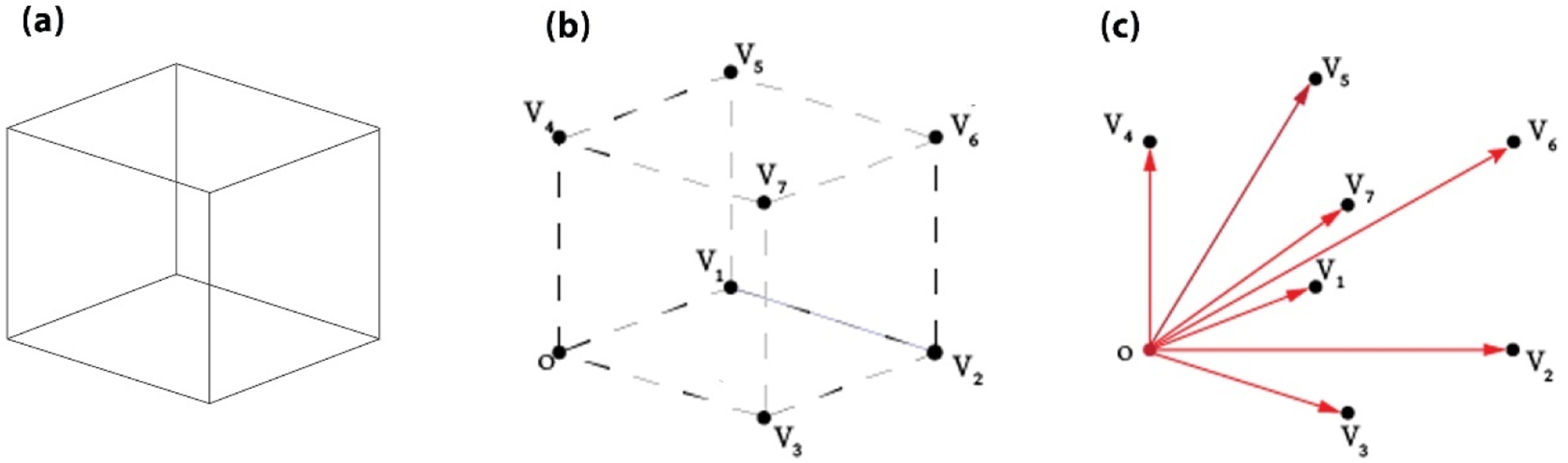

Figure 1(c) shows the 3D visibility graph G (V, E) of G1.

According to the 3D directed graph of G1 in Figure 1(c), the degrees of the vertices are as follows:

\deg^{-} (V_{1}) = \deg^{-} (V_{2}) = \deg^{-} (V_{3}) = \deg^{-} (V_{4}) = \deg^{-} (V_{5}) = \deg^{-} (V_{6}) = \deg^{-} (V_{7}) = 1

\deg^{+} (V_{1}) = \deg^{+} (V_{2}) = \deg^{+} (V_{3}) = \deg^{+} (V_{4}) = \deg^{+} (V_{5}) = \deg^{+} (V_{6}) = \deg^{+} (V_{7}) = 0

\deg^{-} (O) = 0

\deg^{+} (O) = 1

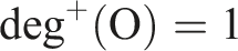
Deg⁺ represents the outdegree of a node; if it is greater than 0, the node can see the environment. If it is 0, the node is not an observer and cannot see. Deg^- represents the indegree of a node; if it is greater than 0, the node is being seen, whereas if it is 0, the node is not visible.

In G1, there is an indegree of visible vertices of 1 and an outdegree of visible vertices of 0, indicating that these points are not observers. In contrast, the indegree of vertex O is equal to zero, whereas its outdegree is equal to 1, indicating that this point has observing characteristics. In other words, the indegree value indicates the level of visibility at a vertex, whereas the outdegree value indicates the level of observation.

To facilitate the interpretation of the resulting 3D visibility graphs, bar-visibility representations are used as a schematic visualization technique (Brandenburg, 2014; Slettnes, 2021). Horizontal line segments (called “vertex segments or bars”) represent the vertices of a graph, and vertical line segments (called “edge segments”) represent its edges (Wang and He, 2012).

In Figure 2, a bar visibility representation of G1 is presented.

Figure 2.

Planar visibility representation of G1.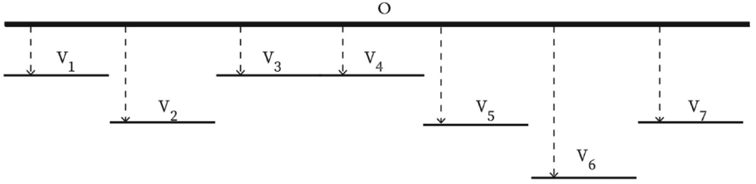

Given that examining intervisibility and locomotion is important in analyzing human environmental perception, considering the pedestrian movement to map visibility produces a more realistic analysis of environmental perception. Therefore, in the cube space, we assume that a pedestrian can be located in O₁, O₂, O_3, and O₄, as shown in Figure 3(a). In this case, the lower points are occupiable, and the upper points are visible. Assuming there is no visibility obstruction between the vertices, the 3D visibility graph G2 accrues as shown in Figure 3(b). The line graph presents visibility values for each observation node in the 3D visibility graph. Nodes are plotted sequentially according to their graph index and do not necessarily represent a continuous pedestrian movement path. Observation nodes (O) indicate spatial locations where an observer can potentially be located and act as a vantage point; however, a pedestrian does not necessarily traverse all observation nodes during movement.

Figure 3.

(a) In the cubic space, O1, O2, O3, and O4 are considered occupiable vertices; V1, V2, V3, and V4 are visible points in the visibility analysis. (b) 3D visibility graph G2 showing the pattern of connections.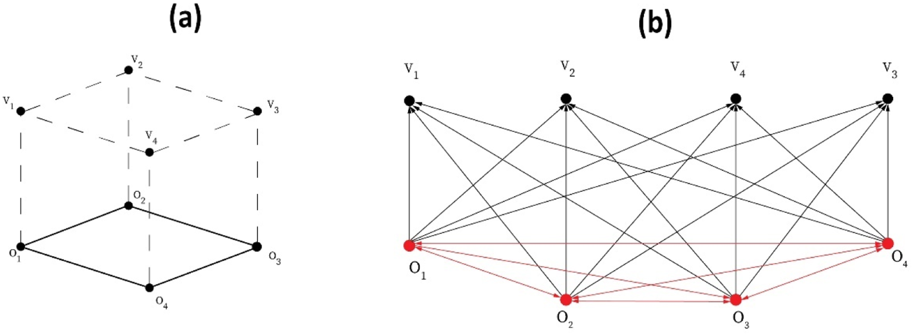

The degree of the vertices of G2 is as follows:

\deg^{-} (V_{1}) = \deg^{-} (V_{2}) = \deg^{-} (V_{3}) = \deg^{-} (V_{4}) = 4

\deg^{+} (V_{1}) = \deg^{+} (V_{2}) = \deg^{+} (V_{3}) = \deg^{+} (V_{4}) = 0

\deg^{-} (O_{1}) = \deg^{-} (O_{2}) = \deg^{-} (O_{3}) = \deg^{-} (O_{4}) = 3

\deg^{+} (O_{1}) = \deg^{+} (O_{2}) = \deg^{+} (O_{3}) = \deg^{+} (O_{4}) = 7

The sum of the outdegree and the indegree is equal to 7, which means that there is an observer point for every visible point:

\sum_{v \in V} \deg - (v) = 7 = \sum_{v \in V} \deg^{+} (v)

Definitely, the representation of the visibility relationship between vertices becomes more complicated with the expansion of the 3D grid in space, such that bar visibility representation is useful in presenting 3D visibility graphs. It should be noted that this representation is not distance-based, emphasizing the connectivity and relational structure between nodes in a clearer and more readable form. Figure 4 shows visibility representation in G2.

Figure 4.

1-Bar visibility representation of G2.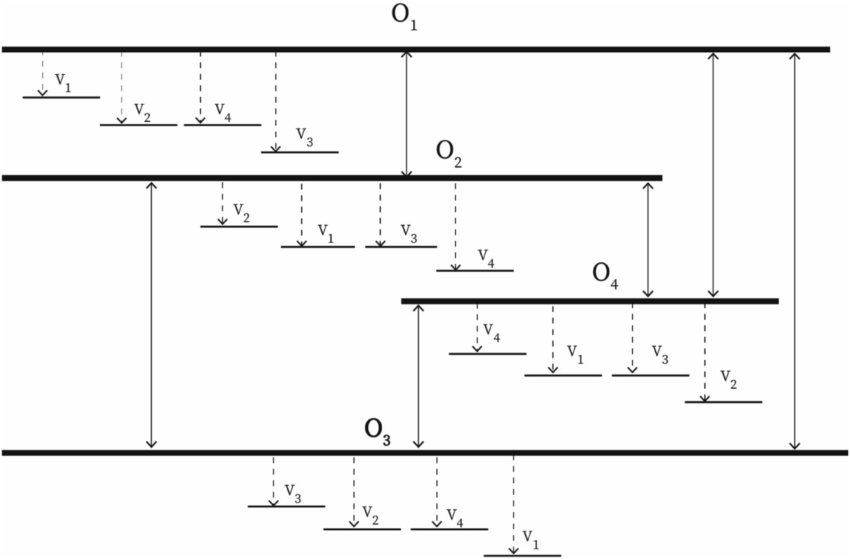

Based on the construction of the targeted 3D visibility graph, three values are calculated: targeted connectivity,¹ targeted integration² (closeness centrality), and targeted connectivity index³ (degree centrality). In 3D, researchers can investigate various research situations based on the visibility graph, from describing the spatial properties of complex architectural designs to describing human cognition and behavior (Lu et al., 2019).

As shown in Figures 3 and 4, in an environment, the relationship between nodes is not solely determined by outdegree and indegree. Other factors, such as distance, can further define the connections between nodes. As it is clear in the figures, the distance of this connection is different from one node to another. This limitation motivates the introduction of a weighted 3D visibility graph, in which inter-node distance is explicitly incorporated as an edge weight.

Methodology

Viewing distance

Distance is a critical parameter in human visual perception, producing distinct qualitative experiences at different scales. Longer sightlines support a wide, panoramic mode of vision, enabling an overall understanding of space, whereas shorter sightlines provide finer visual detail and higher resolution perception. Both contribute unique qualities and cannot be inherently prioritized over one another.

Human-centered urban theories, such as those proposed by Gehl (2010), suggest that short visual distances, particularly at eye level, are closely linked to social interaction potential, while greater distances, although still visually accessible, contribute less to direct engagement. Considering the central field of human vision (approximately 20° vertically and horizontally around the fixation point) (Kruijff et al., 2019), a more distant observer can perceive a larger extent of an object within this visual cone, while a closer observer sees fewer elements but in greater detail (Coors, 2003; Hatfield, 2011; Hyrskykari, 2006; Series and Science, 2019).

Incorporating distance into visibility analysis thus enriches the model by capturing multiple perceptual levels. Distance-based measures do not label distances as inherently “good” or “bad”; instead, they provide a flexible framework that can emphasize overall spatial overview, visual detail, or perceptual intensity (Figure 5), depending on the analytical objectives.

Figure 5.

Conceptual illustration of viewing distance and central field of view in human visual perception. For a fixed central viewing angle (α ≈ 20°), a longer viewing distance (d₁) allows a larger extent of the target (O₁) to be perceived within the central field of view, supporting panoramic spatial understanding, while a shorter viewing distance (d₂) results in a smaller visible extent (O₂) but enables greater visual detail. The diagram illustrates how distance affects perceptual scale without implying that longer or shorter sightlines are inherently preferable.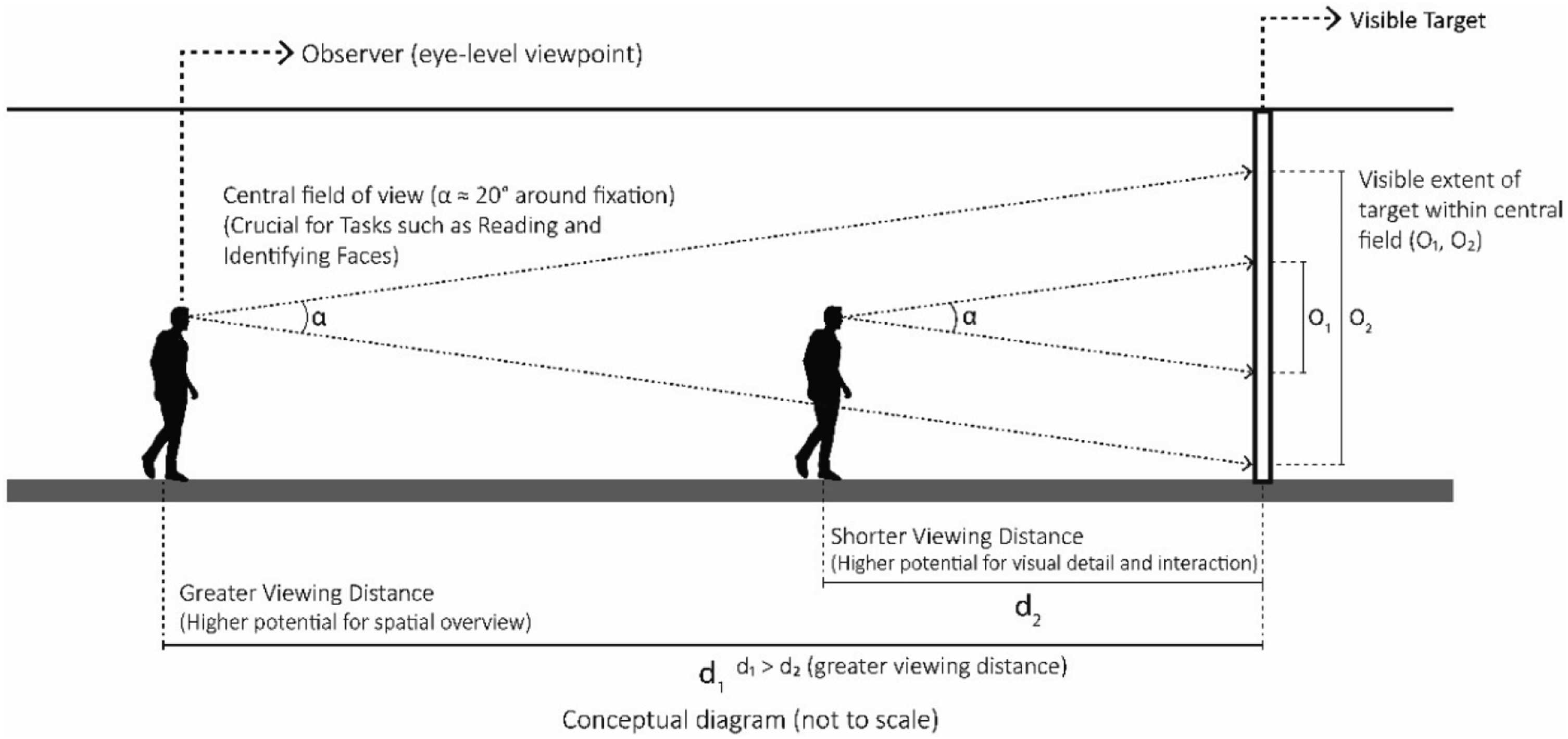

In this study, distance is incorporated as a geometric weighting factor rather than as a calibrated model of human distance perception. The proposed weighting does not assume that perceptual relevance decreases linearly or symmetrically with distance; instead, it provides a transparent, first-order abstraction that makes distance effects explicit within the visibility graph structure. While empirical studies suggest that perceptual relevance may follow non-linear and anisotropic patterns, modeling such effects would require behavioral calibration and is beyond the scope of the present work. The objective here is not to claim perceptual realism, but to extend unweighted visibility graphs by introducing distance as an analyzable spatial parameter.

3D weighted visibility graph

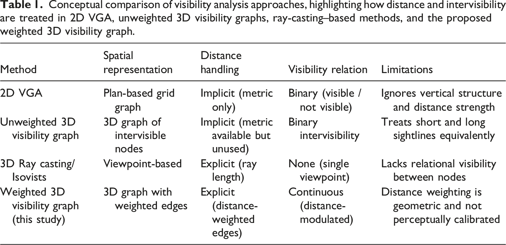
Unlike ray-casting and unweighted visibility graph analysis, which treat all visible connections as equally influential, the proposed weighted visibility graph assigns differential importance to visual connections based on distance along potential movement paths, thereby encoding perceptual priorities rather than purely geometric visibility.

Table 1 summarizes the differences between standard VGA, ray-casting–based visibility analysis, and the proposed weighted visibility graph, clarifying how distance is treated and under what conditions each approach is most informative.

Table 1.

Conceptual comparison of visibility analysis approaches, highlighting how distance and intervisibility are treated in 2D VGA, unweighted 3D visibility graphs, ray-casting–based methods, and the proposed weighted 3D visibility graph.

Method	Spatial representation	Distance handling	Visibility relation	Limitations
2D VGA	Plan-based grid graph	Implicit (metric only)	Binary (visible / not visible)	Ignores vertical structure and distance strength
Unweighted 3D visibility graph	3D graph of intervisible nodes	Implicit (metric available but unused)	Binary intervisibility	Treats short and long sightlines equivalently
3D Ray casting/Isovists	Viewpoint-based	Explicit (ray length)	None (single viewpoint)	Lacks relational visibility between nodes
Weighted 3D visibility graph (this study)	3D graph with weighted edges	Explicit (distance-weighted edges)	Continuous (distance-modulated)	Distance weighting is geometric and not perceptually calibrated

As an observer moves through the environment, they perceive it spatially. Given this fundamental concept, intervisibility plays a crucial role in visibility analysis. Intervisibility refers to mutual visibility—whether graph nodes can see each other or not—and is represented as graph edges in a 3D visibility graph. However, previous theories primarily focus on the existence or absence of mutual visibility or direction of visibility, without addressing the qualitative aspects of this relationship. One key characteristic, viewing distance, is the focus of this paper and forms the basis of the proposed weighted 3D visibility graph.

In this paper, our goal is to develop a 3D visibility graph by defining a weight for the graph’s edges. Referring back to Figure 1, the node pairs O-V₁ and O₁-V₆ have the same degree. However, the relationships between these pairs differ because the nodes are at different distances. In other words, V₁ is visible at a closer distance to O than V₆.

Figure 6 shows the comparison between the conventional 3D visibility graph and the weighted 3D visibility graph. If we consider the distance between O₁ and O₂ to be 1 m, their adjacency matrix clarifies this information, indicating that the weighted 3D visibility graph provides a more accurate and detailed representation of environmental visibility.

Figure 6.

(a) Hypothetical cubic space considered for analysis with visible nodes and observation nodes. (b) Conventional 3D visibility graph with its adjacency matrix. (c) The weighted 3D visibility graph with its adjacency matrix, where longer edges are represented with greater thickness. The sequence of nodes shown in the graphs does not necessarily represent a pedestrian trajectory, but an ordered sampling of visibility values across the spatial graph.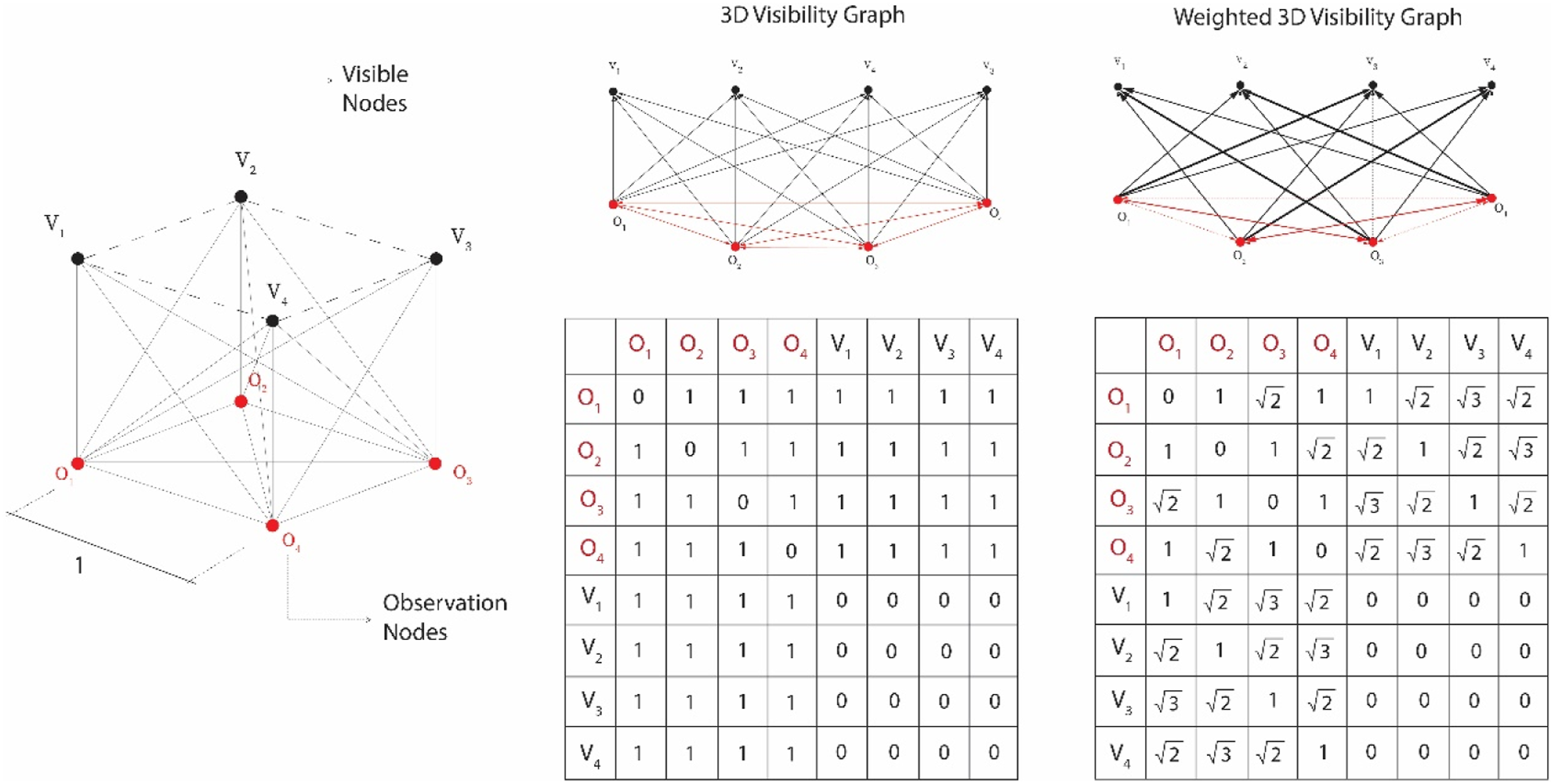

Case study

In this section, the prayer house in Tehran’s Laleh Park has been examined as a case study. This building consists of two nested simple cubes, one inside the other. In terms of the cubes’ openings and rotation of the inner cube, creating a unique visibility pattern.

Figure 7 shows a 3D model of the building, modeled using Rhino 8 software. As presented in the figure, a network of graph nodes has been mapped throughout the building to encompass all its parts. Then, the observation nodes and visible nodes were separated. Bidirectional edges were established between the observation nodes, while unidirectional edges connected the observation nodes to the visible nodes. No edges were formed between the visible nodes themselves. Finally, each edge was assigned a weight corresponding to its length, representing the distance between connected nodes.

Figure 7.

A 3D model of the Laleh Park prayer building, where edges of the weighted 3D visibility graph represent intervisibility relationships between observation and visible nodes. One of the observation nodes has been selected as a sample node to illustrate its visibility relationships with surrounding visible nodes within the weighted 3D visibility graph. Edge thickness is proportional to edge length (distance), indicating higher graph weights. These edges do not represent ray-casting or sampled lines of sight.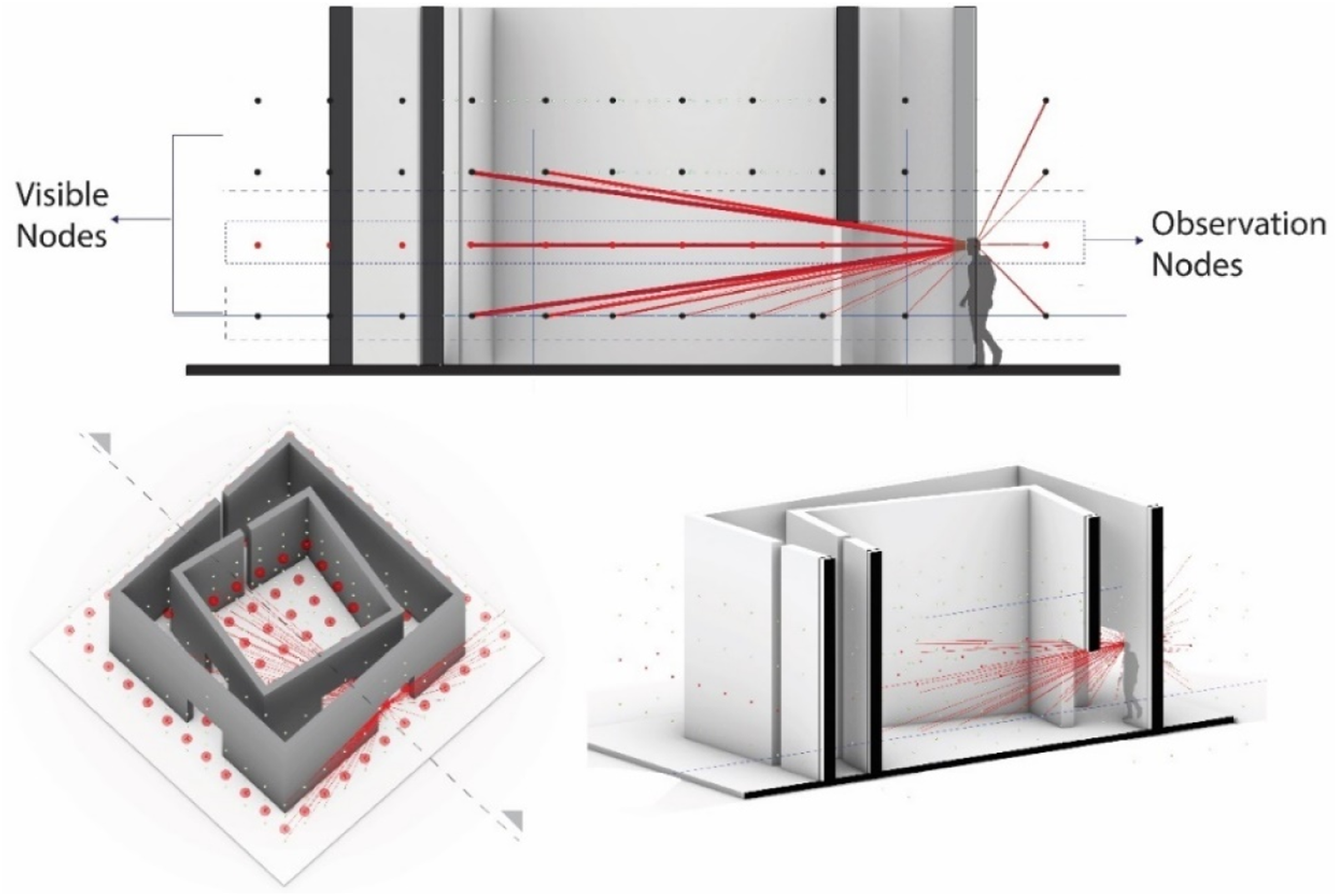

In the pavilion case study, weighted visibility values are evaluated along pedestrian movement paths rather than at isolated viewpoints. This allows the analysis to reveal how perceived openness and visual engagement evolve sequentially during movement, highlighting perceptual differences that are not captured by conventional visibility measures.

One of the nodes has been selected as a sample node to illustrate the relationship between the observation node and the visible nodes.

According to Figure 8(a)–(d), it can be concluded that (a) and (b) alone do not fully represent the relationships between the nodes in the 3D visibility graph, while (c) and (d) provide additional environmental features. Additionally, in graph (e), the values of all four parameters are compared after normalization, highlighting the differences in each observation node.

Figure 8.

(a), (b), (c), and (d) present the heatmaps and dot plot for 3D Connectivity, 3D Integration, 3D Sum of Distance, and 3D Average Distance of the observation nodes in the case study; (e) compares the four values, 3D Connectivity, 3D Integration, and 3D Sum of Distance, to highlight their variations. The dot plots illustrate the distribution of metric values across observation nodes.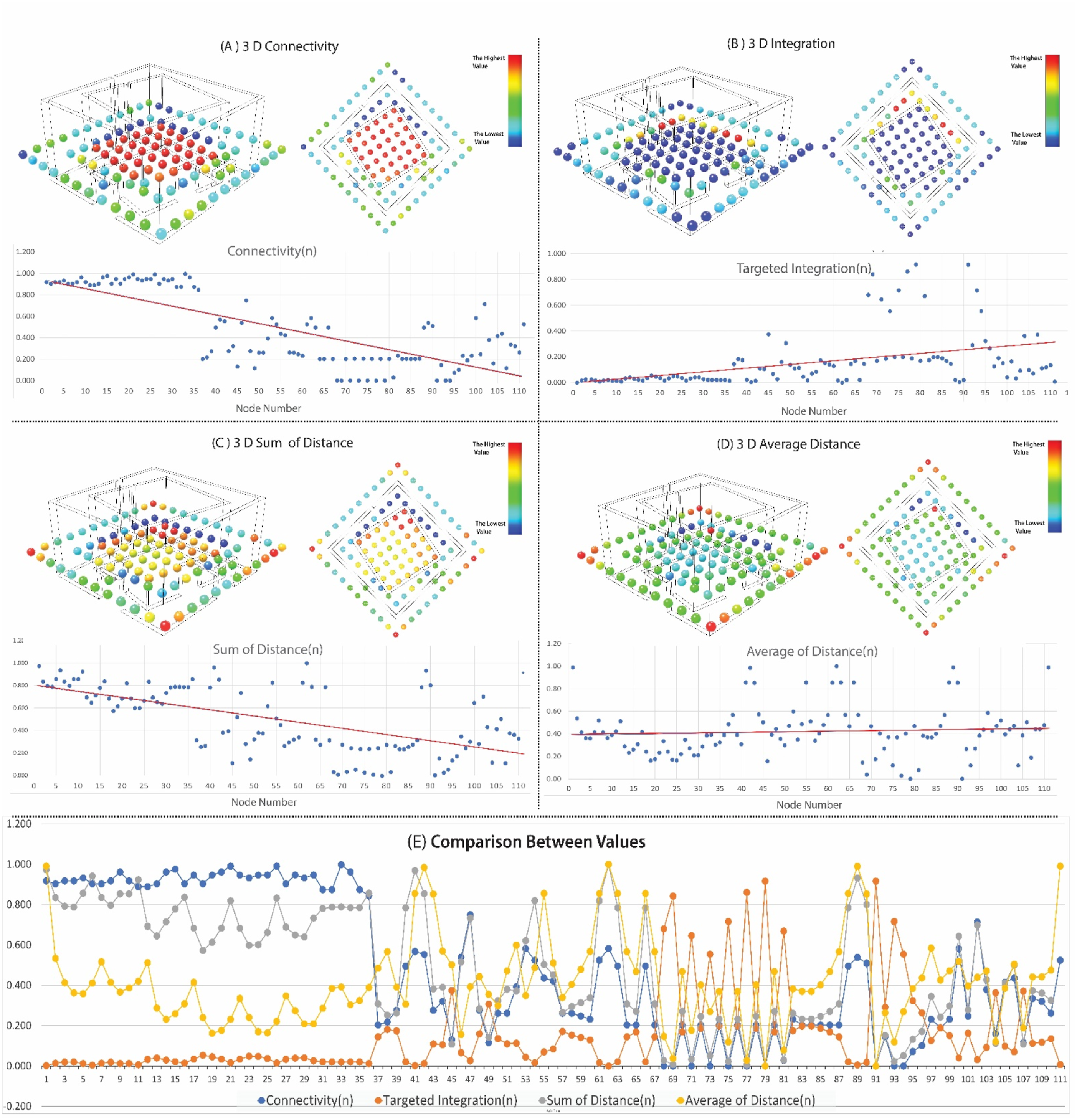

Conventionally, these factors are calculated in a 3D visibility graph. However, by incorporating distance-based weights in the weighted 3D visibility graph, additional factors can be analyzed. One such factor is the set of distances (or weights) at each observation node, along with the average distance, which is determined by the sum of distances to the outdegree of the observation nodes.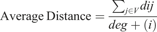

Average Distance = \frac{\sum_{j \in V} d i j}{\deg + (i)}

Where dij is the weighted distance between observation node $i$ and visible node $j$ . deg+( $i$ ) is the outdegree of the observation node $i$ (i.e., the number of visible nodes connected to it). V is the set of observation nodes connected to the visible node.

The average distance metric quantifies the average visibility reach of a node. In an unweighted 3D visibility graph, this would be equivalent to the visible neighboring nodes in a graph. A weighted graph incorporates distance perception, making it a more informative representation of spatial visibility reach. Unlike integration or connectivity, Average Distance provides localized information about how far a node can “see.” Unlike connectivity, which only represents the number of visible nodes, Average Distance describes the typical spatial reach of visibility from an observation node. Dividing the total distance by the number of visible nodes normalizes the metric, allowing comparison between nodes with different visibility counts and preventing highly connected nodes from automatically producing larger values.

Results and discussion

In this section, four values, Connectivity, Integration, Sum of Distance, and Average Distance, were calculated for the case study using the Grasshopper Plugin. Figure 8 presents a comparison of these values. All heatmaps illustrate the values relative to the observation nodes, with visible nodes that were not shown in the figure to enhance the clarity of the observation node distribution.

According to Figure 8, the central part of the plan has the highest connectivity and the lowest integration, while the sum of distances and average distance are relatively low. Thus, these metrics extend conventional visibility analysis by revealing distance-sensitive variations.

While Connectivity and Integration primarily describe the topological structure of visibility relations, Sum of Distance and Average Distance additionally capture the spatial extent of visibility. As a result, observation nodes with similar connectivity values may still differ in the distance distribution of their visible nodes. These differences reveal variations in perceptual scale and visibility reach that are not represented in conventional unweighted visibility analysis. For example, at node 88, Connectivity and Integration are relatively high, while Average Distance and Sum of Distance remain comparatively low. This divergence demonstrates that the proposed metrics capture additional aspects of spatial visibility beyond conventional graph measures.

Figure 9 presents the variation of 3D Connectivity, 3D Integration, 3D Sum of Distance, and 3D Average Distance along a selected path in space. The line graphs show that, although these metrics are evaluated along the same path, they capture different aspects of spatial visibility. In particular, the values of 3D Sum of Distance and 3D Average Distance diverge at specific locations along the path, indicating that each metric provides a distinct analytical perspective on visual conditions rather than redundant information. In this sense, since observers experience architectural space continuously rather than discretely, analyzing the metrics along a path helps describe how visual conditions vary during movement through the environment.

Figure 9.

(a) Top view of an observer’s path in the environment. (b) Linear graph of the four values: 3D Connectivity, 3D Integration, and 3D Sum of Distance along the path. (c) 3D view of the visibility graph formed at point 8, shown as a representative observation node to illustrate local edge relationships.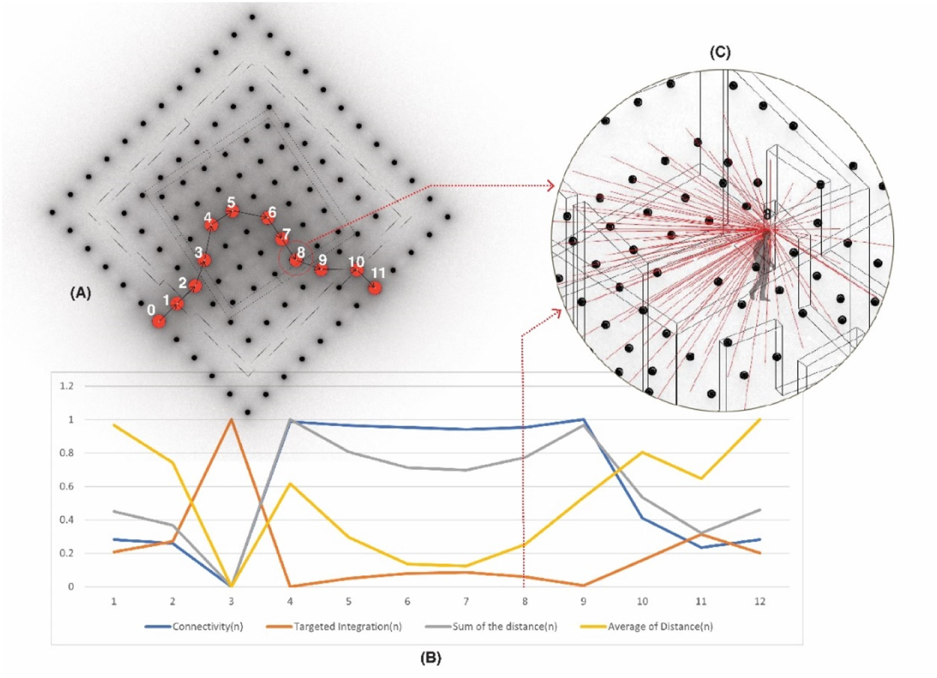

The proposed model does not prioritize distant or close views in terms of preference; instead, it captures how visibility intensity varies with distance. Questions related to subjective visual preference, such as whether a distant preferred view should outweigh a closer, less preferred one, may be addressed in future work by integrating additional semantic or perceptual weighting layers.

Conclusion

Although visibility analysis has recently been found to be highly successful in the 3D environment, some features of the environment have been ignored, among which are locomotion and visual interaction. Accordingly, we proposed an updated model for 3D visibility graph.

The method provides an explanatory framework for analyzing visibility relations under movement-related conditions, rather than a simulation of pedestrian motion or visual preference.

In conventional visibility graphs, the relationship between nodes was solely defined by the presence or absence of a connection, serving as the basis for mutual visibility analysis. However, this study introduces an additional layer of information by considering the quality of the connection between visibility nodes in terms of visibility distance. Consequently, this paper presents the weighted 3D visibility graph, which enhances visibility analysis accuracy by incorporating distance as a fundamental parameter.

First, a 3D visibility graph was constructed in the case study environment of the prayer house in Tehran’s Laleh Park. Then, a weight equivalent to the edge length was considered for each edge. Next, two new metrics, Average Distance and Sum of Distances, were introduced and calculated for each observation node. By comparing these metrics with conventional 3D graph analysis measures, Connectivity and Integration, the weighted 3D visibility graph revealed additional insights into visibility relations, including differences in spatial visibility reach, and distinctions between observation nodes that exhibit similar topological visibility properties but different distance distributions.

Further research can explore the potential of this model by applying it to more complex case studies. To enhance spatial analysis, other advanced metrics, such as Weighted Integration (3D) and Weighted Clustering Coefficient, may also be developed and extended within the framework of a weighted 3D visibility graph.

Footnotes

Sara Omraniazizabad

Mohammadjavad Mahdavinejad

Funding

The authors received no financial support for the research, authorship, and/or publication of this article.

Declaration of conflicting interests

The authors declared no potential conflicts of interest with respect to the research, authorship, and/or publication of this article.

Data Availability Statement

The datasets used and/or analyzed during the current study are contained within the manuscript. No additional datasets were generated or analyzed beyond those included in the article.

Notes

Author biographies

Sara Omraniazizabad is a Master of Architecture and a researcher at the High-Performance Architecture Research Cluster, College of Engineering and Architecture, University of Nizwa, Oman, and the Faculty of Art and Architecture, Tarbiat Modares University, Tehran, Iran. Her research focuses on AI-powered design and planning, agent-based modeling, spatial analysis, spatial decision support systems (SDSS), and digital twin technologies. She has been involved in the development of a human-centered digital twin platform, focusing on modeling navigation, perception, and movement behavior in built environments through computational methods, coding, and data-driven analysis.

Professor Mohammadjavad Mahdavinejad is focused on High-performance Architecture. The Highperformance Architecture Theory advocates a designerly approach to complex science–technology phenomena in architectural design and practice, including carbon neutrality water–energy efficiency, visual-thermal comfort, and a mathematical–systemic understanding of architecture and design process. He is the founder of HAL (High-performance Architecture Laboratory) in Iran, the HARec (Highperformance Architecture Research Cluster) in Oman, and GRACE in Germany. He is currently a professor at the College of Engineering and Architecture, University of Nizwa, Oman.

References

Austern

Yosifof

Michaeli

, et al. (2025) Convolutional neural networks for predicting the perceived density of large urban fabrics. Computers, Environment and Urban Systems 120: 102304. https://doi.org/10.1016/j.compenvurbsys.2025.102304

Batty

(2001) Exploring isovist fields: space and shape in architectural and urban morphology. Environment and Planning B: Planning and Design 28(1): 123–150. https://doi.org/10.1068/b2725

Benedikt

(1979) To take hold of space: isovists and isovist fields. Environment and Planning B: Planning and Design 6(1): 47–65. https://doi.org/10.1068/b060047

Bhatia

Chalup

Ostwald

(2012) Analyzing Architectural Space: Identifying Salient Regions by Computing 3D Isovists. 46th Annual Conference of the

Architectural Science Association (ANZAScA

2012).

Bishop

(2003) Assessment of visual qualities, impacts, and behaviours, in the landscape, by using measures of visibility. Environment and Planning B: Planning and Design 30(5): 677–688. https://doi.org/10.1068/b12956

Boomari

Zarei

(2022) Visibility graphs of anchor polygons. Journal of Graph Algorithms and Applications 26(1): 15–34. https://doi.org/10.7155/jgaa.00579

Brandenburg

(2014) 1-Visibility representations of 1-Planar graphs. Journal of Graph Algorithms and Applications 18(3): 421–438. https://doi.org/10.7155/jgaa.00330

Coors

(2003) Graphical Abstraction and Progressive Transmission in Internet-based 3D- Geoinformationsystems. Technical University of Darmstadt.

Dalton

(2015) The problem of representation of 3D isovists. Proceedings of the 10th International Space Syntax Symposium. 1–18.

10.

Davis

Benedikt

(1979) Computational models of space: isovists and isovist fields. Computer Graphics and Image Processing 11(1): 49–72. https://doi.org/10.1016/0146-664X(79)90076-5

11.

Fisher-Gewirtzman

(2018) Integrating ‘weighted views’ to quantitative 3D visibility analysis as a predictive tool for perception of space. Environment and Planning B: Urban Analytics and City Science 45(2): 345–366. https://doi.org/10.1177/0265813516676486

12.

Fisher-Gewirtzman

Natapov

(2014) Different approaches of visibility analyses applied on hilly urban environment. Survey Review 46(338): 366–382. https://doi.org/10.1179/1752270614Y.0000000117

13.

Fisher-Gewirtzman

Shach-Pinsly

Wagner

, et al. (2005) View-oriented three-dimensional visual analysis models for the urban environment. Urban Design International 10(1): 23–37. https://doi.org/10.1057/palgrave.udi.9000133

14.

Fisher-Gewirtzman

Yosifof

Dalyot

(2019) Visual experience route calculation algorithm for urban environments. Proceedings of the 12th International Space Syntax Symposium 2019.

15.

Gehl

(2010) Cities_For_People. Island Press.

16.

Gibson

(1979) The Ecological Approach to Visual Perception. Boston: Houghton Mifflin Company.

17.

Hardy

(1967) Landscape and human perception. In: Murray

(ed) Methods of Landscape Analysis. Landscape Research Group, pp. 3–8 Volume October.

18.

Hatfield

(2011) Philosophy of Perception and the Phenomenology of Visual Space. Philosophic Exchange, 42, 31–66.

19.

Hillier

Bill

Hanson

Julienne

(1984) The Social Logic of Space. Cambridge University Press, Cambridge.

20.

Hillier

Major

Desyllas

, et al. (1996) Tate Gallery, Millbank: A Study of the Existing Layout and New Masterplan Proposal. The bartlett School of Graduate Studies, 1–15. Available at: https://eprints.ucl.ac.uk/932.

21.

Hyrskykari

(2006) Aulikki Hyrskykari Eyes in Attentive Interfaces: Experiences from Creating iDict, a Gaze-Aware Reading Aid. University of Tampere: Dissertations in Interactive Technology.

22.

Kim

(2019) A new 3D space syntax metric based on 3D isovist capture in urban space using remote sensing technology. Computers, Environment and Urban Systems 74(April 2018): 74–87. https://doi.org/10.1016/j.compenvurbsys.2018.11.009

23.

Kondyli

Bhatt

Hartmann

(2018) Precedent based design foundations for parametric design: the case of navigation and wayfinding. Advances in Computational Design 3(4 Special Issue): 339. https://doi.org/10.12989/acd.2018.3.4.339

24.

Kruijff

Orlosky

Kishishita

, et al. (2019) The influence of label design on search performance and noticeability in wide field of view augmented reality displays. IEEE Transactions on Visualization and Computer Graphics 25(9): 2821–2837. https://doi.org/10.1109/TVCG.2018.2854737

25.

Krukar

Schultz

Bhatt

(2017) Towards embodied 3D isovists. Incorporating cognitively-motivated semantics of `space’ and the architectural environment in 3D visibility analysis. Proceedings of the 11th Space Syntax Symposium, 1–13.

26.

Krukar

Manivannan

Bhatt

, et al. (2020) Embodied 3D isovists: a method to model the visual perception of space. Environment and Planning B: Urban Analytics and City Science 48(8): 1–19. Available at: https://doi.org/10.1177/2399808320974533

27.

Lonergan

Hedley

(2016) Unpacking isovists: a framework for 3D spatial visibility analysis. Cartography and Geographic Information Science 43(2): 87–102. https://doi.org/10.1080/15230406.2015.1065761

28.

Gou

, et al. (2019) Three-dimensional visibility graph analysis and its application. Environment and Planning B: Urban Analytics and City Science 46(5): 948–962. https://doi.org/10.1177/2399808317739893

29.

Omrani Azizabad

Mahdavinejad

Hadighi

(2024) Three-dimensional embodied visibility graph analysis: investigating and analyzing values along an outdoor path. Environment and Planning B: Urban Analytics and City Science 52: 23998083241303200. https://doi.org/10.1177/23998083241303199

30.

Ostwald

Dawes

(2020) Isovists: Spatio-visual mathematics in architecture. Handbook of the Mathematics of the Arts and Sciences, 1–13. Available at: https://doi.org/10.1007/978-3-319-70658-0_5-3

31.

Series

IOPC

Science

(2019) Based on creative thinking to museum lighting design influences to visitors emotional response levels theory research based on creative thinking to museum lighting design influences to visitors emotional response levels theory. https://doi.org/10.1088/1757-899X/573/1/012093

32.

Slettnes

(2021) Minimal embedding dimensions of rectangle k-visibility graphs. Journal of Graph Algorithms and Applications 25(1): 59–96. https://doi.org/10.7155/JGAA.00550

33.

Suleiman

Joliveau

Favier

(2013) A new algorithm for 3D isovists. Advances in Geographic Information Science: 157–173. https://doi.org/10.1007/978-3-642-32316-4_11

34.

Tandy

CRV

(1967) The isovist method of landscape survey. In: Murray

(ed) Methods of Landscape Analysis. Landscape Research Group, pp. 9–10.

35.

Turner

Doxa

O’Sullivan

, et al. (2001) From isovists to visibility graphs: a methodology for the analysis of architectural space. Environment and Planning B: Planning and Design 28(1): 103–121. https://doi.org/10.1068/b2684

36.

Varoudis

Psarra

(2014) Beyond two dimensions: architecture through three-dimensional visibility graph analysis. The Journal of Space Syntax 5(1): 91–108.

37.

Wang

(2012) Visibility representation of plane graphs with simultaneous bound for both width and height. Journal of Graph Algorithms and Applications 16(2): 317–334. https://doi.org/10.7155/jgaa.00260

38.

Watts

Strogatz

(1998) Watts_Strogatz_Collective_dynamics_small_world_networks.1998. Nature 393(June): 440–442.

39.

Wiener

Franz

(2005) Isovists as a means to predict spatial experience and behavior. Lecture Notes in Artificial Intelligence (Subseries of Lecture Notes in Computer Science) 3343(June): 42–57. https://doi.org/10.1007/978-3-540-32255-9_3

40.

Yosifof

Austern

Fisher-Gewirtzman

(2024) Macro-scale urban spatial openness index (USOI) predicting the perceived density of various urban morphologies. Proceedings of the 14th International Space Syntax Symposium, Cyprus 24-27 June 2024.