The spatial interactions among the neighborhoods of Dijon Métropole,France: A comparative analysis

Abstract

This paper makes a methodological contribution to the field of hierarchical-spatial models applied to housing prices by addressing the nature of spatial interaction at higher levels of analysis. While spatial interactions at the dwelling level are often straightforward to model, spatial processes at the neighborhood level are more abstract, serving as proxies for latent constructs such as neighborhood quality. The present study builds on the distinction between endogenous and exogenous interaction effects, as well as global and local spillovers, to compare three upper-level interaction structures: endogenous (HSAR), exogenous (HSLX), and mixed (HSDM). A Bayesian estimation strategy is employed in conjunction with the Deviance Information Criterion (DIC) to evaluate these specifications using 6566 housing transactions in Dijon Métropole, France, between 2013 and 2017. The findings of this study suggest that models incorporating endogenous upper-level dependence provide a superior fit to the data in comparison to the purely exogenous alternative. However, the distinction between global and mixed spillovers necessitates a meticulous evaluation. While the complete DIC provides slight support for the endogenous model, the conditional DIC and the lack of statistical significance for the autoregressive coefficient in the mixed specification provide stronger evidence for the HSAR model as the more parsimonious and appropriate representation of spatial dependence.

Keywords

multilevel modeling spatial econometrics property prices local spatial analysis spatial interactions

Introduction

Housing prices are shaped by processes operating across multiple spatial scales, ranging from the characteristics of individual dwellings to the broader neighborhood dynamics. This calls for models that can accommodate both hierarchy and spatial dependence. Hierarchical-spatial models offer a natural framework for the analysis of such processes. Lower-level units (e.g., dwellings) are nested within higher-level units (e.g., neighborhoods or municipalities), while spatial dependence may arise at one or several levels of the hierarchy (Beron et al., 1999; Djurdjevic et al., 2008; Gelfand et al., 2007; Glaesener and Caruso, 2015; Huang and Clark, 2002; Jones, 1991; Moreira De Aguiar et al., 2014; Orford, 2000, 2002).

However, in the context of housing data, the interpretation of spatial structure is not straightforward at all levels of analysis. At the level of individual properties, distances and contiguities are typically directly observable. Conversely, at higher levels of analysis, such as neighborhoods or municipalities, conceptualizing spatial dependence becomes more challenging. This is due to the fact that spatial dependence often reflects latent and only partially observed dimensions, such as neighborhood quality. The selection of upper-level spatial specification is not merely a technical modeling issue; it is also a matter of how neighborhood effects are conceptually understood.

A useful point of departure is the distinction between endogenous and exogenous interaction effects in the sense of Manski (2000), together with the distinction between global and local spillovers. Endogenous effects arise when the outcome observed in a specific spatial unit is influenced by outcomes in proximate units, thereby inducing feedback mechanisms that may disseminate throughout the broader spatial system. These effects are generally represented by spatial autoregressive processes and can be interpreted as global spillovers. Conversely, exogenous effects are attributed to the characteristics of neighboring units and are typically modeled through spatially lagged covariates. These effects are more naturally interpreted as local spillovers. A combination of both mechanisms is achieved by means of mixed specifications. (Anselin, 2022; LeSage and Pace, 2008, 2014; Vega and Elhorst, 2013).

In the field of housing literature, this distinction holds particular significance at the neighborhood level. Existing studies on hierarchical-spatial organization have predominantly focused on endogenous interaction structures. For instance, Dong et al. (2015) utilized a two-level hierarchical-spatial model with SAR processes at both levels to analyze the land market in Beijing, China. In a comparative setting, Cellmer et al. (2019) demonstrated that a hierarchical-spatial autoregressive specification outperformed classical linear, multilevel, and SAR models. The HSAR random intercept model for Liverpool, England, was estimated by Dong et al. (2019), while Pérez-Molina (2022) combined HSAR and hierarchical CAR specifications in San José, Costa Rica. In other studies, lagged covariates have been utilized, particularly in the works by Chasco and Le Gallo (2013) on Madrid, Nordvik et al. (2019) on Oslo and Hall et al. (2022) on the state of Ohio, U.S.A. Nevertheless, a compelling justification for the adoption of distinct spatial specifications remains absent.

This paper addresses that gap by explicitly comparing three upper-level specifications within a two-level hierarchical-spatial framework. The initial specification is a hierarchical SAR model (HSAR), which represents endogenous global spillovers. The second model is a hierarchical SLX model (HSLX), which captures exogenous local spillovers through neighborhood covariates. The third is a hierarchical state-dependent model (HSDM), which combines both mechanisms. A Bayesian estimation strategy, in conjunction with model comparison based on the Deviance Information Criterion (DIC, Spiegelhalter et al., 2002), was employed to evaluate these competing specifications using a dataset of 6566 dwelling transactions in Dijon Métropole, France, between 2013 and 2017. The contribution of the paper is twofold: it compares alternative models and demonstrates that different upper-level spatial specifications correspond to distinct conceptual views of neighborhood quality. The empirical findings indicate that while exogenous neighborhood spillovers are present, the evidence favors specifications that allow for endogenous upper-level interaction. Specifically, the HSAR model is identified as the most compelling representation. This conclusion is supported by two factors. First, the HSAR model demonstrates superior performance under the conditional DIC. Second, the spatial autoregressive parameter exhibits statistical robustness. This parameter remains significant in the HSAR specification but loses significance once additional exogenous interactions are introduced in the mixed model. The paper thus emphasizes the importance of aligning the conceptual definition of upper-level spatial processes with their econometric specification.

The remainder of the paper is organized as follows. Section 2 describes the hierarchical-spatial models and their estimation method. Section 3 describes the data and variables used in this study. Section 4 presents and discusses the estimation results. Finally, section 5 concludes with a brief summary of the findings and discussions on potential limitations of the study.

Methodology

Hierarchical-spatial models

Classical multilevel models are unable to fully capture spatial autocorrelation, underscoring the necessity for the development of appropriate multilevel spatial models (Chasco et al., 2012). To study both the hierarchical and spatial dimensions of the data, it is necessary to employ a hierarchical-spatial approach. Corrado and Fingleton (2012) argue for the integration of multilevel and spatial modeling into econometric models, demonstrating that the spatial dimension is inherent to the structure of hierarchical models. Furthermore, according to the same authors, multilevel modeling also differs advantageously from the use of regional or country dummy variables. Consequently, multilevel models have incorporated spatial dependencies, thereby creating hierarchical-spatial models.

This study introduces the two-level hierarchical structure by a varying intercept (Gelman et al., 2014) at the lower-level. Spatial dependence is introduced through spatial regression models at the upper level. These models are designated as HSAR (Hierarchical SAR), HSLX (Hierarchical SLX) or HSDM (Hierarchical SDM). The HSEM (Hierarchical SEM) is not considered in this context, as the SDM can be seen as a rewriting of the SEM as described by LeSage and Pace (2008).

Consider a set of N observed real estate transactions, denoted as y_i with i = 1, …, N, and J level-2 units. The hierarchical-spatial models are expressed in matrix form as follows:

1. HSAR:

\begin{align} L e v e l - 1 : y & = X β + V α + ϵ \end{align}

(1a)

\begin{align} L e v e l - 2 : α & = ρ W α + Z γ + u \end{align}

(1b)

2. HSLX:

\begin{align} L e v e l - 1 : y & = X β + V α + ϵ \end{align}

(2a)

\begin{align} L e v e l - 2 : α & = Z γ + W Z θ + u \end{align}

(2b)

3. HSDM:

\begin{align} L e v e l - 1 : y & = X β + V α + ϵ \end{align}

(3a)

\begin{align} L e v e l - 2 : α & = ρ W α + Z γ + W Z θ + u \end{align}

(3b)

where y is the N × 1 vector of transaction prices, X is an N × k matrix of property-level variables and V is a N × J random effect design matrix. β is a k × 1 vector of coefficients to be estimated. ϵ is a N × 1 lower-level vector of disturbances: ϵ ∼ (0; σ²I_N) where I_N is the N × N identity matrix.

The upper-level of the hierarchical structure depicts and estimates the quality of each neighborhood introduced at level-1 by the J × 1 vector α. Z is a J × (m + 1) matrix of neighborhood-level characteristics (such as amenities, pollution or population density). γ and θ are the J × m vectors of coefficients to be estimated. u is the J × 1 vector of disturbances: u ∼ (0; τ²I_J) where I_J is the J × J identity matrix.

W is a J × J spatial weights matrix that encodes the spatial relationships between neighborhoods. In this study, W is a contiguity based spatial weights matrix where w_ij = 1 if two neighborhoods i and j share a common geographic border, 0 otherwise. This type of matrix is commonly used in the field of hierarchical-spatial analysis, as evidenced by the works of Moreira De Aguiar et al. (2014); Dong et al. (2015); Cellmer et al. (2019) and Dong et al. (2019). In this research, the weights are set so that row totals sum to one.

W is a J × J spatial weights matrix that encodes the spatial relationships between neighborhoods. In this study, W is a contiguity based spatial weights matrix where w_ij = 1 if two neighborhoods i and j share a common geographic border, 0 otherwise. This type of matrix is commonly used in the field of hierarchical-spatial analysis, as evidenced by the works of Moreira de Aguiar et al. (2014); Dong et al. (2015); Cellmer et al. (2019) and Dong et al. (2019). In this research, the weights are set so that row totals sum to one.

Conceptual interpretation of upper-level spillovers

Modeling neighborhood quality, α, as a spatial lag model introduces spatial spillovers at the upper level of the hierarchy and thus generating endogenous, exogenous, or mixed feedback effects (Manski, 2000). Once the equations are estimated, marginal effects on prices can be derived. This involves solving the α equation (level-2) in its reduced form and then incorporating it back into the y equation of interest (level-1).

The partial derivatives for these models are as follows:

1. HSAR model:

\begin{align} y & = X β + V α + ϵ \end{align}

(4)

where

\begin{align} α & = {(I_{J} - ρ W)}^{- 1} [Z γ + u] \end{align}

(5)

The marginal effects are given by

\begin{align} \frac{\partial y}{\partial x_{k}} & = β_{k} \end{align}

(6)

\begin{align} \frac{\partial α}{\partial z_{m}} & = {(I_{J} - ρ W)}^{- 1} γ_{m} \end{align}

(7)

\begin{align} \frac{\partial y}{\partial z_{m}} & = V {(I_{J} - ρ W)}^{- 1} γ_{m} \end{align}

(8)

2. HSLX model:

\begin{array}{l} Eq. (4) \end{array}

where

\begin{align} α & = Z γ + W Z θ + u \end{align}

(9)

The marginal effects are given by

\begin{array}{l} Eq. (6) \end{array}

\begin{align} \frac{\partial α}{\partial z_{m}} & = γ_{m} + W θ_{m} \end{align}

(10)

\begin{align} \frac{\partial y}{\partial z_{m}} & = V (γ_{m} + W θ_{m}) \end{align}

(11)

3. HSDM model:

\begin{array}{l} Eq. (4) \end{array}

where

\begin{align} α & = {(I_{J} - ρ W)}^{- 1} [Z γ + W Z θ + u] \end{align}

(12)

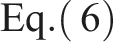
The marginal effects are given by

\begin{array}{l} Eq . (6) \end{array}

\begin{align} \frac{\partial α}{\partial z_{m}} & = {(I_{J} - ρ W)}^{- 1} (γ_{m} + W θ_{m}) \end{align}

(13)

\begin{align} \frac{\partial y}{\partial z_{m}} & = V \{{(I_{J} - ρ W)}^{- 1} (γ_{m} + W Z θ_{m})\} \end{align}

(14)

Equation (6) gives the marginal effect of a dwelling-scale variable (x_k) on the price y. Equations (7), (10), and (13) give the marginal effect of a neighborhood-scale variable (z_m) on the latent district quality α for SAR, SLX, and SDM processes. Equations (8), (11), and (14) are the marginal effects of z_m directly on y via V.

These effects decompose into direct, indirect, and total effects (LeSage and Pace, 2014). Direct effects are defined as the total impact of z_m on α_j itself. This impact is comprised of two components: the “normal” effect, denoted by γ_m, and feedback through the spatial multiplier’s diagonal, symbolized by ${(I - ρ W)}_{j j}^{- 1}$ . Indirect effects constitute global spillovers to other neighborhoods α_l (l ≠ j) via off-diagonal elements ${(I - ρ W)}_{l j}^{- 1}$ , propagating through the entire system beyond immediate neighbors defined by W. In contrast, local spillovers Wθ_m are confined to direct neighbors only.

Thus, beyond their formal definitions, the three specifications embody distinct conceptual views of neighborhood quality. HSAR models random intercepts as an endogenous spatial lag, wherein neighborhood quality emerges from neighboring qualities via global spillovers (Anselin, 2003). HSLX posits quality as local characteristics plus neighboring covariates’ influence (local spillovers), without outcome feedback (Anselin, 2022; LeSage and Pace, 2008, 2014; Vega and Elhorst, 2013). HSDM combines both mechanisms (LeSage and Pace, 2014).

In this framework, the spatial autoregressive parameter, denoted by ρ, in HSAR and HSDM quantifies the intensity of global feedback in the latent quality index. Conversely, the coefficients on spatially lagged covariates, as implemented in HSLX and HSDM, measure the magnitude of local spillovers in observable neighborhood characteristics. The relative magnitude and significance of these parameters indicate whether spatial dependence at the upper level is primarily driven by global feedback or by local diffusion of observed attributes. When the correlation remains substantial and statistically significant even after accounting for the spatial lags of covariates, it suggests that neighborhood quality cannot be reduced to local spillovers in amenities or socio-demographic variables alone.

Bayesian Markov Chain Monte Carlo (MCMC) methods are employed to estimate the hierarchical-spatial models. This approach is particularly well suited to multilevel spatial specifications, as it enables joint inference on regression coefficients, latent neighborhood effects, variance components, and spatial dependence parameters within a unified framework. The Bayesian estimation procedure is implemented in R using bespoke routines developed in nimble. For further discussion of Bayesian hierarchical modeling and MCMC-based inference, consult Gelman and Hill (2006); Banerjee et al. (2014); Gelman et al. (2014) and Dong et al. (2015).

Conditional and complete deviance information criteria

Model comparison is conducted using the Deviance Information Criterion (DIC, Spiegelhalter et al., 2002), which extends information-based model selection to hierarchical Bayesian models estimated by MCMC. Because the HSAR, HSDM, and HSLX specifications differ in their second-level spatial structure, it is useful to distinguish between a conditional DIC and a complete DIC.

In general, the DIC is defined as

D I C = 2 \bar{D (Θ)} - D (\bar{Θ}) = \bar{D (Θ)} + p_{D},

(15)

where

D (Θ) = - 2 \log p (\cdot ∣ Θ) + C,

(16)

$p_{D} = \bar{D (Θ)} - D (\bar{Θ})$ is the effective number of parameters, C is a constant that cancels out in model comparisons, Θ the model’s parameters and log p(⋅|Θ) the log-likelihood function.

The conditional DIC is based on the first-level likelihood only, conditional on the latent level-2 effects:

D_{c} (Θ, θ) = - 2 \log p (y ∣ α, Θ) + C .

(17)

Given the first-level equation

y = X β + V α + ε, ε \sim N (0, σ_{e}^{2} I_{N}),

(18)

The corresponding conditional log-likelihood is

\log p (y ∣ α, Θ) = - \frac{N}{2} \log (2 π) - \frac{N}{2} \log (σ_{e}^{2}) - \frac{1}{2 σ_{e}^{2}} {(y - X β - V α)}^{'} (y - X β - V α) .

(19)

The conditional DIC is then

{D I C}_{c} = 2 \bar{D_{c} (Θ, α)} - D_{c} (\bar{Θ}, \bar{α}) .

(20)

By contrast, the complete DIC is based on the joint density of the observed outcome and the level-2 latent effects:

p (y, α ∣ Θ) = p (y ∣ α, Θ) p (α ∣ Θ),

(21)

so that

D (Θ, α) = - 2 \log p (y, α ∣ Θ) + C,

(22)

and

D I C = 2 \bar{D (Θ, α)} - D (\bar{Θ}, \bar{α}) .

(23)

The distinction matters because the second-level density differs across models. For HSAR,

α = ρ W α + Z γ + u, u \sim N (0, σ_{u}^{2} I_{J}),

(24)

For HSDM,

α = ρ W α + Z γ + W Z θ + u, u \sim N (0, σ_{u}^{2} I_{J}),

(25)

And for HSLX,

α = Z γ + W Z θ + u, u \sim N (0, σ_{u}^{2} I_{J}) .

(26)

Accordingly, only the complete DIC fully captures the differences in second-level spatial dependence across the competing specifications.

In the present study, the complete DIC is therefore taken as the primary model selection criterion, since the main objective is to identify the specification that provides the most appropriate representation of spatial processes at level-2. The conditional DIC is reported as a complementary indicator, as it primarily reflects the fit of the first-level outcome equation conditional on the estimated higher-level effects.

In practice, model comparison is based on differences in DIC rather than on their absolute magnitudes. According to the prevailing convention, discrepancies below 2 are typically considered negligible. Values between 2 and 6 provide moderate support for the model with the lower DIC, whereas discrepancies exceeding 6 are generally interpreted as substantial evidence in its favor (Millar, 2009; Spiegelhalter et al., 2002). However, model selection is not based solely on the DIC. Particular attention is also paid to the magnitude and credibility of the key spatial parameters, especially the spatial interaction coefficients, in order to assess whether the preferred specification is consistent with the theoretical mechanisms underlying neighborhood quality.

Data and variables

Dijon Métropole

Dijon Métropole is a French Etablissement Public de Coopération Intercommunale (EPCI) located in the Bourgogne-Franche-Comté region and the Côte-d’Or department.¹ It includes 23 municipalities, covers an area of 240 km², and had 256,758 inhabitants in 2020 (Dijon, 2023). The core city, Dijon, covers 40 km² and accounts for approximately 62% of the total population.

In this study, the higher-level spatial unit is the neighborhood. At this level of analysis, the urban area of Dijon Métropole is subdivided into 66 neighborhoods, which constitute the level-2 units of the hierarchical-spatial models. These neighborhoods are intended to provide a more substantively meaningful representation of neighborhood quality than the most disaggregated statistical partition available.

The initial statistical partition of the metropolitan area is delineated by the 121 IRIS (Ilôts Regroupés pour l’Information Statistique), as defined by Insee (Insee, 2016). IRIS is the finest statistical unit available for the study area, and it is divided into residential, business, and miscellaneous types. Additionally, Insee offers TRIRIS units, which are formed by aggregating contiguous IRIS into larger spatial entities.

The present study relies on neighborhoods built through the aggregation of contiguous IRIS, following the TRIRIS logic. This choice reflects the fact that the IRIS scale does not fully capture the intricacies of neighborhood-level housing dynamics. The size of IRISes varies considerably, ranging from 0.22 km² to 15.16 km². Smaller units are predominantly concentrated within the urban core, while larger units are situated in peripheral municipalities. Furthermore, the scale of some IRISs is inadequate for providing a meaningful representation of local amenities and residential environments when considered individually. Consequently, the aggregation of contiguous IRIS makes it possible to define spatial units that are more consistent with the concept of neighborhood quality and less influenced by missing information at the upper level.

To ensure the coherence of the resulting neighborhoods, aggregation followed two main principles: the preservation of land-use consistency and keeping major urban projects distinct. Only IRIS with similar land-use characteristics were grouped together. The procedure was informed by urban planning documents (PLUI-HD (Dijon, 2023; Institut national de l'information géographique et forestière [IGN], 2020), and the SITADEL (Ministère de la Transition écologique, 2024) database. These were used to assess land-use continuity and the homogeneity of residential development patterns. The final result is a partition of the Dijon Métropole into 66 neighborhoods that serve as the level-2 spatial units throughout the analysis.

Property and neighborhoods characteristics

The empirical analysis combines 6566 dwelling transactions at level-1 with 66 neighborhoods at level-2. This study uses real estate data from completed transactions, representing the actual transaction values once negotiations between sellers and buyers have concluded. The data used in the analysis were sourced from the PERVAL database, provided by the Chambre des Notaires.² This database enables retrieval, for each property, the sale price (dependent variable) and the type of the housing (lower-level covariates). To account for temporal variations in the broader housing market of Dijon Métropole during the study period, the model incorporates both year and month dummy variables.

The neighborhood-level characteristics are derived from databases provided by Insee, specifically the Population Census in 2015 (Insee, 2018b), Activité des résidents en 2015 (Insee, 2018a), and the Base permanente des équipements (Permanent Equipment Database) in 2020 (Insee, 2021). These databases enable retrieval of the socio-demographic compositions for each neighborhood, as well as the type and location of facilities within the neighborhoods. The level-2 covariates are categorized into three groups: population characteristics including variables like residential density in the neighborhood, amenity and built-environment characteristics comprising variables related to amenities and the built environment within the neighborhood and neighborhood location, comprising the neighborhood’s proximity to significant locations within the area, such as the university campus.

As illustrated in Table 1, the study presents a comprehensive overview of property transaction variables and neighborhood characteristics. Table 2 offers a detailed exposition of descriptive statistics pertaining to both dwellings and neighborhoods. Figure 1 presents the spatial distribution of property prices at the neighborhood scale. The global Moran’s I for average housing prices is positive and statistically significant (I = 0.351), indicating a clear spatial clustering pattern. That is, high-price areas tend to be located near other high-price areas, and low-price areas near other low-price areas. The figure illustrates a discernible spatial pattern in average property prices. The lower prices observed in the central area of the territory can be attributed to the prevalence of apartments, which typically have lower prices. Conversely, the higher prices observed in peripheral areas likely reflect higher concentration of residential housing. The spatial pattern is accentuated by the Local Indicators of Spatial Association (LISA) of property prices at the neighborhood scale (see Figure 1(b)). The presence of both positive and negative local spatial autocorrelation is detected when prices are expressed in euros. The LISA statistics are derived from local Moran’s I, a statistical technique that identifies clusters of high-high, low-low, high-low, and low-high values (Anselin, 1995). In this case, high–high clusters correspond to groups of neighborhoods with jointly high average prices, and low–low clusters correspond to groups with jointly low prices.

Table 1.

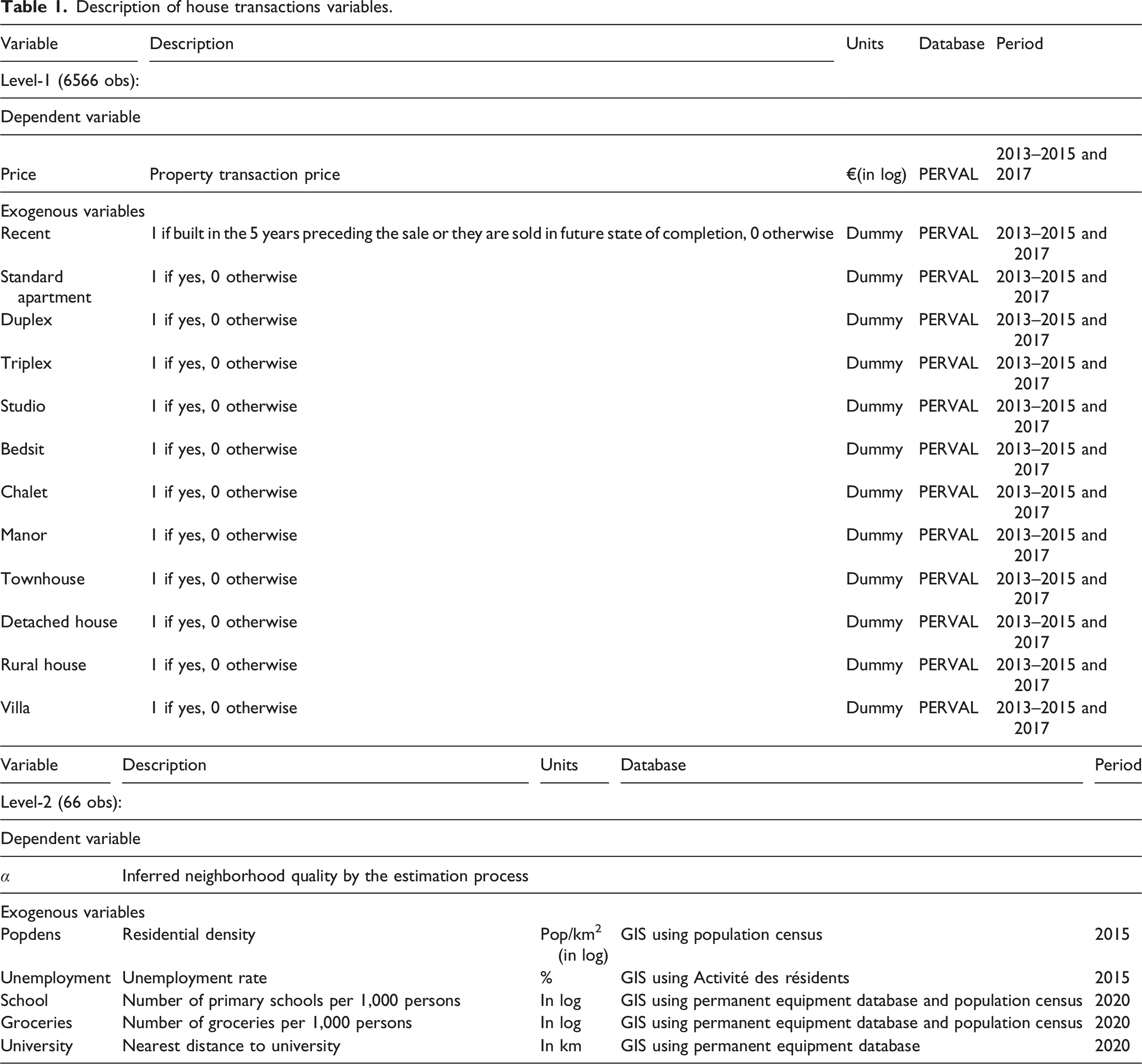
Description of house transactions variables.

Variable	Description	Units	Database	Period
Level-1 (6566 obs):		Units	Database	Period
Dependent variable
Price	Property transaction price	€(in log)	PERVAL	2013–2015 and 2017
Exogenous variables
Recent	1 if built in the 5 years preceding the sale or they are sold in future state of completion, 0 otherwise	Dummy	PERVAL	2013–2015 and 2017
Standard apartment	1 if yes, 0 otherwise	Dummy	PERVAL	2013–2015 and 2017
Duplex	1 if yes, 0 otherwise	Dummy	PERVAL	2013–2015 and 2017
Triplex	1 if yes, 0 otherwise	Dummy	PERVAL	2013–2015 and 2017
Studio	1 if yes, 0 otherwise	Dummy	PERVAL	2013–2015 and 2017
Bedsit	1 if yes, 0 otherwise	Dummy	PERVAL	2013–2015 and 2017
Chalet	1 if yes, 0 otherwise	Dummy	PERVAL	2013–2015 and 2017
Manor	1 if yes, 0 otherwise	Dummy	PERVAL	2013–2015 and 2017
Townhouse	1 if yes, 0 otherwise	Dummy	PERVAL	2013–2015 and 2017
Detached house	1 if yes, 0 otherwise	Dummy	PERVAL	2013–2015 and 2017
Rural house	1 if yes, 0 otherwise	Dummy	PERVAL	2013–2015 and 2017
Villa	1 if yes, 0 otherwise	Dummy	PERVAL	2013–2015 and 2017

Variable	Description	Units	Database	Period
Level-2 (66 obs):
Dependent variable
α	Inferred neighborhood quality by the estimation process
Exogenous variables
Popdens	Residential density	Pop/km² (in log)	GIS using population census	2015
Unemployment	Unemployment rate	%	GIS using Activité des résidents	2015
School	Number of primary schools per 1,000 persons	In log	GIS using permanent equipment database and population census	2020
Groceries	Number of groceries per 1,000 persons	In log	GIS using permanent equipment database and population census	2020
University	Nearest distance to university	In km	GIS using permanent equipment database	2020

Table 2.

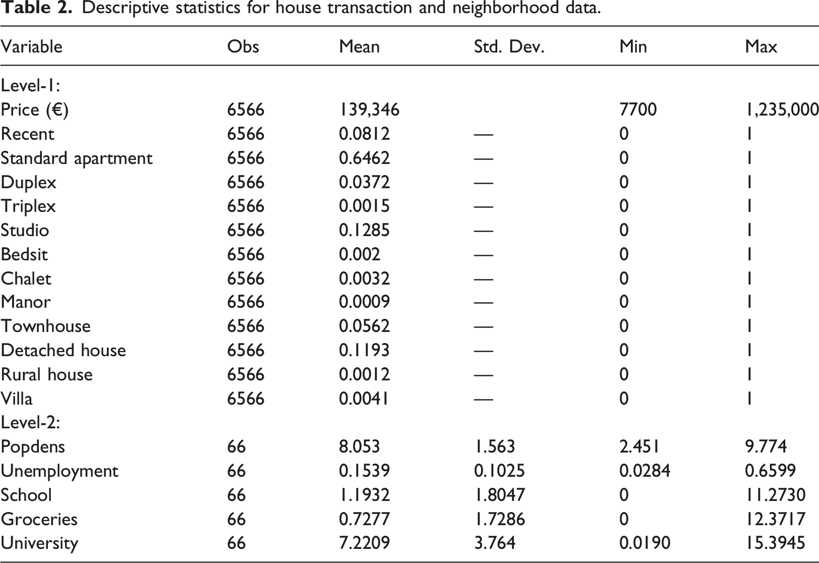
Descriptive statistics for house transaction and neighborhood data.

Variable	Obs	Mean	Std. Dev.	Min	Max
Level-1:
Price (€)	6566	139,346		7700	1,235,000
Recent	6566	0.0812	—	0	1
Standard apartment	6566	0.6462	—	0	1
Duplex	6566	0.0372	—	0	1
Triplex	6566	0.0015	—	0	1
Studio	6566	0.1285	—	0	1
Bedsit	6566	0.002	—	0	1
Chalet	6566	0.0032	—	0	1
Manor	6566	0.0009	—	0	1
Townhouse	6566	0.0562	—	0	1
Detached house	6566	0.1193	—	0	1
Rural house	6566	0.0012	—	0	1
Villa	6566	0.0041	—	0	1
Level-2:
Popdens	66	8.053	1.563	2.451	9.774
Unemployment	66	0.1539	0.1025	0.0284	0.6599
School	66	1.1932	1.8047	0	11.2730
Groceries	66	0.7277	1.7286	0	12.3717
University	66	7.2209	3.764	0.0190	15.3945

Figure 1.

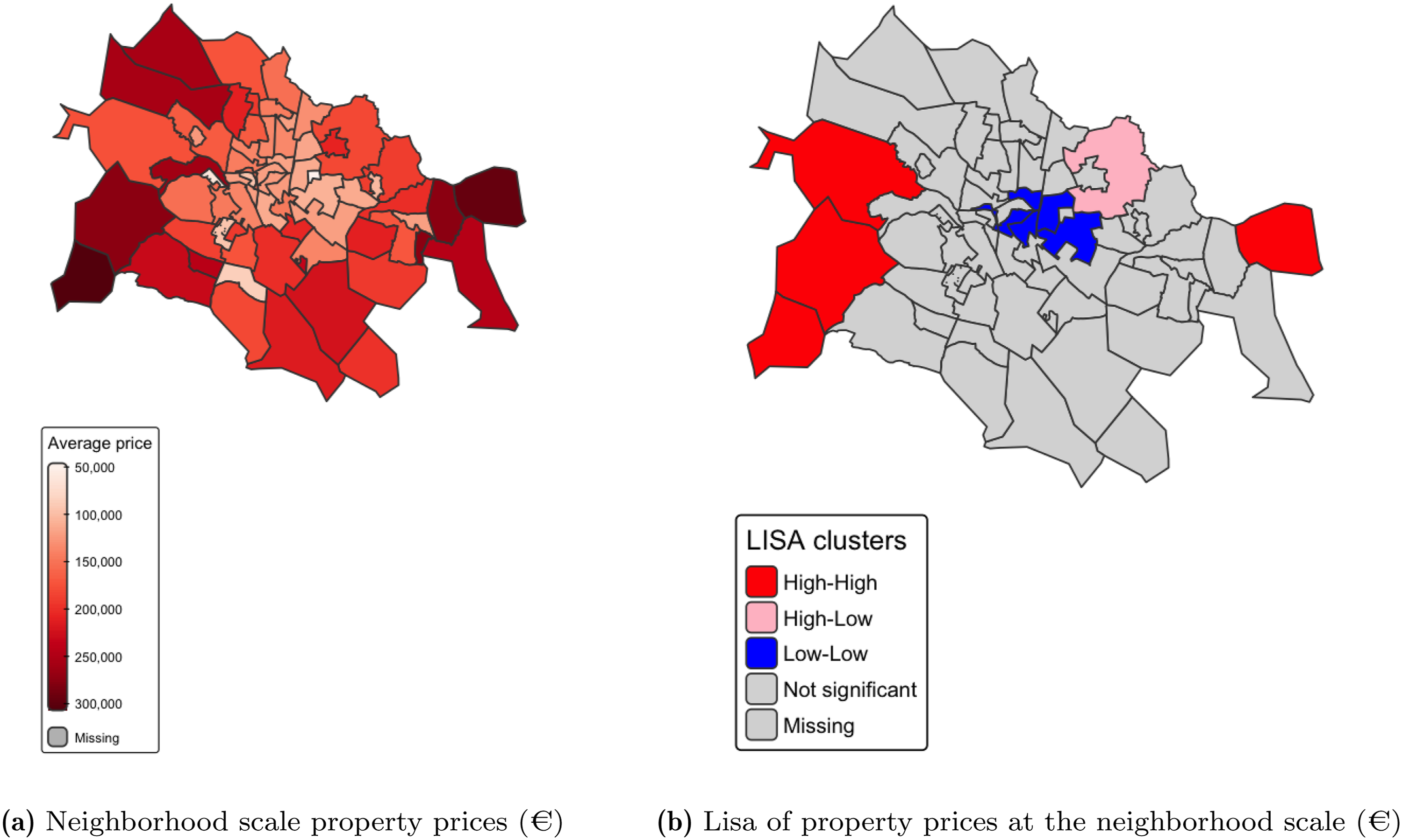
Neighborhood and LISA scale property prices.

The present study employs the PERVAL typology to delineate the various categories of real estate. A standard apartment is defined as a two-room apartment on one level, with the potential for a mezzanine. A duplex is defined as an apartment on two levels that is connected by internal or external stairs, while a studio is characterized as a one-room apartment. A triplex is distinguished by its tri-level configuration, it is interconnected by a series of staircases, some of which are internal and some of which are external, facilitating seamless and efficient movement between the various spaces. A chalet is defined as a wooden structure of any standard or quality. A manor is defined as an old stone house with a land area greater than 1000 m². A townhouse is a building with multiple floors, typically located on a street, avenue, or boulevard. These structures generally have a small land area, a cellar, an attic, a small garden, or a courtyard in the front, or a small garden in the back. A detached house is characterized by its lack of a specific architectural style and is typically constructed on a plot of land measuring approximately 600 m². These dwellings are often surrounded by a garden. A rural house is an older property, often situated in a rural area and typically having a lower price than other types of houses. Finally, a villa can be defined as a detached house characterized by its opulence, often featuring amenities such as swimming pools and tennis courts.

With respect to residential real estate transactions, the mean price of a dwelling is €139,346. The majority of the sample consists of standard apartments (65%), followed by studios (13%) and detached houses (12%). For further insights about the statistical distribution of housing prices and house types, readers can refer to Figure 2.

Figure 2.

Statistical distribution of house types and housing prices.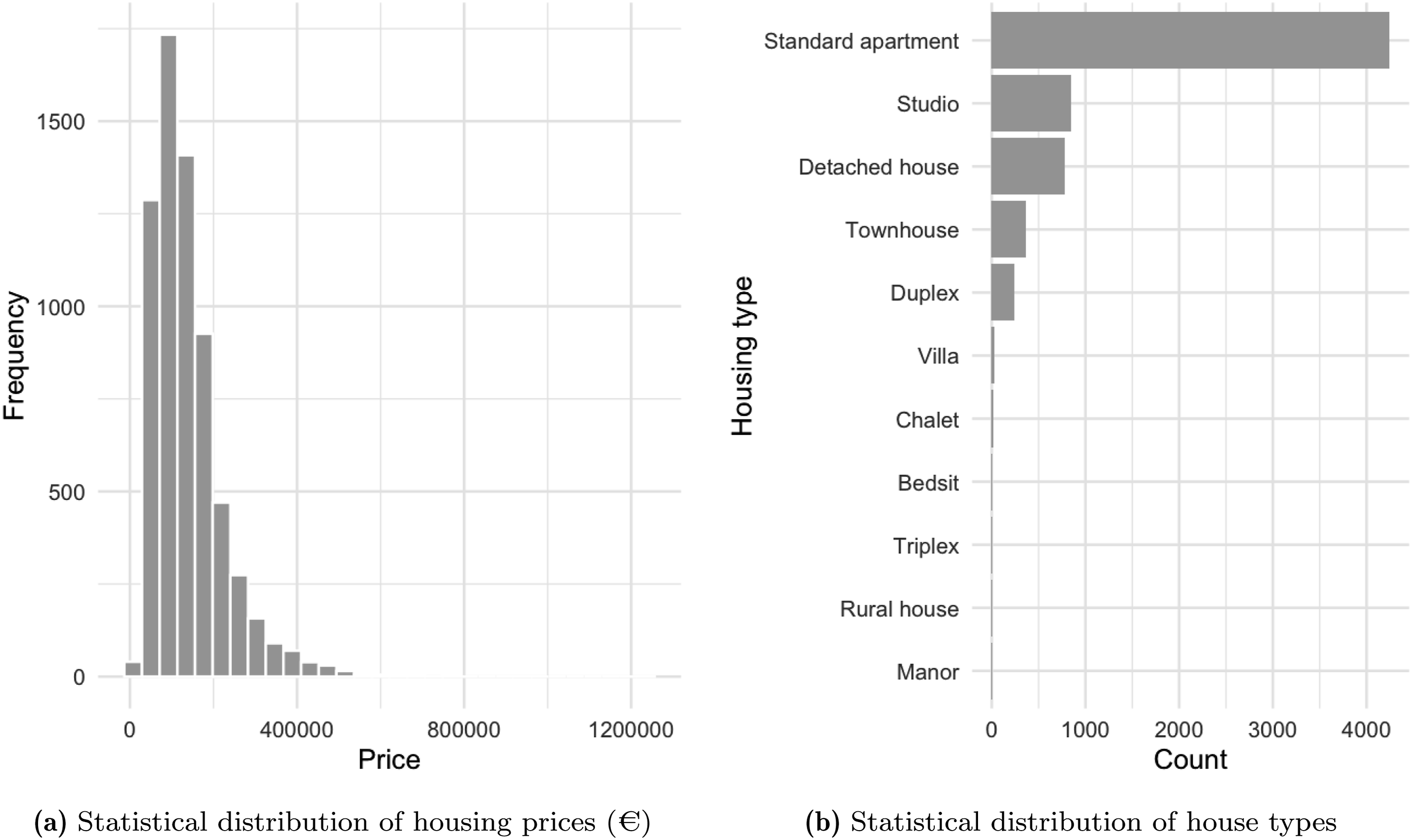

At the upper level, the groceries include hypermarkets, supermarkets and grocery stores. Descriptive statistics of neighborhoods highlight the differences among them. These statistics facilitate the identification of the “role” of each neighborhood in terms of the amenities it provides to its population.

Results and discussion

Lower-level effects: Housing characteristics

As demonstrated in Table 3, the posterior means and 90% credible intervals for the HSAR, HSLX, and HSDM models are reported. For ease of interpretation, exponentiated coefficients are discussed. According to the HSAR model, the average price of detached houses is 105.85%, 50.98%, and 293.93% higher than the prices of standard apartments, duplexes, and studios, respectively. A similar trend is evident in the market prices of manors and villas, which are, on average, 134.67% and 102.79% higher, respectively, than those of detached houses. Furthermore, the price of recent housing is 57.93% higher than that of older housing. More generally, these lower-level effects are strikingly similar across the three models. Furthermore, the credible intervals reveal no substantial differences between HSAR, HSDM, and HSLX. This finding indicates that the selection of upper-level spatial interaction structure exerts a relatively modest influence on the estimated effects of property-level characteristics.

Table 3.

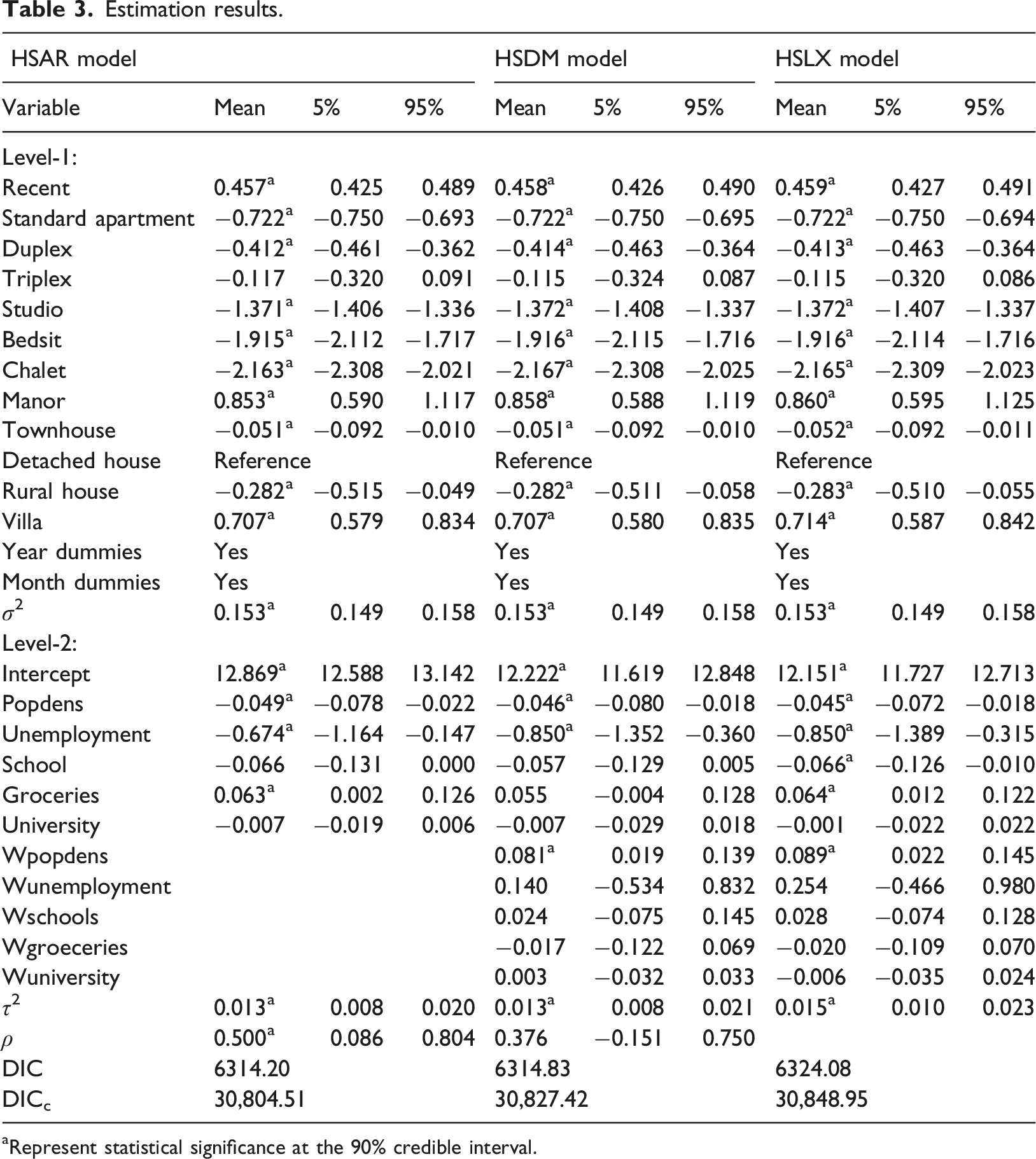
Estimation results.

HSAR model				HSDM model			HSLX model
Variable	Mean	5%	95%	Mean	5%	95%	Mean	5%	95%
Level-1:
Recent	0.457^a	0.425	0.489	0.458^a	0.426	0.490	0.459^a	0.427	0.491
Standard apartment	−0.722^a	−0.750	−0.693	−0.722^a	−0.750	−0.695	−0.722^a	−0.750	−0.694
Duplex	−0.412^a	−0.461	−0.362	−0.414^a	−0.463	−0.364	−0.413^a	−0.463	−0.364
Triplex	−0.117	−0.320	0.091	−0.115	−0.324	0.087	−0.115	−0.320	0.086
Studio	−1.371^a	−1.406	−1.336	−1.372^a	−1.408	−1.337	−1.372^a	−1.407	−1.337
Bedsit	−1.915^a	−2.112	−1.717	−1.916^a	−2.115	−1.716	−1.916^a	−2.114	−1.716
Chalet	−2.163^a	−2.308	−2.021	−2.167^a	−2.308	−2.025	−2.165^a	−2.309	−2.023
Manor	0.853^a	0.590	1.117	0.858^a	0.588	1.119	0.860^a	0.595	1.125
Townhouse	−0.051^a	−0.092	−0.010	−0.051^a	−0.092	−0.010	−0.052^a	−0.092	−0.011
Detached house	Reference			Reference			Reference
Rural house	−0.282^a	−0.515	−0.049	−0.282^a	−0.511	−0.058	−0.283^a	−0.510	−0.055
Villa	0.707^a	0.579	0.834	0.707^a	0.580	0.835	0.714^a	0.587	0.842
Year dummies	Yes			Yes			Yes
Month dummies	Yes			Yes			Yes
σ ²	0.153^a	0.149	0.158	0.153^a	0.149	0.158	0.153^a	0.149	0.158
Level-2:
Intercept	12.869^a	12.588	13.142	12.222^a	11.619	12.848	12.151^a	11.727	12.713
Popdens	−0.049^a	−0.078	−0.022	−0.046^a	−0.080	−0.018	−0.045^a	−0.072	−0.018
Unemployment	−0.674^a	−1.164	−0.147	−0.850^a	−1.352	−0.360	−0.850^a	−1.389	−0.315
School	−0.066	−0.131	0.000	−0.057	−0.129	0.005	−0.066^a	−0.126	−0.010
Groceries	0.063^a	0.002	0.126	0.055	−0.004	0.128	0.064^a	0.012	0.122
University	−0.007	−0.019	0.006	−0.007	−0.029	0.018	−0.001	−0.022	0.022
Wpopdens				0.081^a	0.019	0.139	0.089^a	0.022	0.145
Wunemployment				0.140	−0.534	0.832	0.254	−0.466	0.980
Wschools				0.024	−0.075	0.145	0.028	−0.074	0.128
Wgroeceries				−0.017	−0.122	0.069	−0.020	−0.109	0.070
Wuniversity				0.003	−0.032	0.033	−0.006	−0.035	0.024
τ ²	0.013^a	0.008	0.020	0.013^a	0.008	0.021	0.015^a	0.010	0.023
$ρ$	0.500^a	0.086	0.804	0.376	−0.151	0.750
DIC	6314.20			6314.83			6324.08
DIC_c	30,804.51			30,827.42			30,848.95

^aRepresent statistical significance at the 90% credible interval.

Upper-level covariates and neighborhood quality

Looking at the quality index (level-2), neighborhood qualities are statistically significant and generally decrease with the unemployment rate and population density. Conversely, the number of groceries per 1000 persons have a positive impact on neighborhood quality for HSAR and HSLX. Among the lagged covariates, only the spatial lag of population density is statistically significant in both the HSDM and HSLX models, whereas the lagged unemployment rate, the number of schools per 1000 persons, the number of groceries per 1000 persons and distance to university do not attain statistical significance at the 90% credible interval. Specifically, an increase of 100% in neighboring population density is associated with an increase of 0.089 units in the neighborhood quality, according to the spatial weighting matrix W for HSLX model. The findings of this study indicate that spatial dependence in housing prices functions predominantly through global endogenous interaction effects and, to a lesser extent, through local spillovers associated with neighboring population density.

The primary objective of our analysis is to elucidate the nature of spatial interaction at the neighborhood level. The posterior estimates indicate that the upper-level spatial autoregressive parameter, denoted by ρ, is positive and statistically significant in the HSAR model, suggesting the presence of global feedback effects in neighborhood-level housing prices. In contrast, the HSDM specification demonstrates that, while the posterior mean of ρ remains positive, its 90% credible interval includes zero. This finding indicates that the autoregressive effect is no longer statistically significant once spatially lagged covariates are introduced.

Global versus local and mixed spillovers at the upper-level

A comparison of model fit provides guidance for selecting the most appropriate specification. According to the complete DIC, the HSAR model yielded the lowest value (6314.20), closely followed by the HSDM model (6314.83), whereas the HSLX model displayed the highest value (6324.08).

While the complete DIC suggests a preference for models allowing for residual spatial dependence, it does not provide a definitive distinction between the global (HSAR) and mixed (HSDM) specifications. Indeed, the analysis becomes more definitive when the conditional DIC is considered, at which point the HSAR model (30,804.51) outperforms the HSDM model (30,827.42). This distinction is important because the conditional DIC reflects the fit of the first-level outcome equation, conditional on the estimated latent neighborhood effects. The lower conditional DIC of the HSAR model indicates that, once neighborhood-level heterogeneity is considered, the residual variation in housing prices is more efficiently captured by a global autoregressive process than by the incorporation of additional exogenous spatially lagged contextual variables.

Additionally, the interpretation of key parameters reinforces the preference for the HSAR specification. In the HSDM model, the posterior mean of the spatial autoregressive parameter ρ remains positive; however, its 90% credible interval includes zero. This finding suggests that the autoregressive effect becomes statistically insignificant once spatially lagged covariates are introduced. Consequently, the HSAR model provides a more parsimonious and statistically robust representation of spatial dependence. By prioritizing this parsimony, it can be concluded that the global autoregressive mechanism effectively captures the spatial dynamics of latent neighborhood quality. In contrast, the additional covariates in the HSDM model do not yield a superior representation of the observed data.

Robustness tests

To assess robustness, it is necessary to verify whether previous models were also estimated with different spatial weights matrices. Table 4 reports the DIC and DIC_c values obtained under alternative spatial weights matrices. A variety of spatial weights matrices were examined, including the following: W_eucl, an inverse Euclidean-based matrix between two contiguous neighborhoods, and

W_{k_{2}}

W_{k_{3}}

, and

W_{k_{4}}

, corresponding to the two-, three-, and four-nearest-neighbor matrices, respectively. In each case, row sums are equal to one.

Table 4.

Robustness results.

		HSAR	HSDM	HSLX
W _eucl	DIC	6317.58	6320.36	6329.45
W _eucl	DIC_c	30,819.75	30,817.71	30,853.77
$W_{k_{2}}$	DIC	6314.29	6314.19	6323.91
$W_{k_{2}}$	DIC_c	30,809.47	30,840.56	30,854.34
$W_{k_{3}}$	DIC	6317.53	6314.24	6325.52
$W_{k_{3}}$	DIC_c	30,800.78	30,836.26	30,853.94
$W_{k_{4}}$	DIC	6318.25	6315.91	6324.07
$W_{k_{4}}$	DIC_c	30,837.49	30,840.53	30,852.17

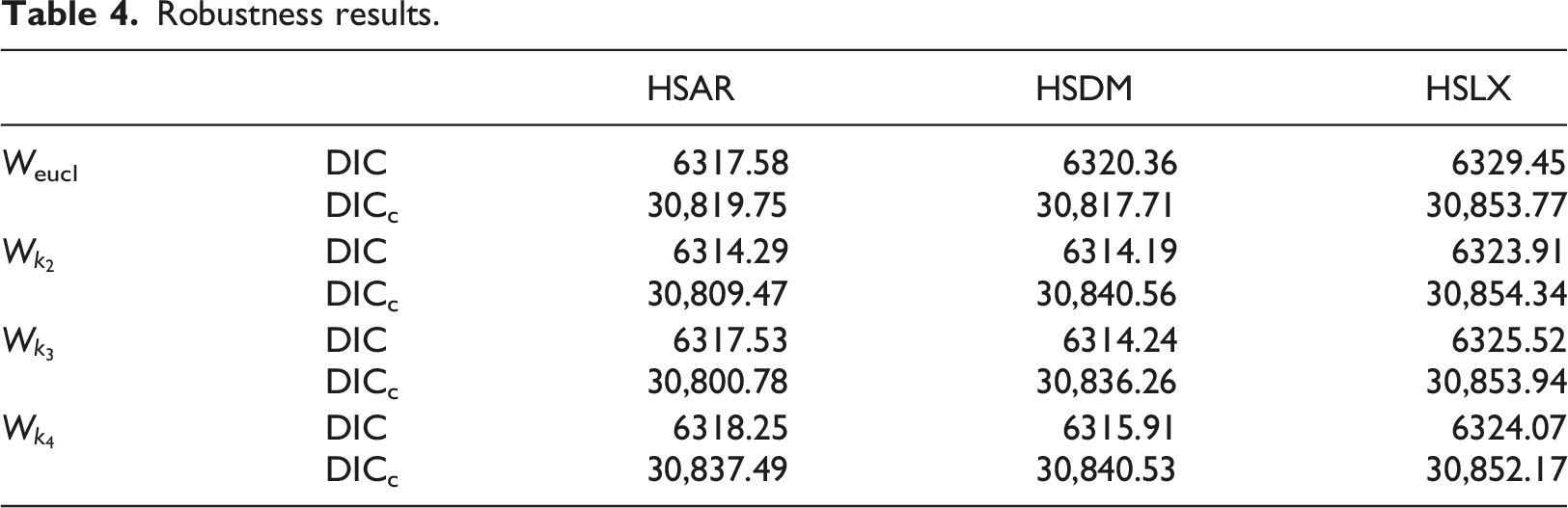
The robustness analysis, based on alternative spatial weights matrices, confirms the stability of the main conclusions. The conventional interpretation of DIC differences is as follows: values below 2 indicate negligible differences in fit, values between 2 and 7 suggest moderate evidence, and values above 10 indicate strong support for the model with the lower criterion value. According to the standard DIC, the HSLX model consistently provides the weakest fit across all spatial weighting matrices. For W_eucl, the HSAR model exhibits marginal superiority over HSDM, yet the discrepancy remains negligible. For $W_{k_{2}}$ , $W_{k_{3}}$ , and $W_{k_{4}}$ , the HSDM model attains the lowest DIC, but the difference with HSAR remains negligible. By contrast, the disparities between HSLX and the two alternative specifications are systematically more pronounced, suggesting that models incorporating endogenous spatial interaction provide a considerably superior fit.

A similar conclusion emerges from the conditional deviance information criterion (DIC_c), although the ranking between HSAR and HSDM differs somewhat. Under W_eucl, HSDM is marginally preferred, though the discrepancy with HSAR remains negligible. By contrast, under $W_{k_{2}}$ , $W_{k_{3}}$ , and $W_{k_{4}}$ , the HSAR model yields the lowest DIC_c values. In these cases, the relative superiority of HSAR over HSDM ranges from negligible to moderate, depending on the spatial weights matrix considered, while the gap relative to HSLX remains more pronounced. Overall, the robustness checks demonstrate that the substantive conclusions are not sensitive to the specification of the spatial weights matrix. The HSLX model is consistently dominated, whereas HSAR and HSDM systematically emerge as the preferred specifications. The comparison between these latter two models is more nuanced; however, the evidence from both DIC and DIC_c suggests that allowing for endogenous spatial dependence is essential for adequately capturing the spatial structure of housing prices. Moreover, a lower DIC_c for the HSAR model suggests that, conditional on the neighborhood-level structure, the HSAR specification offers a more appropriate representation of level-1 housing prices. In other words, once upper-level heterogeneity is taken into account, the residual spatial dependence in dwelling prices appears to be better captured by a global autoregressive mechanism than by exogenous spatial lags.

Conclusion

The objective of this paper is to make a methodological contribution to the field of hierarchical-spatial modeling for housing prices. For this purpose, it focuses on a yet often overlooked aspect: the nature of spatial interactions at higher levels of analysis. While the spatial dimension is readily identifiable at the level of individual dwellings, it becomes considerably more abstract and complex at the level of neighborhoods or cities, where spatial processes frequently serve as proxies for unobserved constructs such as neighborhood quality or the socio-economic environment. This inherent complexity renders the selection of spatial interaction at the upper level both theoretically and empirically critical.

To address this issue, the study proposed a comparative framework for evaluating different spatial interaction structures (endogenous, exogenous, and mixed) at the upper level of a hierarchical-spatial model. The aim of the study was to identify the most appropriate upper-level spatial interaction structure in a real-world context. To this end, the DIC was applied to a comprehensive dataset comprising 6566 dwelling transactions in Dijon Métropole, France, between 2013–2015 and 2017. The findings provide a clear empirical justification for the HSAR model. While the global and mixed structures appear competitive under the complete DIC, a more granular assessment, based on the conditional DIC and the credibility intervals of the spatial autoregressive parameter, favors the endogenous global process. This underscores the methodological value of not relying on a single criterion for model selection. By integrating fit diagnostics with parameter significance, it is established that the HSAR model offers a more parsimonious and statistically stable account of the latent spatial processes driving neighborhood housing prices.

Notwithstanding these contributions, the study has certain limitations that point toward avenues for future research. First, the analysis is restricted to a single metropolitan area, which may limit the generalizability of the findings to other urban contexts characterized by different spatial and socio-economic structures. Extending the comparative framework to multiple cities or regions would make it possible to assess whether the predominance of endogenous upper-level interactions is specific to Dijon Métropole or instead reflects a more general feature of urban housing markets. Second, although the robustness checks carried out with alternative spatial weights matrices confirm the stability of the main conclusions, the analysis remains limited to a restricted set of predetermined specifications. Future research could therefore investigate more flexible forms of spatial interaction, such as weights based on travel times, mobility flows, or other observed interaction data, and could also allow the spatial weights structure to vary across space. Finally, the present evaluation focuses primarily on in-sample model fit, as summarized by the DIC and the conditional DIC. Extending the analysis to include predictive accuracy measures, out-of-sample validation, or alternative loss functions would provide a more comprehensive assessment of model performance and would provide an additional robustness check.

Footnotes

Acknowledgment

The authors would like to thank the Editor and the anonymous reviewers for their valuable comments and constructive suggestions, which greatly improved the manuscript.

ORCID iD

Alper Acar

Ethical considerations

This study does not involve human participants, animals, or any data requiring ethical approval.

Consent for publication

During the preparation of this work the author used Deepl Write in order to improve readability and language. After using this tool/service, the author reviewed and edited the content as needed and take(s) full responsibility for the content of the publication.

Author contributions

All authors contributed to the conception and design of the study.

Funding

The authors received no financial support for the research, authorship, and/or publication of this article.

Declaration of conflicting interests

The authors declared no potential conflicts of interest with respect to the research, authorship, and/or publication of this article.

Data Availability Statement

Data are available on request from the authors.*

Notes

Author biographies

Alper Acar is an Assistant Professor in the Department of Economics at Galatasaray University, Turkey. His research focusses on spatial economics, spatial econometrics, and sports economics.

Catherine Baumont is a Full Professor of Economics at the Université de Bourgogne (Université Bourgogne-Franche-Comté, France) and a senior researcher at the Laboratoire d'Économie de Dijon (LEDi, UMR CNRS 6307). Her research interests focus primarily on urban and geographical economics, urban policies, and spatial econometrics.

References

Anselin

(1995) Local indicators of spatial association—lisa. Geographical Analysis 27(2): 93–115. https://doi.org/10.1111/j.1538-4632.1995.tb00338.x

Anselin

(2003) Spatial externalities, spatial multipliers, and spatial econometrics. International Regional Science Review 26(2): 153–166. https://doi.org/10.1177/0160017602250972

Anselin

(2022) Spatial econometrics. Handbook of Spatial Analysis in the Social Sciences. Edward Elgar Publishing, 101–122.

Banerjee

Carlin

Gelfand

(2014) Hierarchical Modeling and Analysis for Spatial Data. 2nd edition. Chapman and Hall/CRC.

Beron

Murdoch

Thayer

(1999) Hierarchical linear models with application to air pollution in the south coast air basin. American Journal of Agricultural Economics 81(5): 1123–1127. https://doi.org/10.2307/1244095

Cellmer

Kobylińska

Bełej

(2019) Application of hierarchical spatial autoregressive models to develop land value maps in urbanized areas. ISPRS International Journal of Geo-Information 8(4): 195. https://doi.org/10.3390/ijgi8040195

Chasco

Gallo

(2012) Hierarchy and spatial autocorrelation effects in hedonic models. Economics Bulletin 32(2): 1474–1480.

Chasco

Le Gallo

(2013) The impact of objective and subjective measures of air quality and noise on house prices: a multilevel approach for downtown Madrid. Economic Geography 89(2): 127–148. https://doi.org/10.1111/j.1944-8287.2012.01172.x

Corrado

Fingleton

(2012) Where is the economics in spatial econometrics? Journal of Regional Science 52(2): 210–239. https://doi.org/10.1111/j.1467-9787.2011.00726.x

10.

Dijon

(2023). Site cartographique du PLUi-HD de Dijon Métropole . https://api-carto.dijon.fr/plui/

11.

Djurdjevic

Eugster

Haase

(2008) Estimation of hedonic models using a multilevel approach: an application for the Swiss rental market. Swiss Journal of Economics and Statistics 144: 679–701. https://doi.org/10.1007/bf03399271

12.

Dong

Harris

Jones

, et al. (2015) Multilevel modelling with spatial interaction effects with application to an emerging land market in Beijing, China. PLoS One 10(6): e0130761. https://doi.org/10.1371/journal.pone.0130761

13.

Dong

Wolf

Alexiou

, et al. (2019) Inferring neighbourhood quality with property transaction records by using a locally adaptive spatial multi-level model. Computers, Environment and Urban Systems 73: 118–125. https://doi.org/10.1016/j.compenvurbsys.2018.09.003

14.

Gelfand

Banerjee

Sirmans

, et al. (2007) Multilevel modeling using spatial processes: application to the Singapore housing market. Computational Statistics & Data Analysis 51(7): 3567–3579. https://doi.org/10.1016/j.csda.2006.11.019

15.

Gelman

Hill

(2006) Data Analysis Using Regression and multilevel/hierarchical Models. Cambridge University Press.

16.

Gelman

Hwang

Vehtari

(2014) Understanding predictive information criteria for Bayesian models. Statistics and Computing 24(6): 997–1016. https://doi.org/10.1007/s11222-013-9416-2

17.

Glaesener

M-L

Caruso

(2015) Neighborhood green and services diversity effects on land prices: evidence from a multilevel hedonic analysis in Luxembourg. Landscape and Urban Planning 143: 100–111. https://doi.org/10.1016/j.landurbplan.2015.06.008

18.

Hall

Lacombe

Neto

, et al. (2022) Bayesian estimation of the hierarchical slx model with an application to housing markets. Journal of Economics and Finance 46(2): 360–373. https://doi.org/10.1007/s12197-021-09568-2

19.

Huang

Clark

(2002) Housing tenure choice in transitional urban China: a multilevel analysis. Urban Studies 39(1): 7–32. https://doi.org/10.1080/00420980220099041

20.

IGN. (2020). BD TOPO® – Département de la Côte-d'Or [Data set]. https://geoservices.ign.fr/bdtopo

21.

Insee . (2016, October 12). IRIS. Définitions, méthodes et qualité [Definitions, methods and quality]. https://www.insee.fr/fr/metadonnees/definition/c1523

22.

Insee . (2018a). Activité des résidents en 2015 – Recensement de la population – Base infracommunale (IRIS) [Activity of residents in 2015 – Population census – Infracommunal database (IRIS)] [Data set]. https://www.insee.fr/fr/statistiques/3627009

23.

Insee . (2018b). Population en 2015 – Recensement de la population – Base infracommunale (IRIS) [Population in 2015 – Population census – Infracommunal database (IRIS)] [Data set]. https://www.insee.fr/fr/statistiques/3627376

24.

Insee . (2021). Base permanente des équipements (BPE) en 2020 [Permanent database of facilities in 2020] [Data set]. https://www.insee.fr/fr/metadonnees/source/operation/s2027/bases-donnees-ligne

25.

Jones

(1991) Specifying and estimating multi-level models for geographical research. Transactions of the Institute of British Geographers 16: 148–159. https://doi.org/10.2307/622610

26.

Lesage

Pace

(2008) An introduction to spatial econometrics. Revue d’Économie Industrielle 123(123): 19–44. https://doi.org/10.4000/rei.3887

27.

Lesage

Pace

(2014) Interpreting spatial econometric models. In: Handbook of Regional Science. Springer, pp. 1535–1552.

28.

Manski

(2000) Economic analysis of social interactions. The Journal of Economic Perspectives 14(3): 115–136.

29.

Millar

(2009) Comparison of hierarchical Bayesian models for overdispersed count data using dic and Bayes’ factors. Biometrics 65(3): 962–969. https://doi.org/10.1111/j.1541-0420.2008.01162.x

30.

Ministère de la Transition écologique – SDES (2024). Base des permis de construire et autres autorisations d’urbanisme (Sitadel) en 2023 [Database of building permits and other urban planning authorizations (Sitadel) in 2023] [Data set]. https://www.data.gouv.fr/fr/datasets/base-des-permis-de-construire-et-autres-autorisations-durbanisme-sitadel/

31.

Moreira De Aguiar

Simões

Braz Golgher

(2014) Housing market analysis using a hierarchical–spatial approach: the case of Belo Horizonte, minas Gerais, Brazil. Regional Studies, Regional Science 1(1): 116–137. https://doi.org/10.1080/21681376.2014.934391

32.

Nordvik

Osland

Thorsen

, et al. (2019) Capitalization of neighbourhood diversity and segregation. Environment and Planning A: Economy and Space 51(8): 1775–1799. https://doi.org/10.1177/0308518x19861108

33.

Orford

(2000) Modelling spatial structures in local housing market dynamics: a multilevel perspective. Urban Studies 37(9): 1643–1671. https://doi.org/10.1080/00420980020080301

34.

Orford

(2002) Valuing locational externalities: a gis and multilevel modelling approach. Environment and Planning B: Planning and Design 29(1): 105–127. https://doi.org/10.1068/b2780

35.

Pérez-Molina

(2022) Exploring a multilevel approach with spatial effects to model housing price in San José, Costa Rica. Environment and Planning B: Urban Analytics and City Science 49(3): 987–1004. https://doi.org/10.1177/23998083211041122

36.

Piedra-Peña

Breuillé

Gallo

(2024) Municipal efficiency spillovers in France. The Annals of Regional Science 73(4): 2143.

37.

Spiegelhalter

Best

Carlin

, et al. (2002) Bayesian measures of model complexity and fit. Journal of the Royal Statistical Society Series B: Statistical Methodology 64(4): 583–639. https://doi.org/10.1111/1467-9868.00353

38.

Vega

Elhorst

(2013). On spatial econometric models, spillover effects, and w. In: 53rd ERSA Congress, Palermo, Italy, 27-31 August 2013, pp. 1–28.