Rethinking Type S and Type M Errors

Abstract

Gelman and Carlin introduced Type S (sign) and Type M (magnitude) errors to highlight the possibility that statistically significant results in published articles are misleading. Although these concepts have been proposed to be useful both when designing a study (prospective) and when evaluating results (retroactive), we argue that these statistics do not facilitate the proper design of studies or the meaningful interpretation of results. Type S errors are a response to the criticism of testing against a point null of exactly zero in contexts in which true zero effects are implausible. Testing against a minimum effect while controlling the Type 1 error rate provides a more coherent and practically useful alternative. Type M errors warn against effect-size inflation after selectively reporting significant results, but we argue that statistical indices such as the critical effect size or bias-adjusted effect size are preferable approaches. We do believe that Type S and Type M errors can be valuable in statistics education, in which the principles of error control are explained, and in the discussion section of studies that fail to follow good research practices. Overall, we argue that their use cases are more limited than is currently recognized and that alternative solutions deserve greater attention.

Keywords

Type M error Type S error error control hypothesis testing bias correction open data

Neyman-Pearson hypothesis testing is a widespread approach to statistical inferences in the social sciences. Power analyses have increased to 30% across all articles that conducted a quantitative primary analysis across psychological disciplines, and there has been an adoption of 46.7% in experimental psychology (Vankelecom et al., 2025). Using a prespecified alpha level is increasingly common with the adoption of preregistration of statistical analysis plans (J. Ferguson et al., 2023). As a consequence of its popularity, Neyman-Pearson hypothesis testing is commonly criticized, and critics regularly propose alternative statistical procedures to interpret results. One criticism of null hypothesis tests is that the null hypothesis is never true (Cohen, 1994). Gelman and Tuerlinckx (2000) argued that because it seems unlikely that effect sizes are ever exactly zero for continuous data, it is uninteresting to control the probability of a Type 1 error. After all, if the null is never true, researchers do not need to worry about incorrectly claiming there is an effect when there is no effect. They proposed to compute the Type S error, or “sign error,” which quantifies the long-run frequency that a significant effect in the opposite direction of the true effect size is observed. The probability of a Type S error is at most 2.5% (the probability of an extreme result in the tail of the distribution opposite to the true effect) and, in practice, is often trivially small. They argued that Type S error rates are “the relevant error rate for statistical analyses in the social and behavioral sciences” (p. 388). Gelman and Tuerlinckx also proposed to report the Type M error, which quantifies the extent to which effect-size estimates are overestimated because of selection bias. For example, a Type M error of 2 indicates that the absolute average effect-size estimates after all nonsignificant studies are removed will be twice as large as the true effect size. Gelman and Carlin (2014) suggested that Type M errors are useful to understand that significant effect sizes from underpowered studies are almost certain to be a huge overestimate of the true effect. Gelman and Carlin wrote that problems with Type S errors become a concern “when power is less than 0.1” and that Type M errors become a concern “when power is less than 0.5” (p. 644).

Before criticizing the proposed use of Type S and Type M errors, it is important to acknowledge several points of agreement. First, we agree with Gelman and Tuerlinckx (2000) that it is uninteresting to test against a null hypothesis of no effect when it is highly unlikely that the true effect size is zero. However, we believe this problem should be addressed by performing a minimal-effect test for superiority against a range of values that is considered practically equivalent to zero. Such tests against a non-nil-null hypothesis have been suggested for more than half a century (Hodges & Lehmann, 1954; Lakens, 2021; Nunnally, 1960; Serlin & Lapsley, 1985). We also agree with Gelman and Carlin (2014) that performing an a priori power analysis based on estimates of a previous study or an expected effect size is not best practice and leads to bias (Albers & Lakens, 2018). However, we see no problem with what is currently considered best practice—performing an a priori power analysis based on a smallest effect size of interest (SESOI)—just because the true effect size might be smaller than the SESOI. Trivially small effect sizes are scientifically uninteresting, and researchers should not be interested in detecting effects that are too small to matter (Lakens, 2022).

Third, we agree that publication bias is a systemic problem in the social sciences that leads to inflated effect sizes in the scientific literature. In situations in which no assumed plausible effect size under the alternative hypothesis is available, reporting the critical effect size (e.g., Perugini et al., 2025) may offer a more informative perspective than computing a Type M error, which relies on such an assumption. Finally, we recognize that it is valuable to retrospectively evaluate how informative studies in a literature are, especially in fields in which good research practices are uncommon. However, we believe a sensitivity power analysis combined with bias-correction methods, such as p-uniform (Van Aert & Van Assen, 2018) or a maximum likelihood estimate for a truncated distribution (Anderson & Maxwell, 2017; Taylor & Muller, 1996), are more insightful. Finally, E. Toffalini and G. Altoè have coauthored scientific articles promoting Type S and Type M errors (Altoè et al., 2020; Bertoldo et al., 2022) and cocreated the R package PRDA, which computes Type S and Type M errors for different designs (Callegher et al., 2021). They were invited to coauthor this article to guarantee fair and nuanced arguments by incorporating internal criticism into this project (Lakens, 2020). E. Toffalini and G. Altoè found the discussions that shaped the article intellectually rewarding, and the discussions confirmed the view—also expressed in the article—that Type S and Type M errors, although not without limitations, can serve as useful concepts to foster critical reflection and statistical awareness. Like many tools in scientific practice, their usefulness does not lie solely in their technical properties but in researchers’ ability to understand their logic, reflect on their limitations, and apply them thoughtfully.

Type 1, Type 2, Type 3, and Type S errors

Type 1 errors occur when the null hypothesis is true but a statistically significant result is observed. The null hypothesis in a two-sided test is that the population effect size is 0. The alternative hypothesis is that there is an effect—in either the positive or negative direction. After observing a statistically significant result, the correct claim is that the null hypothesis can be rejected and that one can act—with a maximum error rate of α—as if there is a nonzero effect. Because no directional claims are made in a correctly performed two-sided null-hypothesis test, sign errors are impossible in two-sided hypothesis tests. There are other tests in which sign errors cannot occur, such as an omnibus F test used to detect differences between groups, because the F distribution is based on squared deviations and has only positive values.

Researchers sometimes incorrectly make a directional claim after a two-sided test, which can lead to what Kaiser (1960) referred to as an “error of the third kind.” An error of the third kind occurs when H0 is false, a statistically significant effect is observed in the opposite direction of the true effect, and researchers make a directional claim. The correct way to make directional claims is to perform a one-sided test. If researchers want to make a claim about an effect in the positive or negative direction, they should follow Kaiser’s proposal to perform two one-sided null-hypothesis tests, one in the positive direction and one in the negative direction, each at α / 2 (see also Leventhal & Huynh, 1996). This would not change the conclusions researchers draw in practice compared with the current widespread use of two-sided tests, but it would make these conclusions logically coherent.

According to Gelman and Tuerlinckx (2000), effects are never exactly zero. This led them to argue that it is uninteresting to perform a null-hypothesis test or to control the Type 1 error rate. They proposed to remove effects of 0 from the possible effect sizes that can be observed. This creates a situation in which all effects are true effects in either the positive or the negative direction. A statistical test now has two possible results: Effects in the opposite direction as the true effect size are correctly rejected, or effects in the true direction are incorrectly rejected—a Type S error. Type S errors can be computed for any test that makes claims based on a threshold (for closed-form formula, see Lu et al., 2019), but in this article, we focus on frequentist hypothesis tests. We set the alpha level for the test to .05 in all examples below.

If one believes effect sizes of 0 do not exist, it is no longer possible to perform a two-sided nil-null-hypothesis test. Gelman and Tuerlinckx (2000) instead recommended performing two simultaneous one-sided tests: one test in the positive direction and one test in the negative direction. To understand Type S errors, it is useful to consider the most extreme scenario in which the effect size is not zero. If there is an infinitesimally small positive effect, the statistical power of the test is practically indistinguishable from the alpha level of .05. Effects will be rejected in the positive direction with a probability of .025 in the long run (correct rejections), and effects will be rejected in the negative direction with a probability of .025 in the long run (Type S errors). The only difference between a Type S error and a Type 1 error in this scenario is that Gelman and Tuerlinckx removed the value of 0 from the distribution of possible effect sizes. A Type 1 error consists of all significant test results for values ≤ 0, and a Type S error consists of all significant test values < 0. Because any point in a continuous distribution has 0 probability, excluding the value of 0 will not change the long-run probabilities. The difference between a Type 1 error and Type S error in this extreme scenario is purely conceptual.

When two one-sided tests are performed and the null is false, the Type S error rate is at most α / 2. Gelman and Turelinckx (2000) preferred to express the Type S error rate as a proportion of the significant results and “believe that this conditional probability is the appropriate error rate to consider, since our primary concern is to understand the frequency properties of claims with confidence” (p. 380). In the infinitesimal-effect case, the statistical power of the test is .05, and the Type S error is .025, so the rate of Type S errors as a proportion of significant results is .025 / .05 = .5. In the extreme case in which power is as low as the alpha level, 50% of significant results are sign errors.

This conditional probability is similar to the false-discovery rate, which is the expected proportion of false positives among all positive findings. Just as Type 1 errors occur only when the null hypothesis is true, the false-discovery rate occurs only when the null hypothesis is true. But once again, removing the value of 0, which itself has 0 probability, does not change the long-run false-discovery rate. If researchers believe the null is true, a Type 1 error (a rejection of positive effects when there is a positive effect) will be observed with a probability of .025, and a correct rejection (a rejection of negative effects when there is a positive effect) will occur with a probability of .025. From all positive findings (.025 false positives + .025 true positives = .05 positive test results), 50% are false positives. Therefore, the false-discovery rate is 50% in the two one-sided-testing procedures. The maximum conditional Type S probability is identical to the false-discovery rate with the conceptual difference that it excludes the value of 0 from the hypothesized values. Type S errors differ from Type 1 errors and false-discovery rates in that they can be computed for a range of assumed true effect sizes. But because Type 1 error rates are already small, Type S probabilities quickly become even smaller, and because the true effect size is unknown, the added value of presenting a range of Type S error rates remains unclear.

Should Effects of 0 Be Considered Impossible?

Note that it is somewhat peculiar to completely exclude the possibility that effect sizes of 0 exist in a hypothesis test. After all, one could just as easily argue that in continuous data, no true effect size is exactly 0.5, but no one would propose to remove 0.5 from the space of hypothesized values. Researchers have also disagreed with the idea that effect sizes are never 0; Krueger and Heck (2019) stated that “for many questions humans ask of nature, the null (or any particular tested hypothesis) may in fact be true” (p. 125). Frick (1995) concluded that “for some experiments, the null hypothesis is possible.” And Hagen (1997) drove home the criticism even more forcefully:

If, as some have claimed, the null hypothesis is always false, we would be foolish, indeed, to spend time conducting statistical tests that can only tell us what we already know. But we need not feel foolish. As far as I can tell, the claim has never been sustained by either statistical or logical arguments. (p. 21)

Neither side can provide empirical support for or against the hypothesis that the null hypothesis is never true because one cannot measure the entire population for all effects scientists want to study. The claim that the null is never true is scientifically unfalsifiable.

It seems difficult to justify why one would believe the null is never true when there is no doubt that an effect size of 1 × 10⁻³² can be true. Instead of discussing which effect sizes can be true, a more sensible concern is the idea that all variables are connected through theoretically uninteresting causal structures that result in nonzero correlations between variables (especially in observational studies). In psychology, this idea is referred to as the “crud factor” (Meehl, 1990; Orben & Lakens, 2020). The crud factor has been one argument to move beyond null-hypothesis significance tests and instead test against a range of theoretically or practically uninteresting effect sizes around zero by performing a minimum-effect test, or a test for superiority (Lakens et al., 2018).

Instead of performing a test that rejects effect sizes of 0, researchers can specify an SESOI and test whether they can statistically reject all effects that are deemed too small to matter. Minimum-effect tests resolve most of the problems researchers have with nil-null-hypothesis significance testing (Lakens, 2021), including the concern that the null is never true. If researchers do not believe it is scientifically interesting to reject effects of exactly 0, they can test whether effects in a range around 0 can be rejected. For example, C. J. Ferguson and Heene (2021) empirically showed that correlational effects in aggression research are unlikely to ever be exactly 0 and established a correlation of r = .1 as a lower bound for hypothesis tests in this research field. A directional minimum-effect test against r ≤ .1 is rejected if the lower bound of the 90% confidence interval around the observed correlation is larger than .1 (Lakens et al., 2018). Minimum-effect tests are a better solution than arbitrarily excluding a point value of 0 from the range of effects that are considered possible. If minimum-effect tests are adopted, the idea of a Type S error is no longer needed because it is equivalent to a Type 1 error for one-sided tests against a non-nil-null hypothesis.

Should Researchers Report Type S Errors in Scientific Articles?

Whereas Gelman and Tuerlinckx (2000) discussed only the relevance of Type S errors relative to Type 1 errors, Gelman and Carlin (2014) took an additional step and suggested that it is useful to compute and report Type S error rates for specific studies. To compute a Type S error, researchers need to specify what they believe is the true effect size. Gelman and Carlin suggested using a literature review or other available data. They provided an example in which the original author observed an effect of 8 percentage points. Gelman and Carlin did not believe this finding could be correct and retrospectively computed the Type S error based on effect sizes they believed were more likely to be true: 0.1, 0.3, and 1 percentage point. When they computed the Type S error for the much smaller effects they deemed plausible, the probability of a sign error can be quite large as long as the statistical power is low.

Is it useful to compute and report Type S errors in this way? One problem with retrospective design analysis is that if skeptics want to argue that an effect size is unreliable, a retrospective design analysis will practically never prove them wrong. For any effect for which a skeptical reader feels the need to question the scientific claim by performing a retrospective design analysis, there will be substantial uncertainty about the true effect size. In these cases, the literature (or any other external data) will rarely—if ever—provide strong constraints on how small effect sizes can plausibly be. This means a skeptical reader can always find reasons to perform a retrospective design analysis for very small effect sizes, which makes it easy to claim that there is a high probability of a sign error. If the skeptics are wrong, a retrospective design analysis would practically never tell them they are wrong, and claims about high Type S error rates are therefore rarely severely tested.

To conclude this section, we have strong conceptual issues with Type S errors (removing 0 from the range of possible distributions is difficult to justify, and the long-run probability of Type S errors is identical to the well-established Type 1 error rate and false-discovery rate) and practical concerns (the test can too easily lead to a foregone conclusion). Type S errors mainly point out how uninformative studies with low statistical power are, and a null-hypothesis test might not be an interesting question to ask. If researchers want to address these concerns, a better solution is to specify a non-nil-null hypothesis (e.g., considering all effects between −0.1 and 0.1 as practically equivalent to 0) and perform an a priori power analysis for the SESOI. After the data are in, the Type S error is at most 2.5%, as is the Type 1 error. Researchers should always make a claim while acknowledging the maximum possible Type 1 error rate (e.g., 2.5% in a one-sided test with an alpha level of .025) and that any quantification of how much lower the Type S error might be, depending on weakly informed guesses of the true effect size, comes with great uncertainty.

Gelman and Carlin (2014) argued that a retrospective design analysis can reveal that “a study was too small to be informative.” But this seems misguided. If a significant effect was observed in a well-performed test, one can reject the null with a maximum Type 1 error rate of 2.5%, which is small enough to take the result seriously. The study might have had very low power to detect an effect, but if it happened to detect an effect with the desired maximum Type 1 error rate, the fact that the study had a low probability to yield an informative outcome a priori no longer matters. The observed effect size might be measured inaccurately and inflated because of selection bias (see Type M errors below), but a researcher can claim that the probability that random noise is mistaken for a true effect is very small.

The Type S error rate will raise a red flag only for studies with incredibly low statistical power. When the Type S error is high, the design is uninformative (e.g., when the Type S error rate is at its maximum of 2.5%, the study has a statistical power of merely 5%). But when the Type S error is low, the design is often still uninformative. The Type S error drops to negligible levels when the statistical power of the test is still unacceptably low. For example, Simonsohn (2015) considered a test with less than 33% power severely underpowered, but with 33% power, the probability that a significant result is in the wrong direction is only 0.1%.

Effect-Size Inflation and Type M Errors

Lane and Dunlap (1978) examined the impact of selection bias on the inflation of effect-size estimates. When only statistically significant results are shared, the effect-size estimate based on these studies is inflated because smaller nonsignificant effects are removed from the scientific literature. In general, how much effect sizes are inflated in the presence of selection bias is a function of the power of the test. The lower the statistical power is—for example, because population effect sizes or sample sizes are smaller—the more significant effect sizes will be inflated. Figure 1 shows the expected effect-size distribution for an alternative hypothesis with a true effect size of Cohen’s d of 0.5. With a sample size of 40 participants in each group, a two-sided independent t test will yield a statistically significant result if the observed effect size is larger than d = 0.445. If there is extreme selection bias for statistically significant results, the scientific literature would consist of effect sizes to the right of d = 0.445. Instead of having access to the full distribution of expected effects, the literature will represent a truncated distribution, in which all values smaller than 0.445 are removed from the distribution of expected effect sizes.

Fig. 1.

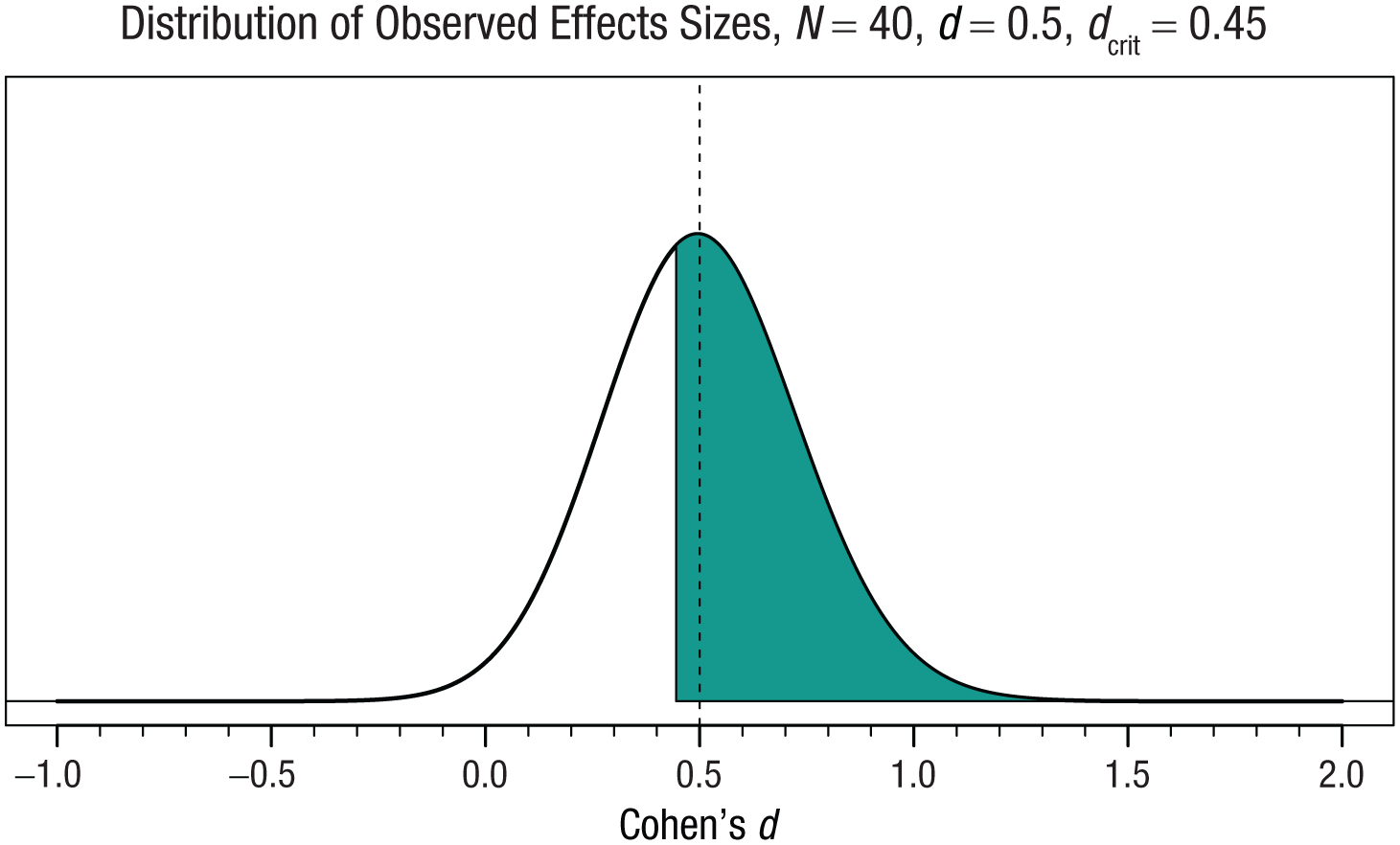
Expected effect-size distribution under the alternative hypothesis, assuming a true effect size of 0.5 (dashed central line). With a sample size of 40 participants per group, a two-sided independent t test yields a statistically significant result when the observed effect size exceeds d = 0.45. The shaded area represents the subset of effect sizes published under selection bias.

This type of bias has been discussed extensively in the literature (Anderson & Maxwell, 2017; Begg & Mazumdar, 1994; Hedges, 1984). Both Hedges (1984) and Taylor and Muller (1996) developed a statistical model that computes bias-adjusted effect-size estimates when estimators are selected from a “censored” or “truncated” distribution. This method creates a model of what the full distribution would have looked like and estimates the effect size if there were no selection bias. Anderson et al. (2017) applied this method to compute an adjusted estimate of the noncentrality parameter and used it to show how a priori power analyses can be adjusted for selection bias.

Gelman and Carlin (2014) proposed another approach to increase awareness of effect-size inflation because of selection bias. They computed a ratio between the average absolute effect-size estimates from statistically significant effects and the assumed true effect size, which they referred to as a “Type M” (magnitude) error. Because Type M errors do not quantify error rates (i.e., the probability of an incorrect claim) but rather, the bias in an estimator, we prefer Gelman and Carlin’s alternative term for Type M errors: the “exaggeration ratio.” The exaggeration ratio is a function of the statistical power of a test. When power is close to 100%, all tests of true effects will be significant, no effect sizes are removed because of selection bias, and the exaggeration ratio will be 1, indicating that the design will in the long run yield unbiased effect-size estimates. Because power is practically always less than 100%, the exaggeration ratio will typically be larger than 1, indicating that effect sizes selected for statistical significance will be inflated. Altoè et al. (2020) noted that when power reaches at least 80%, the average overestimation of the effect size tends to be just above 10%, which they considered practically negligible. Thus, one may see the exaggeration ratio as a complementary perspective on the information conveyed by statistical power, shifting the focus from hypothesis testing to effect-size estimation.

The exaggeration ratio is computed based on properties of the design of the study and the assumed true effect size. The design (e.g., the sample size, type of test, and the alpha level) determines the critical effect size, or the smallest effect size that can be statistically significant. The assumed true effect size determines the extent to which effect sizes that are selected for significance will be inflated. The smaller the assumed effect size is, the larger the exaggeration ratio is. The exaggeration ratio (Gelman & Carlin, 2014) is not intended to correct individual effect sizes. If the average absolute unbiased effect-size estimate is 0.5 and the average biased effect-size estimate is 1, the estimated effect is on average 2 times larger than the true effect size. But this exaggeration ratio of 2 applies to the average effect-size estimate and not to any individual effect size. It is not correct to simply divide each observed effect-size estimate by the exaggeration ratio and treat it as a bias-adjusted effect-size estimate.

Despite the fact that Gelman and Carlin (2014) never intended the exaggeration ratio to be used to adjust individual effect sizes, researchers have misused Type M errors for this purpose. In the following example, Shem-Tov et al. (2024) noted that the Type M error rate quantifies an average inflation but still misused it to adjust the observed effect size:

Following the procedure proposed by Gelman and Carlin (2014), we estimate an average potential exaggeration ratio of 1.2 in the effect of enrollment to Make-it-Right (MIR) on rearrests within one and four years. In other words, on average, our estimates might indicate that the impact of enrollment to MIR causes a reduction of 23.4 percentage points while the true effect is a reduction of 19.5 percentage points. (Online Supplement, p. 1)

Likewise, Gajendran et al. (2022) wrote, “The modest Type M exaggeration ratio of 1.27 indicates the possibility that the communication medium effect is overestimated by a factor of 1.27, which is inconsistent with the effect being an unlikely result.” However, the average inflation is not the same as the inflation in any individual study, and the inflation might be much larger or smaller for this specific study.

There are statistical approaches that perform a bias adjustment on a single biased effect size (Hedges, 1984; Taylor & Muller, 1996). The approaches developed by Hedges (1984) and Taylor and Muller (1996) attempt to adjust effect-size estimates for selection bias by taking the observed effect size and based on a model for selection bias, return the maximum likelihood estimate for the effect size after correcting for bias. Anderson et al. (2017) implemented this bias-correction method in the BUCSS R package to provide a priori power analyses for bias-adjusted effect-size estimates. The p-uniform technique developed by Van Assen et al. (2015) uses a similar model for selection bias as Hedges and will estimate an unbiased effect-size estimate for a single study. Although this has not been pointed out explicitly in the literature, the corrections based on BUCSS and p-uniform are practically identical, and therefore, we discuss adjustments using only p-uniform.

To illustrate why this misuse of Type M errors fails to adequately adjust observed effect sizes for bias, we simulated 100,000 independent t tests with a true effect size of d = 0.5, 40 observations per group, equal variances, and an alpha level of .05 and removed all nonsignificant test results to introduce selection bias. The distribution in Figure 2 (left) shows the effect-size distribution of observed effect sizes when only statistically significant results are available (green) and the missing nonsignificant results (gray). Given the sample size, only effects larger than d = 0.445 will be statistically significant, and all effects smaller than d = 0.445 are missing from the truncated distribution. Figure 2 (middle) shows the distribution if individual effect sizes are adjusted by the exaggeration ratio. Large observed effects are adjusted downward a lot, but smaller observed effect sizes are not sufficiently adjusted downward. Figure 2 (right) shows computed adjusted effect sizes based on p-uniform. When applying p-uniform in its intended context of meta-analyses, users are recommended to replace negative estimates by 0 (Van Aert et al., 2019). This solution is less ideal when analyzing single studies because too many estimates will be set to 0, which negatively biases the estimate. Instead, we follow the recommendation by Anderson et al. (2017) and remove negative estimates in Figure 2. The bias-adjusted effect-size estimates from p-uniform do not perfectly match the unbiased distribution but provide estimates that are on average much closer to the true effect size. This simulation shows that although the exaggeration ratio can be used to educate researchers about the risk of inflation, it cannot be used to adjust individual effect sizes for selection bias, as some researchers in the literature have done.

Fig. 2.

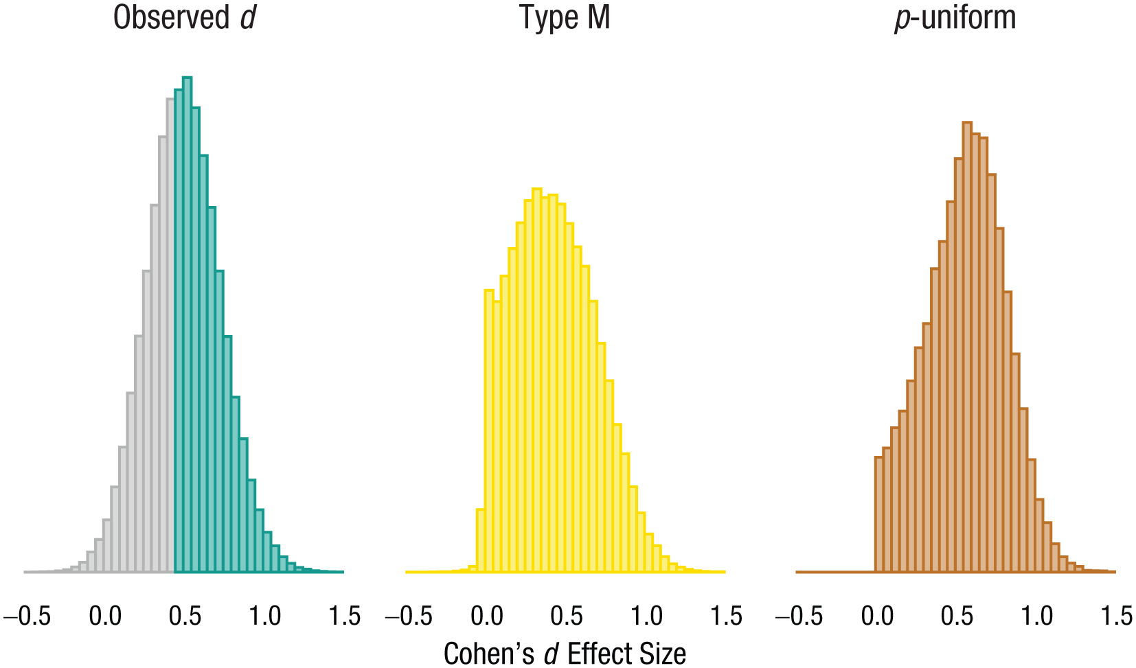
Comparison of the observed effect sizes (green; gray area illustrates missing nonsignificant values) and bias-adjusted effect sizes using two methods: the Type M exaggeration ratio (yellow) and p-uniform (brown).

All approaches to adjust effect sizes for bias because of selective reporting rely on overly simplistic models of bias and depend on strong assumptions that are almost always violated, and for these reasons, bias-adjusted effect-size estimates rarely correspond to empirically observed effect sizes from unbiased studies (Kvarven et al., 2020). These problems are even more pronounced when a bias-adjusted effect-size estimate is calculated for a single effect size because of the large variability in a single effect-size estimate. Bias-adjusted effect-size estimates that differ substantially from the unadjusted effect size should not be regarded as the true unbiased effect size but as a strong motivation to perform an unbiased replication study.

Reporting the critical effect size might provide an alternative approach to increase awareness about effect-size inflation because of selection bias. Reporting critical effect sizes has benefits over reporting the exaggeration ratio (Perugini et al., 2025). The critical effect size is the smallest effect size that could reach statistical significance. Similar to the exaggeration ratio, it is computed based on the study design. The critical effect size highlights how selecting statistically significant results will remove all effect sizes smaller than the critical effect size. Reporting a critical effect size does not provide a single numerical estimate of how much the effect is inflated, which prevents the misinterpretation of the exaggeration ratio that we observed. Critical effect sizes also warn against interpreting nonsignificant results as the absence of an effect because they highlight that there is a range of true effects below the critical effect size that would lead to nonsignificant results. And finally, critical effect sizes are also useful in studies with very high statistical power. In such studies, the exaggeration ratio would be negligible, but the critical effect size would increase awareness that even trivially small effects will be statistically significant, which will make researchers reflect on which effects are large enough to be meaningful.

The Use of Type S and Type M Errors in an “Imperfect” Science

Although Type S and Type M errors might not be particularly informative to report in a results section, given the more informative alternatives (i.e., minimum-effect tests and bias-corrected effect-size estimates), they may still be valuable as a tool to reflect on the problems that emerge when studies are underpowered and/or selectively reported. Because of resource constraints, researchers may sometimes perform studies with very low power for the main effect of interest. Consider a PhD student who can at most collect 20 participants per group for an independent two-sided t test and expects a true effect size of d = 0.4. An a priori power analysis reveals that the statistical power is a mere 23%. With such a high probability of uninformative results, one might argue that the study should not be performed. However, the study is part of a grant proposal that funds the research of the PhD student, and the student’s supervisor wants to complete the promised data collection regardless of the low statistical power. Under these suboptimal conditions, the student could reflect on the Type S and Type M error rates in a preregistration. The student could compute a Type S error, which indicates that there is still a probability of 0.3% that a statistically significant effect in the wrong direction is observed. Perhaps more informatively, the PhD student includes the Type M error, warning readers that statistically significant effects will on average be inflated with a ratio of 2.06, meaning that on average, any significant effect would be overestimated by 100%. This should make researchers aware of the fact that because of the underpowered nature of the study, the effect-size estimate cannot be taken at face value, especially if the effect size will be interpreted only if it is statistically significant.

A second use case of a Type S error and Type M error is in highly exploratory research in which researchers opportunistically search for statistically significant effects without correcting for multiple comparisons. The effects that researchers explore in such a scenario will include very small effect sizes. Because the study is not designed to detect such small effects, statistical power for many exploratory tests will be very low. For example, if researchers design a study to have 80% power for a Cohen’s d of 0.5 in an independent two-sided t test, only effects larger than d = 0.35 will be significant. Thus, when researchers selectively focus on statistically significant effects in exploratory analyses, the resulting effect-size estimates will, on average, be exaggerated. If researchers explore small effects in which the true Cohen’s d is 0.25 or even 0.15, significant effects will on average be exaggerated by a factor of 1.83 or 2.94, respectively. Researchers could report the Type M error to warn readers that in addition to a high probability that significant effects are false positives, effect sizes are likely to be overestimated and remind readers that results from exploratory analyses should be treated as hypotheses that need to be severely tested in follow-up studies (Ditroilo et al., 2025).

The Use of Type S and Type M Errors in Statistics Education

Statistical misconceptions are widespread among researchers, and selective reporting is still too common. Type S and Type M errors can serve as effective educational tools to challenge such misconceptions and promote a deeper reflection on the risks involved in statistical inference under conditions of low power and selective reporting. The idea of a Type S error can help students grasp why it is incorrect to make directional claims after a two-sided test (Cho & Abe, 2013). It also provides an opportunity to discuss why one-sided tests are necessary for directional hypotheses and why it is good practice to perform two one-sided tests at α / 2 (Kaiser, 1960; Leventhal & Huynh, 1996). Rather than teaching Type S errors as statistical quantities to compute and report in a manuscript, instructors can use them to emphasize the importance of aligning statistical decisions with the inferential goals. Instructors may also introduce the idea that when power is very low, even the direction of a statistically significant result can be misleading. This message may resonate more with students than visualizing power curves.

The concept of an exaggeration ratio is especially helpful when introducing students to the consequences of publication bias and selective reporting. Even without delving into the mathematical derivation, Figure 1 clearly shows how filtering for significance results in inflated effect-size estimates. This can serve as a foundation for teaching the idea that significant effects from studies with low power are not only uncertain but also often systematically overestimated. The same idea can be taught through the concept of a critical effect size (Perugini et al., 2025) by illustrating how low power limits which effect sizes can be reliably distinguished from random noise. In follow-up courses, teachers could introduce the exaggeration ratio as a function of the statistical power of the test and explain the limitations of studies with low power. We have often heard the statement “If the power of a study is low, the main risk is failing to detect an effect that is actually present,” which overlooks the risk that a statistically significant effect from a study with low power may be substantially overestimated. Another common misconception that Type M errors can prevent is the idea that “if the sample is small and the result is statistically significant, the effect must be large,” which fails to acknowledge that the effect can be small and that all effects selected for significance are substantially inflated. The Type M error can also be used to explain the difference between the inferential goals of hypothesis testing and estimation, revealing that tests that reject the null hypothesis inform about the presence of an effect but do not provide accurate effect-size estimates. In more advanced courses, instructors may introduce tools for bias detection (e.g., funnel plots, p-curve analysis) or methods to compute bias-adjusted effect-size estimates (Bartoš & Schimmack, 2020; Simonsohn et al., 2014; Stanley, 2017; Van Assen et al., 2015).

When taught properly, the concepts of Type S and Type M errors can help to bridge the gap between statistical theory and the realities of scientific practice. They offer a narrative that aligns with the goals of open and rigorous science: understanding the risks of false directional claims, exploratory tests without error control, the limitations of studies with low power, and bias in the published literature and emphasizing the value of reporting all research findings, for example, through study registries or registered reports. Teaching students to think about the inferential claims they can—and cannot—make is important to improve their statistical literacy and will bolster the critical-thinking skills of students when they read claims in the scientific literature.

Conclusion

Gelman and Carlin (2014) proposed to compute Type S and Type M errors for planned or performed statistical tests (see also Altoè et al., 2020). However, for both conceptual and practical reasons, we see limited value in quantifying Type S errors and the exaggeration ratio (or Type M error) for individual studies. We share the general concern that researchers should design informative studies and be cautious when interpreting the results from studies with low power, especially when combined with selection bias. Type S and Type M errors can be used to create awareness of the limitations of studies in which researchers did not follow best practices, and they can play a role in statistics education to improve students’ understanding of how uninformative studies with low power are. However, we believe there are more useful alternative statistical approaches to address these concerns. Instead of reporting Type S error rates, researchers should perform tests against a range of values considered theoretically or practically equivalent to 0. Instead of reporting Type M errors, researchers should report bias-corrected effect-size estimates provided by methods such as p-uniform and report the critical effect size.

Footnotes

Acknowledgements

A reproducible version of this article in Quarto that contains the simulation data and code to generate all statistical results is available on GitHub () and archived at Zenodo (Lakens et al., 2026).

Transparency

Action Editor: Katie Corker

Editor: David A. Sbarra

Author Contributions

Daniël Lakens: Conceptualization; Supervision; Visualization; Writing – original draft; Writing – review & editing.

Cristian Mesquida: Validation; Visualization; Writing – review & editing.

Gabriela Xavier-Quintais: Validation; Writing – review & editing.

Sajedeh Rasti: Validation; Writing – review & editing.

Enrico Toffalini: Writing – review & editing.

Gianmarco Altoè: Conceptualization; Supervision; Writing – review & editing.

ORCID iDs

Daniël Lakens

Sajedeh Rasti

Gianmarco Altoè

References

Albers

C. J.

Lakens

(2018). When power analyses based on pilot data are biased: Inaccurate effect size estimators and follow-up bias. Journal of Experimental Social Psychology, 74, 187–195. https://doi.org/10.1016/j.jesp.2017.09.004

Altoè

Bertoldo

Zandonella Callegher

Toffalini

Calcagnì

Finos

Pastore

(2020). Enhancing statistical inference in psychological research via prospective and retrospective design analysis. Frontiers in Psychology, 10, Article 2893. https://doi.org/10.3389/fpsyg.2019.02893

Anderson

S. F.

Kelley

Maxwell

S. E.

(2017). Sample-size planning for more accurate statistical power: A method adjusting sample effect sizes for publication bias and uncertainty. Psychological Science, 28(11), 1547–1562. https://doi.org/10.1177/0956797617723724

Anderson

S. F.

Maxwell

S. E.

(2017). Addressing the ‘replication crisis’: Using original studies to design replication studies with appropriate statistical power. Multivariate Behavioral Research, 52(3), 305–324. https://doi.org/10.1080/00273171.2017.1289361

Bartoš

Schimmack

(2020). Z-curve.2.0: Estimating replication rates and discovery rates. PsyArXiv. https://doi.org/10.31234/osf.io/urgtn

Begg

C. B.

Mazumdar

(1994). Operating characteristics of a rank correlation test for publication bias. Biometrics, 50(4), 1088–1101.

Bertoldo

Zandonella Callegher

Altoè

(2022). Designing studies and evaluating research results: Type M and Type S errors for Pearson correlation coefficient. Meta-Psychology, 6. https://doi.org/10.15626/MP.2020.2573

Callegher

Bertoldo

Toffalini

Vesely

Andreella

Pastore

Altoè

(2021). PRDA: An r package for prospective and retrospective design analysis. Journal of Open Source Software, 6(58), Article 2810. https://doi.org/10.21105/joss.02810

Cho

H.-C.

Abe

(2013). Is two-tailed testing for directional research hypotheses tests legitimate? Journal of Business Research, 66(9), 1261–1266. https://doi.org/10.1016/j.jbusres.2012.02.023

10.

Cohen

(1994). The earth is round (p < .05). American Psychologist, 49(12), 997–1003. https://doi.org/10.1037/0003-066X.49.12.997

11.

Ditroilo

Mesquida

Abt

Lakens

(2025). Exploratory research in sport and exercise science: Perceptions, challenges, and recommendations. Journal of Sports Sciences, 43(12), 1108–1120. https://doi.org/10.1080/02640414.2025.2486871

12.

Ferguson

C. J.

Heene

(2021). Providing a lower-bound estimate for psychology’s ‘crud factor’: The case of aggression. Professional Psychology: Research and Practice, 52(6), 620–626. https://doi.org/10.1037/pro0000386

13.

Ferguson

Littman

Christensen

Paluck

E. L.

Swanson

Wang

Miguel

Birke

Pezzuto

J.-H.

(2023). Survey of open science practices and attitudes in the social sciences. Nature Communications, 14(1), Article 5401. https://doi.org/10.1038/s41467-023-41111-1

14.

Frick

R. W.

(1995). Accepting the null hypothesis. Memory & Cognition, 23(1), 132–138. https://doi.org/10.3758/BF03210562

15.

Gajendran

R. S.

Loewenstein

Choi

Ozgen

(2022). Hidden costs of text-based electronic communication on complex reasoning tasks: Motivation maintenance and impaired downstream performance. Organizational Behavior and Human Decision Processes, 169, Article 104130. https://doi.org/10.1016/j.obhdp.2022.104130

16.

Gelman

Carlin

(2014). Beyond power calculations: Assessing type S (sign) and type M (magnitude) errors. Perspectives on Psychological Science, 9(6), 641–651. https://doi.org/10.1177/1745691614551642

17.

Gelman

Tuerlinckx

(2000). Type S error rates for classical and Bayesian single and multiple comparison procedures. Computational Statistics, 15(3), 373–390. https://doi.org/10.1007/s001800000040

18.

Hagen

R. L.

(1997). In praise of the null hypothesis statistical test. American Psychologist, 52(1), 15–24. https://doi.org/10.1037/0003-066X.52.1.15

19.

Hedges

L. V.

(1984). Estimation of effect size under nonrandom sampling: The effects of censoring studies yielding statistically insignificant mean differences. Journal of Educational Statistics, 9(1), 61–85. https://doi.org/10.3102/10769986009001061

20.

Hodges

J. L.

Lehmann

E. L.

(1954). Testing the approximate validity of statistical hypotheses. Journal of the Royal Statistical Society Series B: Methodological, 16(2), 261–268. https://doi.org/10.1111/j.2517-6161.1954.tb00169.x

21.

Kaiser

H. F.

(1960). Directional statistical decisions. Psychological Review, 67(3), 160–167. https://doi.org/10.1037/h0047595

22.

Krueger

J. I.

Heck

P. R.

(2019). Putting the p-value in its place. The American Statistician, 73(Suppl. 1), 122–128. https://doi.org/10.1080/00031305.2018.1470033

23.

Kvarven

Strømland

Johannesson

(2020). Comparing meta-analyses and preregistered multiple-laboratory replication projects. Nature Human Behaviour, 4(4), 423–434. https://doi.org/10.1038/s41562-019-0787-z

24.

Lakens

(2020). Pandemic researchers—Recruit your own best critics. Nature, 581(7807), Article 121. https://doi.org/10.1038/d41586-020-01392-8

25.

Lakens

(2021). The practical alternative to the p value is the correctly used p value. Perspectives on Psychological Science, 16(3), 639–648. https://doi.org/10.1177/1745691620958012

26.

Lakens

(2022). Sample size justification. Collabra: Psychology, 8(1), Article 33267. https://doi.org/10.1525/collabra.33267

27.

Lakens

Rasti

Mesquida

Toffalini

(2026). Lakens/rethinking_type_s_and_m_errors: revised_submission_1 (revision). Zenodo. https://doi.org/10.5281/zenodo.18648143

28.

Lakens

Scheel

A. M.

Isager

P. M.

(2018). Equivalence testing for psychological research: A tutorial. Advances in Methods and Practices in Psychological Science, 1(2), 259–269. https://doi.org/10.1177/2515245918770963

29.

Lane

D. M.

Dunlap

W. P.

(1978). Estimating effect size: Bias resulting from the significance criterion in editorial decisions. British Journal of Mathematical and Statistical Psychology, 31(2), 107–112. https://doi.org/10.1111/j.2044-8317.1978.tb00578.x

30.

Leventhal

Huynh

C.-L.

(1996). Directional decisions for two-tailed tests: Power, error rates, and sample size. Psychological Methods, 1(3), 278–292. https://doi.org/10.1037/1082-989X.1.3.278

31.

Qiu

Deng

(2019). A note on Type S/M errors in hypothesis testing. British Journal of Mathematical and Statistical Psychology, 72(1), 1–17. https://doi.org/10.1111/bmsp.12132

32.

Meehl

P. E.

(1990). Appraising and amending theories: The strategy of Lakatosian defense and two principles that warrant it. Psychological Inquiry, 1(2), 108–141. https://doi.org/10.1207/s15327965pli0102_1

33.

Nunnally

(1960). The place of statistics in psychology. Educational and Psychological Measurement, 20(4), Article 641650. https://doi.org/10.1177/001316446002000401

34.

Orben

Lakens

(2020). Crud (re)defined. Advances in Methods and Practices in Psychological Science, 3(2), 238–247. https://doi.org/10.1177/2515245920917961

35.

Perugini

Gambarota

Toffalini

Lakens

Pastore

Finos

Psicostat

C. T.

Altoè

(2025). The benefits of reporting critical-effect-size values. Advances in Methods and Practices in Psychological Science, 8(2). https://doi.org/10.1177/25152459251335298

36.

Serlin

R. C.

Lapsley

D. K.

(1985). Rationality in psychological research: The good-enough principle. American Psychologist, 40(1), 73–83. https://doi.org/10.1037/0003-066X.40.1.73

37.

Shem-Tov

Raphael

Skog

(2024). Can restorative justice conferencing reduce recidivism? Evidence from the make-it-right program. Econometrica, 92(1), 61–78. https://doi.org/10.3982/ECTA20996

38.

Simonsohn

(2015). Small telescopes: Detectability and the evaluation of replication results. Psychological Science, 26(5), 559–569. https://doi.org/10.1177/0956797614567341

39.

Simonsohn

Nelson

L. D.

Simmons

J. P.

(2014). P-curve: A key to the file-drawer. Journal of Experimental Psychology: General, 143(2), 534–547. https://doi.org/https://doi.org/10.1037/a0033242

40.

Stanley

T. D.

(2017). Limitations of PET-PEESE and other meta-analysis methods. Social Psychological and Personality Science, 8(5), 581–591. https://doi.org/10.1177/1948550617693062

41.

Taylor

D. J.

Muller

K. E.

(1996). Bias in linear model power and sample size calculation due to estimating noncentrality. Communications in Statistics-Theory and Methods, 25(7), 1595–1610. https://doi.org/10.1080/03610929608831787

42.

Van Aert

R. C. M.

Van Assen

M. A. L. M

. (2018). Correcting for publication bias in a meta-analysis with the p-uniform* method. MetaArXiv. https://doi.org/10.31222/osf.io/zqjr9

43.

Van Aert

R. C. M.

Wicherts

J. M.

Van Assen

M. A. L. M

. (2019). Publication bias examined in meta-analyses from psychology and medicine: A meta-meta-analysis. PLOS ONE, 14(4), Article e0215052. https://doi.org/10.1371/journal.pone.0215052

44.

Van Assen

M. A. L. M.

Van Aert

R. C. M.

Wicherts

J. M

. (2015). Meta-analysis using effect size distributions of only statistically significant studies. Psychological Methods, 20(3), 293–309. https://doi.org/10.1037/met0000025

45.

Vankelecom

Schacht

Laroy

Loeys

Moerkerke

(2025). A systematic review on the evolution of power analysis practices in psychological research. Psychologica Belgica, 65(1), 17–37. https://doi.org/10.5334/pb.1318