Magnetic field assisted finishing process for super-finished Ti alloy implant and its 3D surface characterization

Abstract

Titanium alloy is used in medical industries due to its biocompatibility. Requirement of implant’s surface roughness and surface topography depends mainly upon its application. In the present study, application of titanium alloy is considered as femoral knee joint implant. The capability of magnetic field assisted finishing (MFAF) process and the polishing tool to provide implant worthy surface is analyzed here. In MFAF process, magnetorheological fluid mixed with abrasive powder in acidic base medium is used as the finishing medium. Characterization of the finished surface is carried out by analyzing 3D surface roughness parameters. The selected 3D surface parameters (Sa, Spk, Sk and Svk) are considered due to their importance concerning load-bearing articulating surface of knee joint implant. Statistical design of experiment is used for experimental study and subsequently process parameters are optimized. From experimental investigation, the values of Sa, Spk, Sk and Svk are obtained as 11.32 nm, 15.82 nm, 6.51 nm and 41.15 nm, respectively, at optimum process parameter condition. The optimum process parameter values are 901 rpm of the tool, 0.60-mm working gap and 4.30 hrs of finishing time. The obtained values of 3D surface roughness parameters are in the nanometer range and the surface topography will render better wear properties, performance and longer implant life. Further confirmation experiments support the optimized values. The effect of individual process parameter on output responses is also analyzed.

Keywords

Ti alloy nano-finishing 3D surface parameters femoral knee implant magnetic field assisted finishing MR fluid

Introduction

Titanium (Ti) alloy is largely used in the medical industry. Due to its corrosion resistance and inertness towards the bodily fluids, it is used to fabricate different types of implants.¹ The application of Ti alloy is considered here as femoral part of knee joint implant. To use Ti alloy as an implant material, surface roughness should be at the nanometer level. Also, the surface topography of implant should be such that it is minimal in the vivo wear of the implant, which restricts the mixing of implant metal debris in the blood flow and thus reduces the implant-related pain. Hence, the performance of the implants largely relies on component’s surface roughness and surface topography.²^,³

Nowadays, 3D surface parameters (according to ISO 25178–605) are widely used to understand and interpret surface topography due to the 3D nature of the surface. Surface topography is a very important feature for different types of implant materials. Surface topography and surface texture are the key controlling elements to increase the lifespan and performance of implants. Implants performance and longevity can be improved by finishing the implant surface up to the nanometer level having particular surface topography. In the present study, one height parameter (Sa) and three functional parameters (Spk, Sk and Svk) are considered. The parameters are selected on the basis of their significance concerning implant material. The significance of the surface parameters concerning the femoral knee joint implant is explained below.

Sa. Sa is the arithmetic mean of absolute height in the measured sampling area. Sa gives the general idea of surface texture.⁴ From Sa values, the general idea of the knee implant surface topography is attainable. Low Sa value generally implies better surface finish. However, only Sa values are not sufficient to define a surface as they do not differentiate between various features of the surface texture. Different functional 3D surface parameters (i.e. Spk, Sk and Svk) are also considered to understand and interpret the generated surface of the implant.

Spk. The reduced peak height as shown in Figure 1 is expressed as Spk. This is the peak height above the core roughness of the surface.⁴ The femoral knee joint implant produces debris during the in-vivo performance. This parameter can be used to define the amount of debris generation. With the reduction of Spk, wear particle debris generation will be less. Hence, small Spk value refers to less wear during the implant performance.

Figure 1.

(a) Surface roughness profile and (b) material ratio curve along evaluation length showing three functional parameters, that is, core roughness depth (Sk), reduced peak height (Spk) and reduced valley depth (Svk).

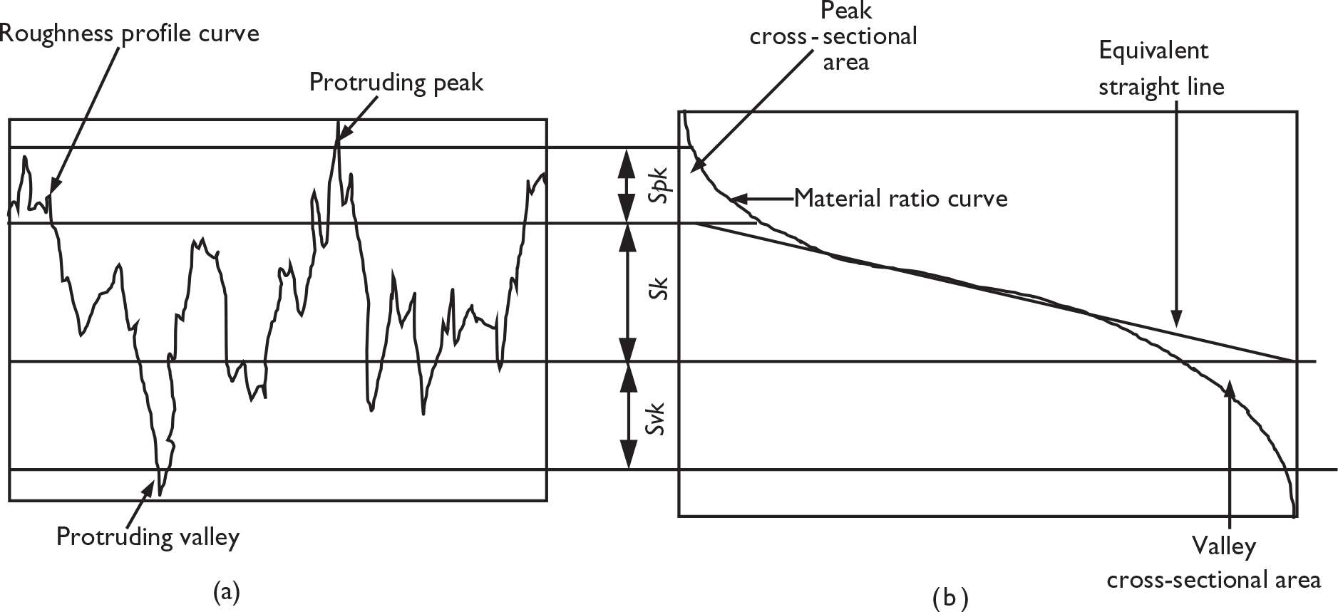
Sk. Sk, that is, core roughness depth as shown in Figure 1 measures the height between peak and valley of the surface after removal of the predominant peaks and valleys.⁴ Lower core roughness depth indicates better wear properties. Hence, a small value of the final Sk implies better wear properties of the knee implant.

Svk. Svk, that is, reduced valley depth measures the valley depth below core roughness as shown in Figure 1.⁴ The presence of valley increases body fluid retention capability, which results in better femoral implant performance. Hence, a higher value of Svk means better performance of the implant material.

To achieve required surface roughness and surface topography for femoral knee implant, various polishing processes are employed. Commercially, grinding, drag finishing, vibratory finishing systems and other processes are used to finish femoral component of a knee implant. To provide better surface roughness and surface topography, various researchers proposed different methods. Mechanochemical method is proposed to obtain necessary surface finish of knee implant.⁵ Zeeko polishing machine is used to polish femoral knee implant with nanoscale surface roughness and surface topography.⁶ Also, abrasive flow finishing process is used to finish femoral knee implant.⁷ These processes provide nanometer-level surface finishing on femoral knee implant. However, precise control of the finishing forces is not possible in the above-mentioned processes. Magnetorheological (MR) fluid-based finishing processes provide precision finishing due to the proper control of the finishing forces. Magnetic field assisted finishing (MFAF) process uses MR fluid mixed with diamond abrasive powder as a finishing medium. MR fluid is a blend of carbonyl iron particles (CIPs) and abrasive particles in a continuous phase base medium.⁸ MR fluid changes its rheological properties under the application of external magnetic field by forming chain structure along the magnetic field lines.⁹ Many researchers contributed to the advancement of MR fluid-based finishing process. Generally, optics are finished using this process.^10–¹² This process generates Ǻ level surface roughness in different type of optics surface without sub-surface damage.¹³ Although this process was primarily used for finishing optics, some researchers used this process to finish different types of metals.^14–¹⁶ This process also gives nanometer-level surface finish in metal workpieces.¹⁷ Some researchers also used MR fluid-based finishing processes to finish femoral knee joint.^18, ¹⁹ To further increase the process efficiency, a new MFAF experimental setup is developed. In the present study, the developed tool is used to obtain uniform finishing on freeform surfaces.

Response surface methodology (RSM) of statistical design of experiments (DOE) is carried out²⁰ in the current study. The plan of the experiments is based on central composite rotatable design (CCRD) of RSM. This method is very efficient to achieve optimal process performance.²⁰ In RSM, a minimum number of experiments will provide the maximum amount of information about the process.

In the present study, the objective is to optimize the process parameters in order to obtain the minimum value of Sa, Spk, Sk and the maximum value of Svk. CCRD is used to optimize the input process parameters to acquire necessary 3D surface roughness parameter values for Ti alloy. Optimization of the process parameters of MFAF process will give necessary surface finish and surface topography for higher performance and longevity of femoral knee joint implant after finishing with MFAF process. Also, the effect of each process parameter on output responses is analyzed for better understanding of the finishing process. After that, validation experiments are conducted to confirm the optimization results obtained from the DOE study. Optical profilometer, field emission scanning electron microscope (FESEM) and atomic force microscope (AFM) images are used to analyze the surface roughness and surface topography of the components.

MFAF experimentation

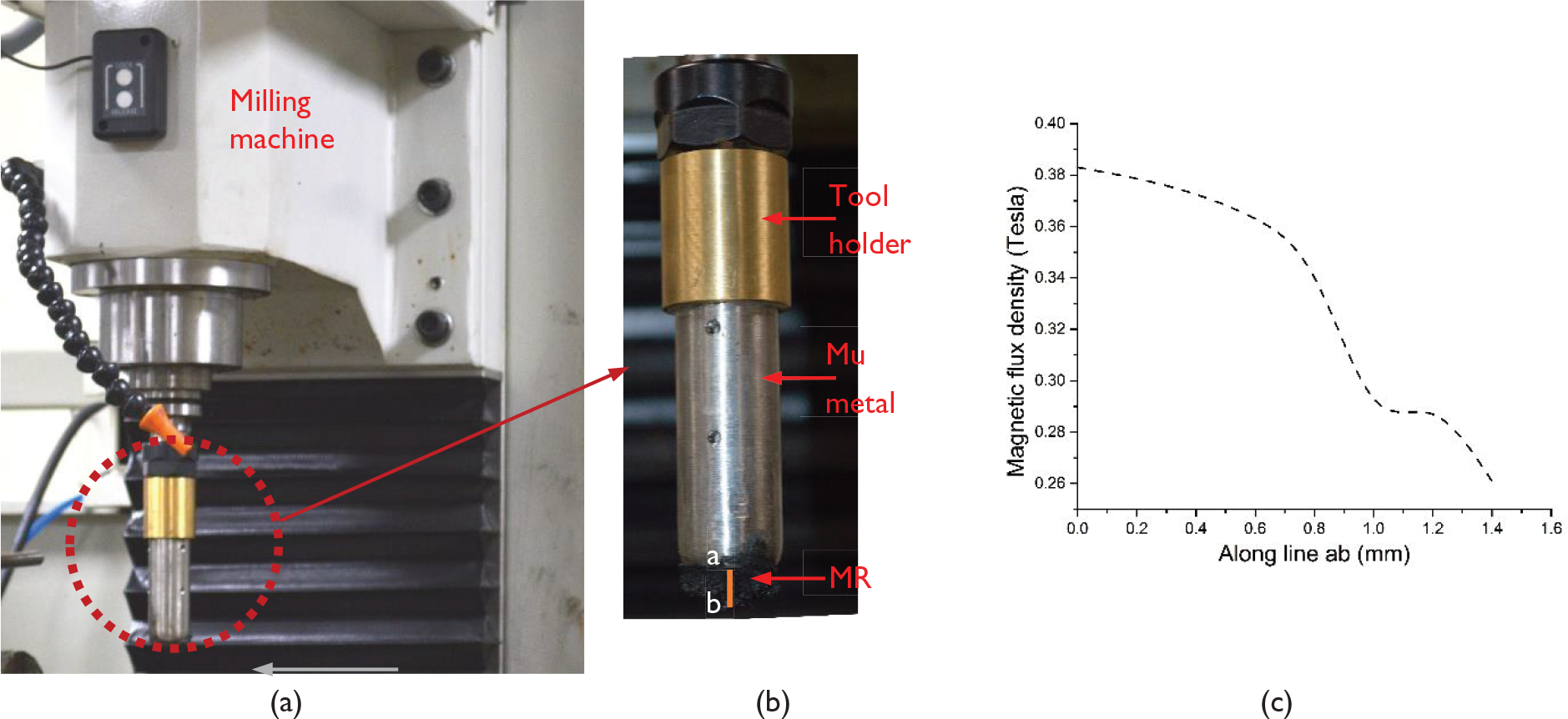
MFAF experimental setup and the novel developed tool is shown in Figure 2.²¹ The polishing tool is shown in Figure 2(b) is specially designed to carry out the finishing operation in MFAF process. The tool consists of Nd-Fe-B (N48 grade) permanent magnet inserted inside a magnet holder made of mu-metal. A four-axis vertical CNC milling machine holds the tool during finishing (Figure 2(a)). Ti alloy (Ti-6Al-4V) of grade 5 is used as the workpiece. Figure 2(c) shows the measured magnetic flux density along line ab (Figure 2(b)). As shown in Figure 2(c), near the tool tip, the available magnetic flux density is 0.38 Tesla. However, the available magnetic flux density reduces to 0.2 Tesla at 1.4-mm distance away from the tool tip. The workpiece is held with a precision vice during the finishing operation.

Figure 2.

(a) Magnetic field assisted finishing experimental setup, (b) novel developed tool and (c) measured magnetic flux density from tool-tip along line ab (Figure 2(b)).

The MR polishing fluid comprises of CIP (40 vol%) of EN grade (8 µm) from BASF, Germany and diamond abrasive particles (7.1 vol%) of size 6 µm in the base medium. The base medium consists of 3 ml hydrofluoric acid, 6 ml nitric acid (HNO₃) and 100 ml distilled water.²² The base medium is selected based on workpiece physical properties. The acidic base medium is chosen due to the high hardness of the Ti alloy. The base medium makes the workpiece surface soft which helps abrasive particles to easily indent and remove material from the workpiece surface. The schematic diagram of the developed tool along with MR fluid and Ti alloy workpiece is shown in Figure 3(a). The contour plot of magnetic field distribution during finishing is shown in Figure 3(b).

Figure 3.

(a) Schematic diagram of novel developed tool along with MR fluid and bio-titanium workpiece and (b) contour plot of magnetic field distribution during finishing.

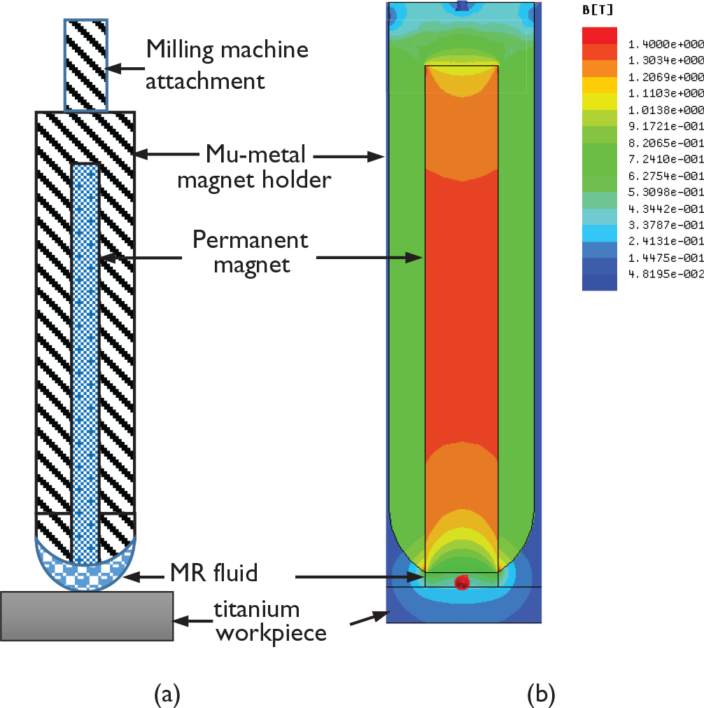
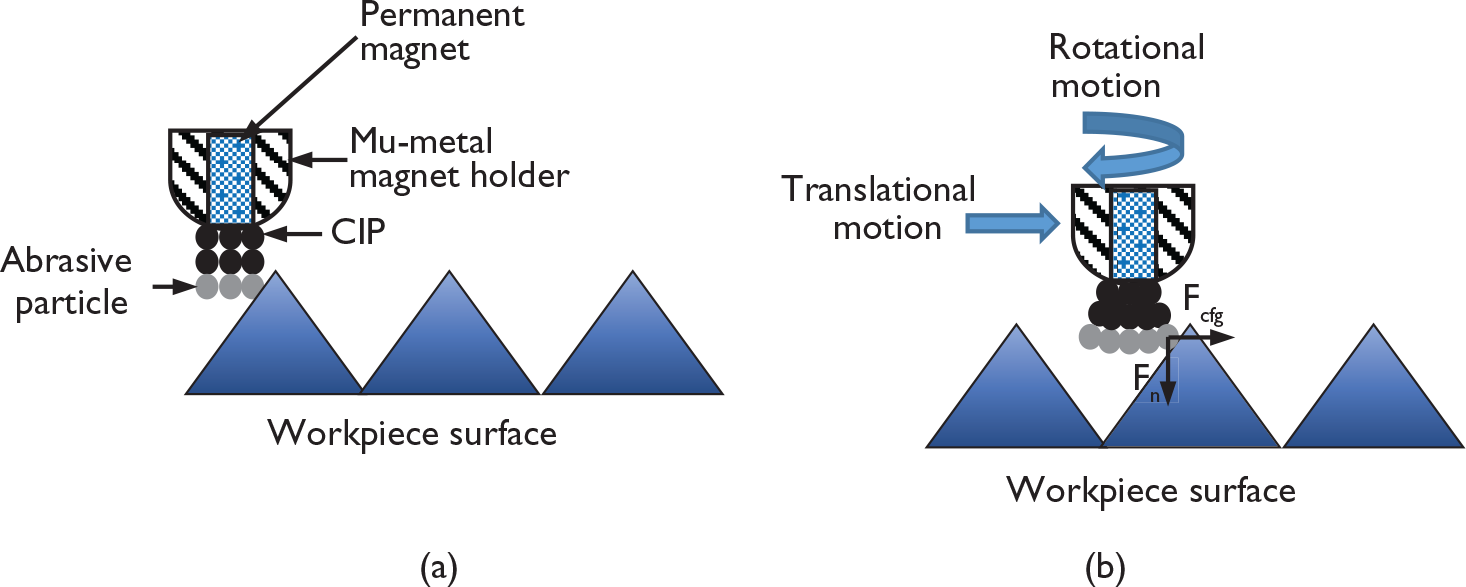
Figure 4 explains the mechanism of polishing using MR fluid in MFAF process. Figure 4(a) shows the CIPs and abrasive particles below the polishing tool just before starting the finishing operation where the CIP chains are not sheared at all. The chain structure formed by CIPs follows the magnetic lines of force. The CIPs are attracted to the magnet pole due to its magnetic property. On the other hand, the abrasive particles are situated at the far end of the CIPs chain structure away from magnet pole. Magnetic levitation force is responsible for this behavior of the MR fluid.²³ Figure 4(b) shows the MR fluid chain structure and also the forces applied on the abrasive particles, which are responsible for cutting the roughness peaks from the workpiece surface. In Figure 4(b), due to the rotational motion of the tool, the MR fluid chains move in the outward direction. With higher rpm, the MR fluid chains break due to the decrease in finishing medium viscosity with increasing shear rate. Figures 5(a) and (b) show the MR fluid chain formation just below the tool and at the edge of the novel developed tool, respectively. Under pressure and also due to the rotational motion of the tool, the MR fluid forms the particular structure as shown in Figure 5(a). At the edge of the tool, the chain structure forms an arc shape as shown in Figure 5(b).

Figure 4.

MFAF tool along with MR fluid (a) before finishing and (b) during finishing with different forces (F_n: normal force and F_cfg: centrifugal force) responsible for finishing operation.

Figure 5.

MR fluid chain formation (a) below and (b) at the edge of the novel developed tool.

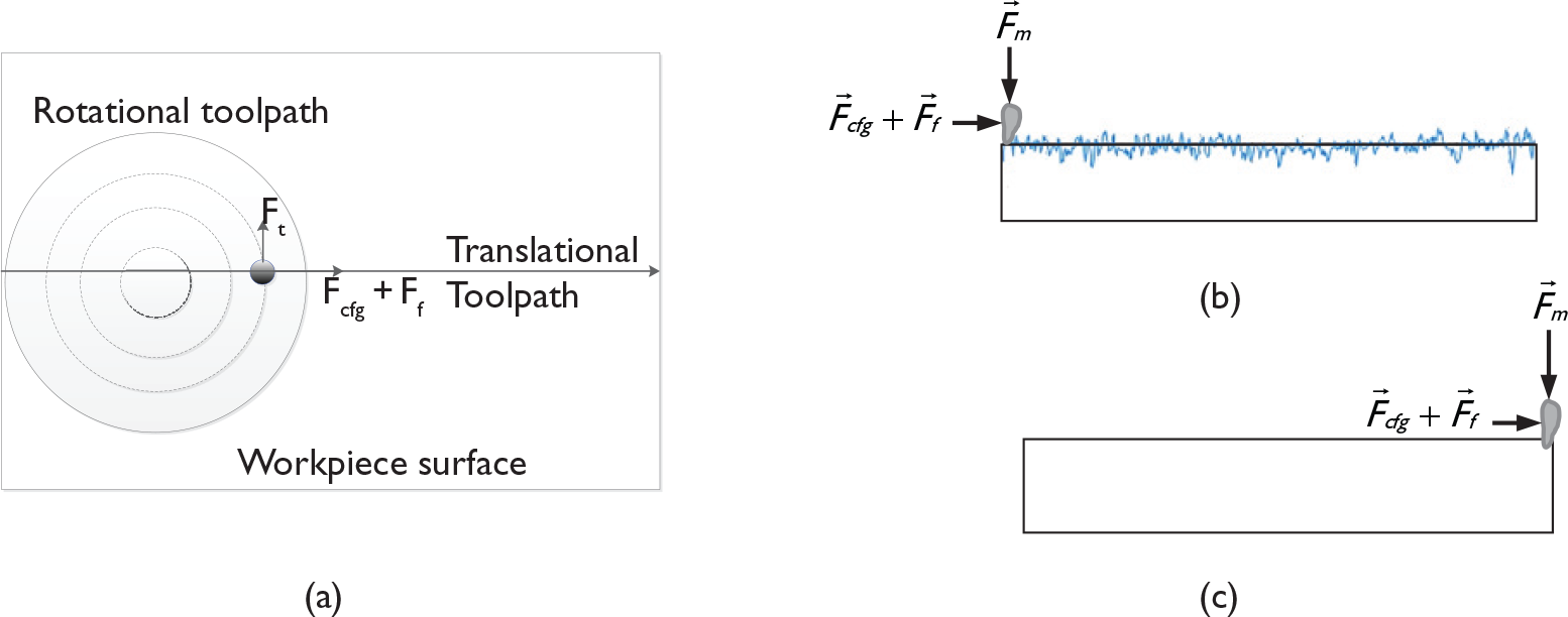
A CNC toolpath is generated and further optimized to guide the tool during finishing. Both translational and rotational motions are provided to the tool as shown in Figure 6(a) to uniformly finish the workpiece. The circular path of the abrasive in Figure 6(a) is formed due to the formation of the particular shape of the MR fluid below the tool as shown in Figure 5(a). Centrifugal (F_cfg) force acts on the abrasive particles as a result of the rotating tool as shown in Figure 6(a). Feed force (F_f) helps the abrasive particles to shear the indented material from the workpiece surface that is generated due to the translational motion of the tool along the tool path (Figure 6(a)). Figure 6(b) shows an active abrasive particle started cutting the roughness peak along the surface roughness profile while indenting into it. The generated surface profile (Figure 6(c)) is due to the shearing of peaks by abrasive particles. As shown in Figures 6(b) and (c), two main forces are acting on the abrasive particles during the finishing process. The abrasive particles indent on the workpiece surface because of the applied normal force, that is, the magnetic force (F_m) through the surrounding CIP chains. The abrasive particles shear the indented material with the help of centrifugal (F_cfg) and feed (F_f) forces. These forces help in removing surface undulations from the workpiece surface.

Figure 6.

(a) Toolpath and forces acting on active abrasive particle due to rotational and translational motions of the tool during finishing; surface profile of the component and normal and shear forces acting on abrasive particle (b) before and (c) after MFAF process.

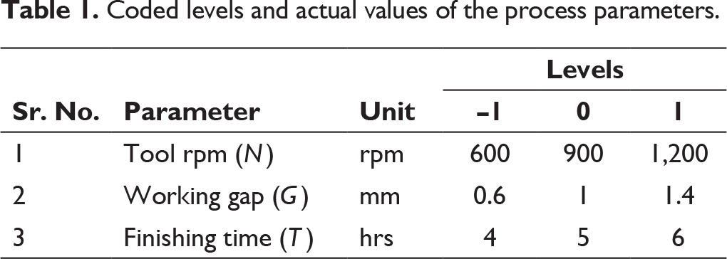
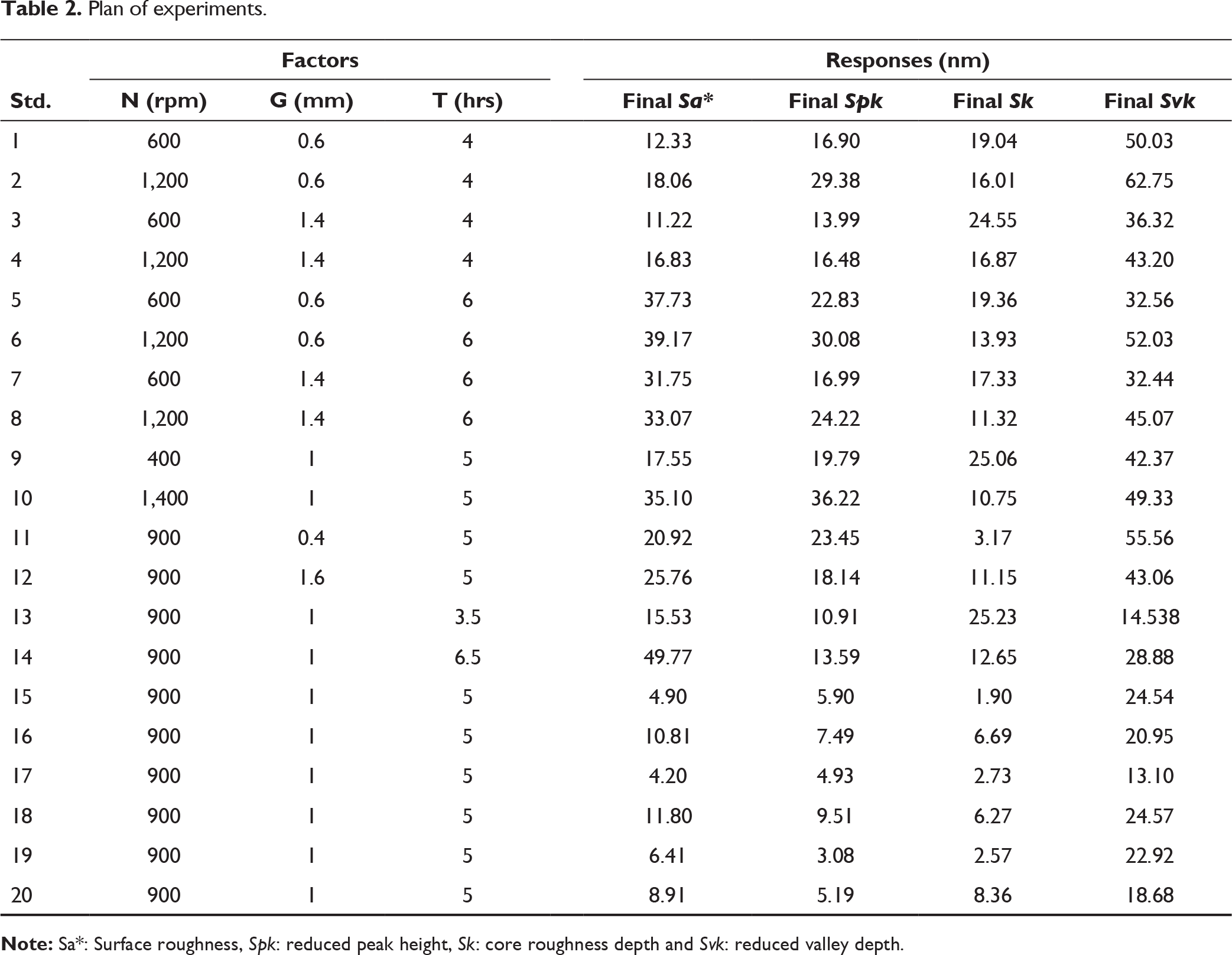
From the preliminary experimental study, it is observed that the main influential process parameters in MFAF process are rpm of the tool (N), working gap between tool and workpiece (G) and finishing time (T ). The 3D surface roughness parameters (i.e. height and functional parameters) are considered as output responses. The range of each process parameters with coded levels and actual values are given in Table 1. The plan of experiments along with all the responses is shown in Table 2. All the surface roughness parameters are measured before and after the experiments using optical profilometer. The initial Sa values of all the workpiece are in the range of 70–80 nm having minor variation. Hence, the final value of the 3D surface parameters after finishing is considered as responses because the difference between initial surface roughness of the workpiece is uniform. The final surface roughness parameter values are sufficient to interpret the surface roughness and topography of the workpiece.

Table 1.

Coded levels and actual values of the process parameters.

Sr. No.	Parameter	Unit	Levels
Sr. No.	Parameter	Unit	–1	0	1
1	Tool rpm (N )	rpm	600	900	1,200
2	Working gap (G )	mm	0.6	1	1.4
3	Finishing time (T )	hrs	4	5	6

Table 2.

Plan of experiments.

	Factors			Responses (nm)
Std.	N (rpm)	G (mm)	T (hrs)	Final Sa *	Final Spk	Final Sk	Final Svk
1	600	0.6	4	12.33	16.90	19.04	50.03
2	1,200	0.6	4	18.06	29.38	16.01	62.75
3	600	1.4	4	11.22	13.99	24.55	36.32
4	1,200	1.4	4	16.83	16.48	16.87	43.20
5	600	0.6	6	37.73	22.83	19.36	32.56
6	1,200	0.6	6	39.17	30.08	13.93	52.03
7	600	1.4	6	31.75	16.99	17.33	32.44
8	1,200	1.4	6	33.07	24.22	11.32	45.07
9	400	1	5	17.55	19.79	25.06	42.37
10	1,400	1	5	35.10	36.22	10.75	49.33
11	900	0.4	5	20.92	23.45	3.17	55.56
12	900	1.6	5	25.76	18.14	11.15	43.06
13	900	1	3.5	15.53	10.91	25.23	14.538
14	900	1	6.5	49.77	13.59	12.65	28.88
15	900	1	5	4.90	5.90	1.90	24.54
16	900	1	5	10.81	7.49	6.69	20.95
17	900	1	5	4.20	4.93	2.73	13.10
18	900	1	5	11.80	9.51	6.27	24.57
19	900	1	5	6.41	3.08	2.57	22.92
20	900	1	5	8.91	5.19	8.36	18.68

Note: Sa*: Surface roughness, Spk: reduced peak height, Sk: core roughness depth and Svk: reduced valley depth.

Results and discussion

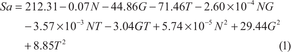
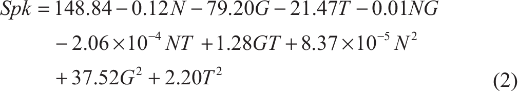
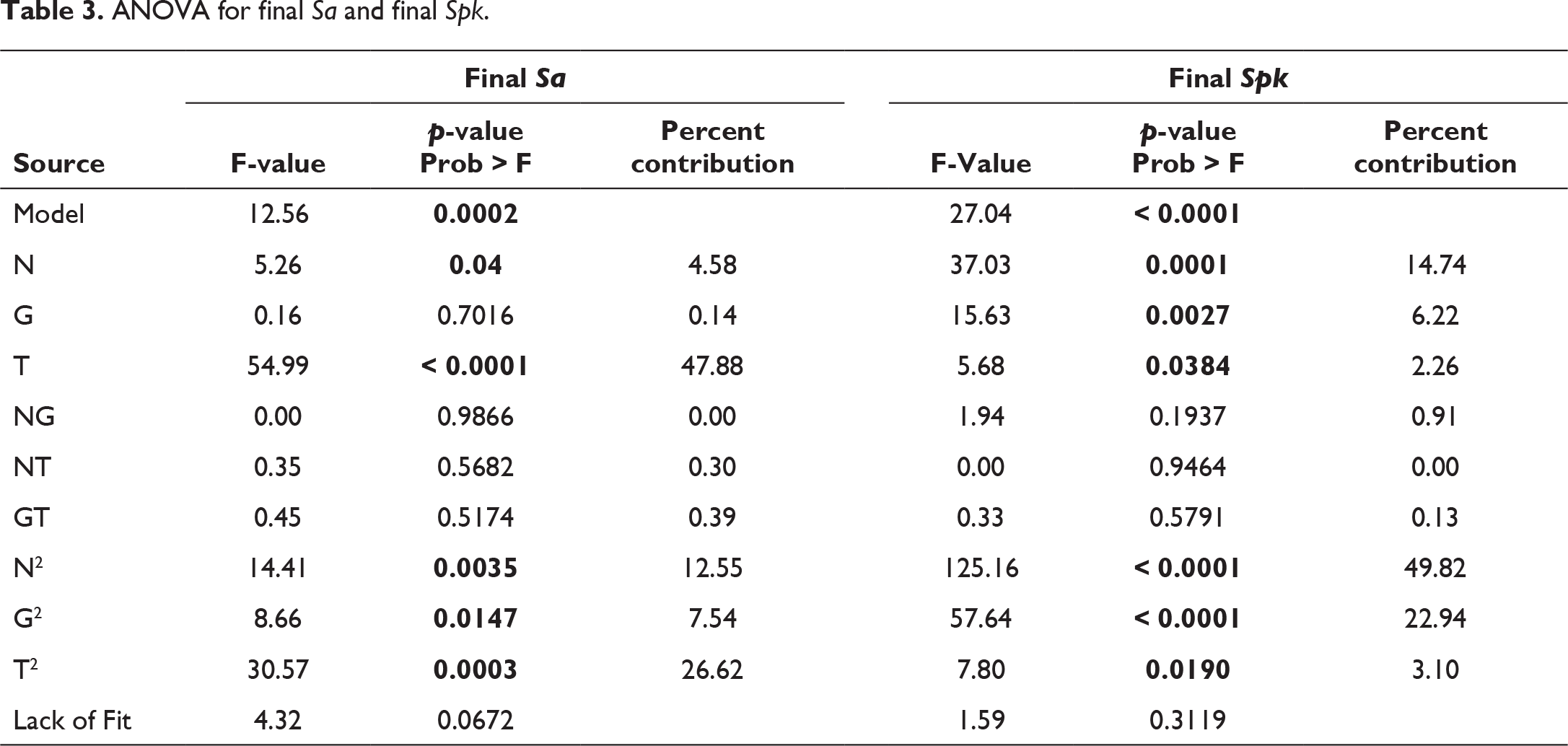
Analysis of variance (ANOVA) for final Sa and final Spk is shown in Table 3. ANOVA table helps to understand the significance of the developed model and the impact of the process parameters on the responses. In Table 3, ANOVA models for both final Sa and final Spk are significant as p values (‘Prob > F’) for both the cases are less than 0.05 for 95% significance level. For final Sa, the significant model terms are N, T, N², G² and T². The significant model terms for final Spk are N, G, T, N² ,G² and T². Also, it is found that ‘Lack of Fit’ relative to the pure error is insignificant for both the cases. In case of Sa, the most significant term is T, that is, finishing time with highest contribution (47.88%) followed by T², that is, square of the finishing time (26.62% contribution) and N², that is, square of rpm of the tool (12.55% contribution). For final Spk, the contribution of the most significant terms in descending order is square of the rpm of the tool (49.82% contribution), square of the working gap (22.94% contribution) and finishing time (14.74% contribution). The co-efficient of determination (R²) value in case of final Sa is 0.92 and in case of final Spk is 0.96, which shows good fitting of the regression equation with the experimental results. From regression analysis, the response surface models for final Sa and final Spk are given in Equations (1) and (2), respectively.

\begin{array}{l} S a = 212.31 - 0.07 N - 44.86 G - 71.46 T - 2.60 \times 10^{- 4} N G \\ - 3.57 \times 10^{- 3} N T - 3.04 G T + 5.74 \times 10^{- 5} N^{2} + 29.44 G^{2} + 8.85 T^{2} \end{array}

(1)

\begin{array}{l} S p k = 148.84 - 0.12 N - 79.20 G - 21.47 T - 0.01 N G \\ - 2.06 \times 10^{- 4} N T + 1.28 G T + 8.37 \times 10^{- 5} N^{2} + 37.52 G^{2} + 2.20 T^{2} \end{array}

(2)

Table 3.

ANOVA for final Sa and final Spk.

	Final Sa			Final Spk
Source	F-value	p-value Prob > F	Percent contribution	F-Value	p-value Prob > F	Percent contribution
Model	12.56	0.0002		27.04	< 0.0001
N	5.26	0.04	4.58	37.03	0.0001	14.74
G	0.16	0.7016	0.14	15.63	0.0027	6.22
T	54.99	< 0.0001	47.88	5.68	0.0384	2.26
NG	0.00	0.9866	0.00	1.94	0.1937	0.91
NT	0.35	0.5682	0.30	0.00	0.9464	0.00
GT	0.45	0.5174	0.39	0.33	0.5791	0.13
N²	14.41	0.0035	12.55	125.16	< 0.0001	49.82
G²	8.66	0.0147	7.54	57.64	< 0.0001	22.94
T²	30.57	0.0003	26.62	7.80	0.0190	3.10
Lack of Fit	4.32	0.0672		1.59	0.3119

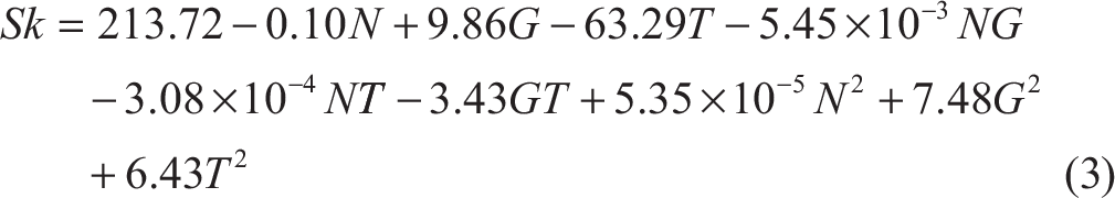
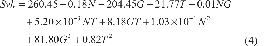
As shown in Table 4, ANOVA models for both Sk and Svk are significant. For Sk,, the most significant model terms in descending order are T² (40.59%), N² (31.43%) and N (14.88%) while for Svk the most significant model terms are G² (47.59%), N² (33.16%) and N (7.97%). Also, ‘lack of fit’ for both Sk and Svk are insignificant relative to the pure error. The R² value for Sk and Svk are 0.93 and 0.90, respectively, which proves that the regression line approximates the real data points very well. From regression analysis, the response surface models for Sk and Svk are given in Equations (3) and (4), respectively.

\begin{array}{l} S k = 213.72 - 0.10 N + 9.86 G - 63.29 T - 5.45 \times 10^{- 3} N G \\ - 3.08 \times 10^{- 4} N T - 3.43 G T + 5.35 \times 10^{- 5} N^{2} + 7.48 G^{2} \\ + 6.43 T^{2} \end{array}

(3)

\begin{array}{l} S v k = 260.45 - 0.18 N - 204.45 G - 21.77 T - 0.01 N G \\ + 5.20 \times 10^{- 3} N T + 8.18 G T + 1.03 \times 10^{- 4} N^{2} \\ + 81.80 G^{2} + 0.82 T^{2} \end{array}

(4)

Table 4.

ANOVA for final Sk and final Svk.

Source	Final Sk			Final Svk
Source	F-value	p-value Prob > F	Percent contribution	F-value	p-value Prob > F	Percent contribution
Model	14.20	0.0001		10.58	0.0005
N	19.57	0.0013	14.88	7.82	0.0189	7.97
G	1.89	0.1993	1.44	7.40	0.0216	7.54
T	11.17	0.0075	8.49	0.16	0.6979	0.16
NG	0.43	0.5267	0.38	0.53	0.4822	0.59
NT	0.01	0.9280	0.01	0.52	0.4884	0.53
GT	1.90	0.1986	1.44	2.27	0.1628	2.31
N²	41.36	< 0.0001	31.43	32.55	0.0002	33.16
G²	1.85	0.2034	1.41	46.71	< 0.0001	47.59
T²	53.41	< 0.0001	40.59	0.18	0.6772	0.19
Lack of Fit	1.21	0.4210		2.91	0.1330

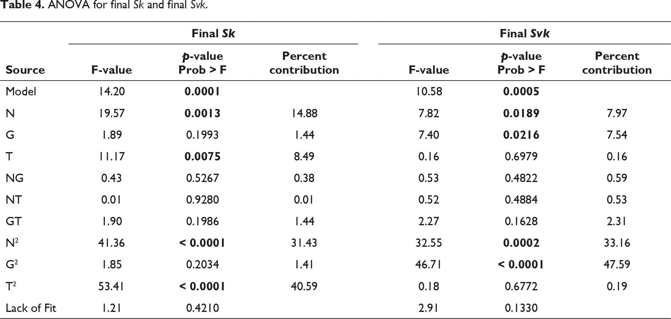
Hence, from ANOVA for all the responses (Tables 3 and 4), it can be concluded that the square of the working gap between the tool and workpiece is the most significant process parameter to control surface finish, wear capability and performance criteria of the implant.

An optimization study is carried out based on Derringer and Suich’s algorithm²⁴ considering multiple responses is used to conduct an optimization study. This algorithm uses desirability functions. The results of the optimization study are given in Table 5. From Table 5, it can be concluded that to achieve optimum 3D surface parameter values, the rotation speed of the tool should be 901.63 rpm with a working gap of 0.6 mm and finishing time of 4.65 hrs. The effect of each process parameter on surface roughness and surface topography is discussed in the next sub-section.

Effect of process parameters on output responses

The effects of individual process parameter on output responses are calculated using regression equations (Equations (1–4)). The effect of tool rpm on Sa, Spk,Sk, and Svk are shown in Figures 10–13. With the increase in rpm of the tool, the values of the 3D surface roughness parameters start to decrease till it reaches a certain speed. Beyond that particular speed, the 3D surface roughness parameter values start to increase with increasing tool rpm. Centrifugal force (F_cfg) acts as a finishing force in MFAF process. It depends on the tool rpm. The centrifugal force (F_cfg) acting on an abrasive particle is given as²⁵

F c f g = m {(\frac{2 π N}{60})}^{2} r

(5)

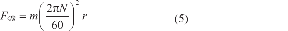
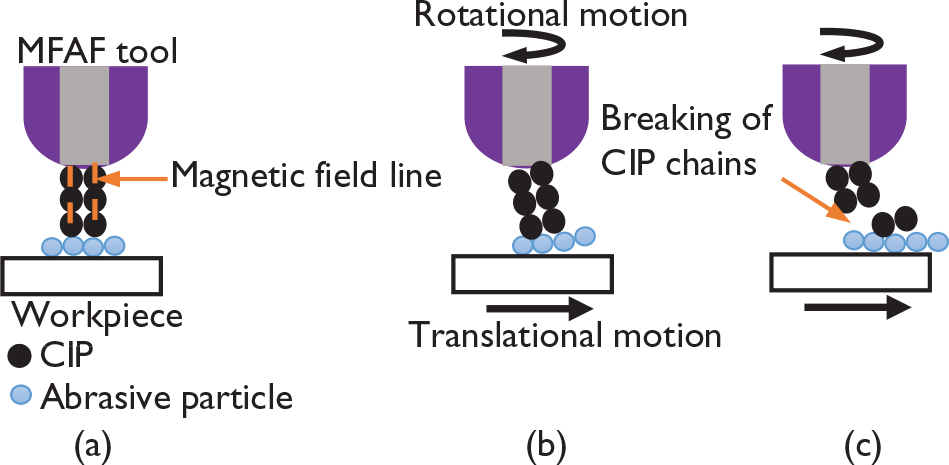
where m is the mass of the abrasive particle, N is the rpm of the tool and r is the distance between the axis of the cylindrical tool and a particular abrasive particle. Hence, the finishing force (i.e. F_cfg) acting on the abrasive particle increases with the increase in the tool rpm. The increased finishing force results in a higher material removal from the roughness peaks. Hence, with the increase in tool rpm, final Sa, Spk,Sk, and Svk values decrease. The value of F_cfg increases further with higher tool rpm. Due to the growing force, the CIP chains start to break due to the shear thinning nature of MR fluid, and then the abrasive particles break loose from the CIP chain structures and move into the outward direction from the finishing zone. It is explained clearly with the help of schematic diagrams in Figure 7. In Figure 7(a), unyielded CIP chains are observed while there is no shear force like tool rotation or translational motion of the workpiece. The CIP chains are started to shear without breakage with slight increase in tool rpm as shown in Figure 7(b). However, at high rpm ( > 1100 rpm), shearing force also becomes very high which leads to breakage in chain structure and it gets little time to recombine as shown in Figure 7(c). Hence, the strength of the CIP chains reduces due to the breaking of the chains and the CIP chains do not provide sufficient bonding force to the abrasive particles for cutting the roughness peaks. It results in a lower material removal. Hence, higher value of final 3D surface roughness parameters is observed.

Figure 7.

CIP chains and abrasive particles in MR fluid below MFAF tool under (a) static condition, (b) nominal shearing condition and sheared chains without breaking and (c) high shearing condition and breaking of chains.

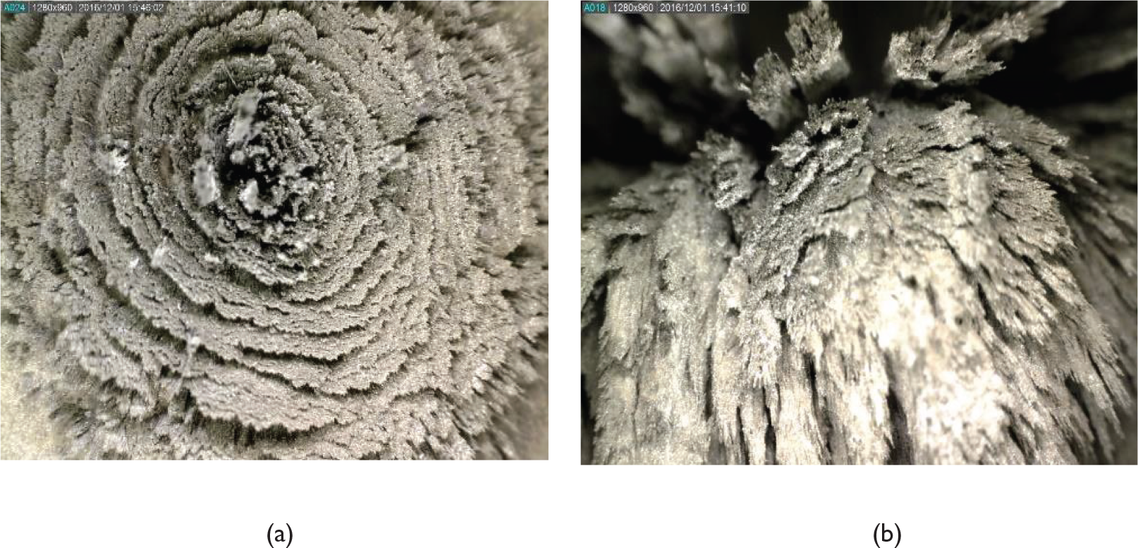
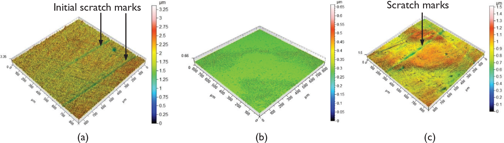
As shown in the Figures 10–13, the effect of working gap on final Sa, Spk,Sk, and Svk is significant. Initially, final 3D surface roughness parameter values start to decrease with the increase in the working gap and it reaches to a particular value. Increasing working gap means there is an increase in the available abrasive particles in the finishing zone resulting in higher material removal. Higher material removal gives low final Sa, Spk,Sk, and Svk values. However, further increase in the working gap beyond this particular working gap, the final Sa, Spk,Sk, and Svk values start to increase. With an increase in the working gap, there is a reduction in magnetic force on the abrasive particles through surrounding CIP chains, which results in the lower indentation of the abrasive particles on the workpiece surface. Hence, penetration depth by the abrasive particle decreases resulting in an increase in final Sa, Spk,Sk, and Svk values. The effect of working gap on 3D surface topography of the workpiece is shown in Figure 8. The initial unfinished workpiece surface shows deep scratch marks as shown in Figure 8(a). Finishing experiments are carried out at 1 mm (Figure 8(b)) and 1.4 mm (Figure 8(c)) working gaps with tool rpm of 1000 and 4 hrs of finishing time. The surface topography in Figure 8(b) for 1-mm working gap shows no scratch marks with low roughness peaks and thus a very good surface finish is achieved. However, the generated surface topography (Figure 8(c)) for 1.4-mm working gap shows the presence of initial scratch marks which MR polishing fluid could not remove properly. It proves that at 1.4-mm working gap, the finishing capability of abrasive particles reduces. It happens due to the insufficient magnetic flux density in the finishing zone. The available magnetic flux density under the tool after 1.4-mm working gap is less than 0.2 T which is not enough to carry out the finishing operation efficiently.²¹

Figure 8.

3D surface topography of workpieces: (a) before finishing, for (b) 1 mm and (c) 1.4-mm working gap with 1000 tool rpm and 4 hrs finishing time

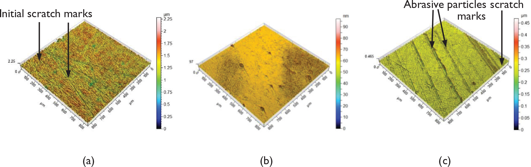
Figures 10–13 show the effect of finishing time on output responses. Initially, final Sa, Spk,Sk, and Svk values start to decrease with an increase in the finishing time until it reaches an optimum value. However, beyond the optimum value, 3D surface roughness parameter values start to increase with a further increase in the finishing time. At first, with the increase in the finishing time, the abrasive particles get more time to finish the surface resulting in low 3D surface roughness parameter values. After the optimum finishing time, the abrasive particles rub the already finished surface resulting in an increase in the response parameters. The effect of finishing time on 3D surface topography of the workpiece is shown in Figure 9. The initial surface topography with high peaks and deep valleys is shown in Figure 9(a). Here, the experiments are carried out at 1000 tool rpm and 1-mm working gap. After finishing for 4.5 hrs, the generated surface has little scratch marks than the initial surface with reduced surface roughness as shown in Figure 9(b). After finishing for 6 hrs, abrasive particles start to scratch the already finished surface which deteriorates the finishing performance as shown in Figure 9(c).

Figure 9.

3D surface topography of workpieces: (a) before finishing, after (b) 4.5 hrs and (c) 6 hrs finishing time with 1000 tool rpm and 1-mm working gap.

Effect of process parameters on final Sa

Sa determines the overall surface roughness of the implant material. Hence, lower value of final Sa implies overall good surface finish of the component. Effect of tool rpm on final Sa is shown in Figures 10(a) and (c) where it is observed that with the increase in tool rpm, the final Sa starts to decrease. However, beyond 900 rpm, the final Sa starts to increase. The reason for which is already explained in Section 3.1. The final surface roughness differs at different working gaps for a certain tool rpm as shown in Figure 10 (c). At 0.6-mm working gap, the value of surface roughness is higher because of less amount of abrasive particle in the finishing zone. At 1-mm working gap, increase in the available active abrasive particles result in a decrease in final surface roughness. At 1.4-mm working gap, the magnetic force responsible for indenting the abrasive particle reduces. Hence, the material removal starts to decrease which increases the final Sa value.

Figure 10.

3D graph showing the combined effect of (a) rpm of the tool and working gap and (b) working gap and finishing time on final surface roughness (Sa); the effect of (c) rpm of the tool at different working gap and (d) working gap at different finishing time on final Sa.

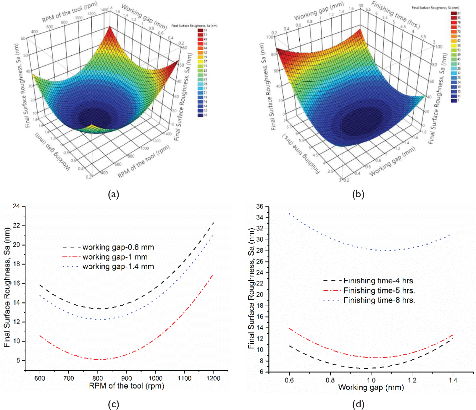
Effect of working gap on final Sa is shown in Figures 10(a), (b), (c) and (b). With the increase in working gap, final Sa values start to decrease due to the increase of active abrasive particles in the finishing zone. The increased amount of active abrasive particles removes more material resulting in low final Sa values. However, after a 1.2-mm working gap, final Sa values start to increase due to the reduction of magnetic force acting on the abrasive particles. As shown in Figure 10(d), for the same working gap, the final Sa values are different at different finishing time. Hence, the finishing capability of the abrasive particles decreases resulting in lower material removal rate, which in turn increases final Sa values.

Effect of finishing time on final Sa values are shown in Figures 10(b) and (d). After 5.5 hrs of finishing time, the final Sa values start to increase at a higher rate due to the longer finishing time. With a longer finishing time, the abrasive particles start to abrade the already finished workpiece surface, which increases final Sa values. Hence, to achieve good surface finish for Ti alloy implant, the range of tool rpm, working gap and finishing time should be in the range of 800–1000 rpm, 0.8–1.2 mm and 4–5 hrs, respectively.

Effect of process parameters on final Spk

Wear properties of bearing surfaces of femoral knee implant greatly depends on final Spk values. Low final Spk value implies good wear properties, which are required for the use of Ti alloy as a femoral knee joint implant. Effect of tool rpm on final Spk is shown in Figures 11(a) and (c) where it is observed that with the increase in the tool rpm, the final Spk starts to decrease. However, beyond 900 rpm with the increase in tool rpm, the final Spk starts to increase. As Spk represents the mean height of peaks above the core surface, the increasing tool rpm helps in shearing of the roughness peaks, which decreases the final Spk values. After 900 rpm, the shearing of the peaks starts to decrease due to the weak bonding of the active abrasive particles in the finishing zone, which increases the final Spk values. As shown in Figure 11(c), the final Spk is different at different working gaps for the same tool rpm. At 0.6-mm working gap, the amount of active abrasive particle in the finishing zone is low resulting in lower rate of peak shearing. At 1-mm working gap, the available active abrasive particle increases that results in higher rate of peak shearing which decreases the final Spk values. At 1.4-mm working gap, the magnetic force responsible for indenting of abrasive particle reduces which lowers the peak shearing capability of abrasive particles resulting in higher final Spk values than 1-mm working gap.

Figure 11.

3D graph showing the combined effect of (a) finishing time and rpm of the tool and (b) finishing time and working gap on final reduced peak height (Spk); the effect of (c) rpm of the tool and (d) finishing time on final Spk at different working gap.

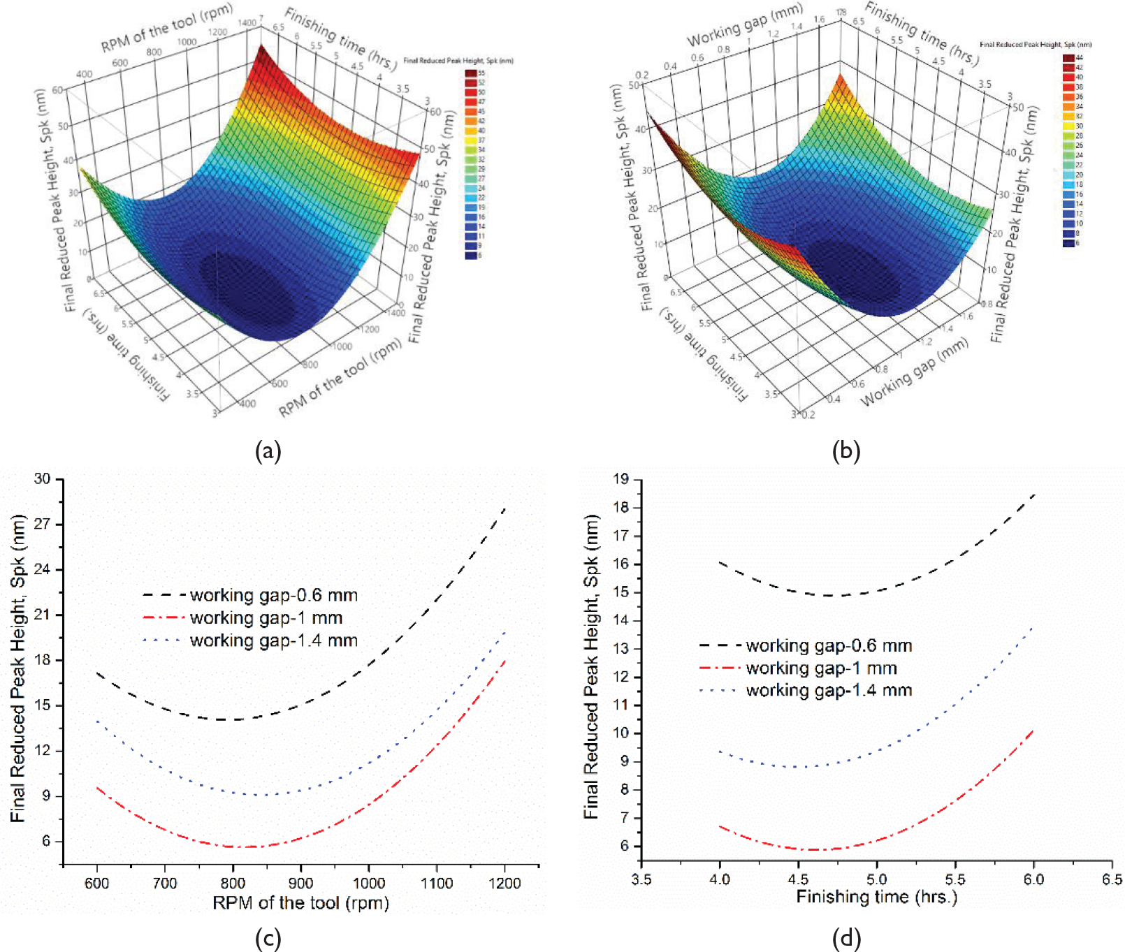
Effect of working gap on Spk is shown in Figures 11(b), (c) and (d). With the increase in working gap, final Spk values start to decrease, however, after 1.2-mm working gap, it starts to increase. The reason behind these is already explained in the previous paragraph.

Figures 11(a), (b) and (d) show the effect of finishing time on final Spkvalues. From 4 to 5 hrs finishing time, the final Spk values start to decrease with increasing finishing time. This increases the interaction time of active abrasive particles with the workpiece surface, which results in more shearing of peaks. After 5 hrs of finishing time, final Spk value starts to increase because the abrasive particles start to plow the finished surface resulting in higher peaks. Hence, to achieve good wear properties rpm of the tool, working gap and finishing time should be in the range of 700–900 rpm, 0.9–1.2 mm and 4–5 hrs, respectively, during MFAF process.

Effect of process parameters on final Sk,

Low Sk value implies less wear of the femoral knee joint implant during in-vivo performance. From the Figures 12(a) and (c), it is observed that with the increase in tool rpm, the final Sk values start to decrease, however, beyond 1100 rpm, its value starts to increase. Final Sk value is calculated by subtracting the minimum height from the maximum height of the core surface. Now, with the increase in tool rpm, the material removal capability of abrasive particles increase. These result in decreasing the difference between maximum and minimum height of the core surface. Due to this, the final Spk values start to decrease. However, after 1100 rpm due to the reduction of finishing capability of abrasive particles, the difference between maximum and minimum height of the core surface starts to increase resulting in higher final Sk values.

Figure 12.

3D graph showing the combined effect of (a) rpm of the tool an d finishing time and (b) finishing time and working gap on final core roughness depth (Sk); the effect of (c) rpm of the tool at different finishing time on final Sk.

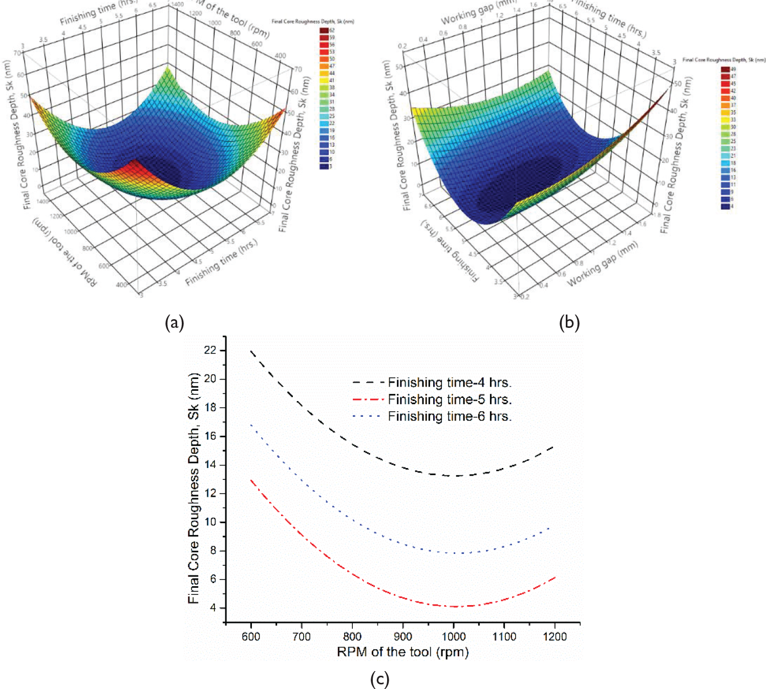
Effect of working gap on final Sk values is shown in Figure 12(b). Final Sk values start to decrease up to 1.2-mm working gap. Increasing working gap implies higher amount of active abrasive particles in the finishing zone, which helps to reduce difference between minimum height and maximum height. However, after 1.2-mm working gap, the final Sk values start to increase with the increase in working gap due to the reduction in finishing force.

The effect of finishing time on final Sk values is shown in Figures 12(a), (b) and (c). Initially, with the increase in finishing time, the final Sk values start to decrease, however, after 5.5 hrs, the final Sk values start to increase with increasing finishing time. Before 5.5 hrs finishing time, the abrasive particles finish the workpiece surface by reducing the peak height which in turn diminishes the maximum and minimum height difference resulting in lower final Sk values. After 5.5 hrs, the abrasive particles start to abrade the already finished workpiece resulting in unwanted scratch marks. These escalate the difference between the maximum and minimum height implying increase in the final Sk values. As shown in Figure 12(d), for same tool rpm, final Sk values are different for different finishing time. Hence, to achieve better performance and wear properties for Ti alloy implant rpm of the tool, the working gap and finishing time should be in the range of 800–1100 rpm, 0.8–1.2 mm and 4.5–5.5 hrs, respectively.

Effect of process parameters on final Svk

For better performance of the Ti alloy implant, final Svk values should be high. Effect of tool rpm on final Svk is shown in Figures 13(a) and (c). With the increase in tool rpm, the final Svk values start to decrease, however, beyond 900 rpm, the final Svk values increase. Svk represents the mean depth of the valleys below the core surface. The finishing capability of the abrasive particles grows due to the increase in tool rpm, which increases the material removal rate. Due to these, the valley depth decreases resulting in lower final Svk values. After 900 rpm, the abrasive particles start to rub the workpiece surface, which results in increased valley depth making higher values of final Svk.

Effect of working gap on final Svk value is shown in Figures 13(a), (b) and (c). Firstly, with the increase in working gap, the final Svk value starts to decrease. The increase in working gap implies an increase in available active abrasive particle in the finishing zone resulting in better finishing of workpiece surface reducing the valley depth. Beyond 1.2-mm working gap, the final Svk value increases. High working gap means a reduction in finishing capability of the abrasive particles. Hence, the valley depth increases. As shown in Figure 13(c), at same working gap, the final Svk values are different for different tool rpm.

Figure 13.

3D graph showing the combined effect of (a) working gap and rpm of the tool and (b) working gap and finishing time on final reduced valley depth (Svk); (c) the effect of working gap on final Svk at different rpm of the tool.

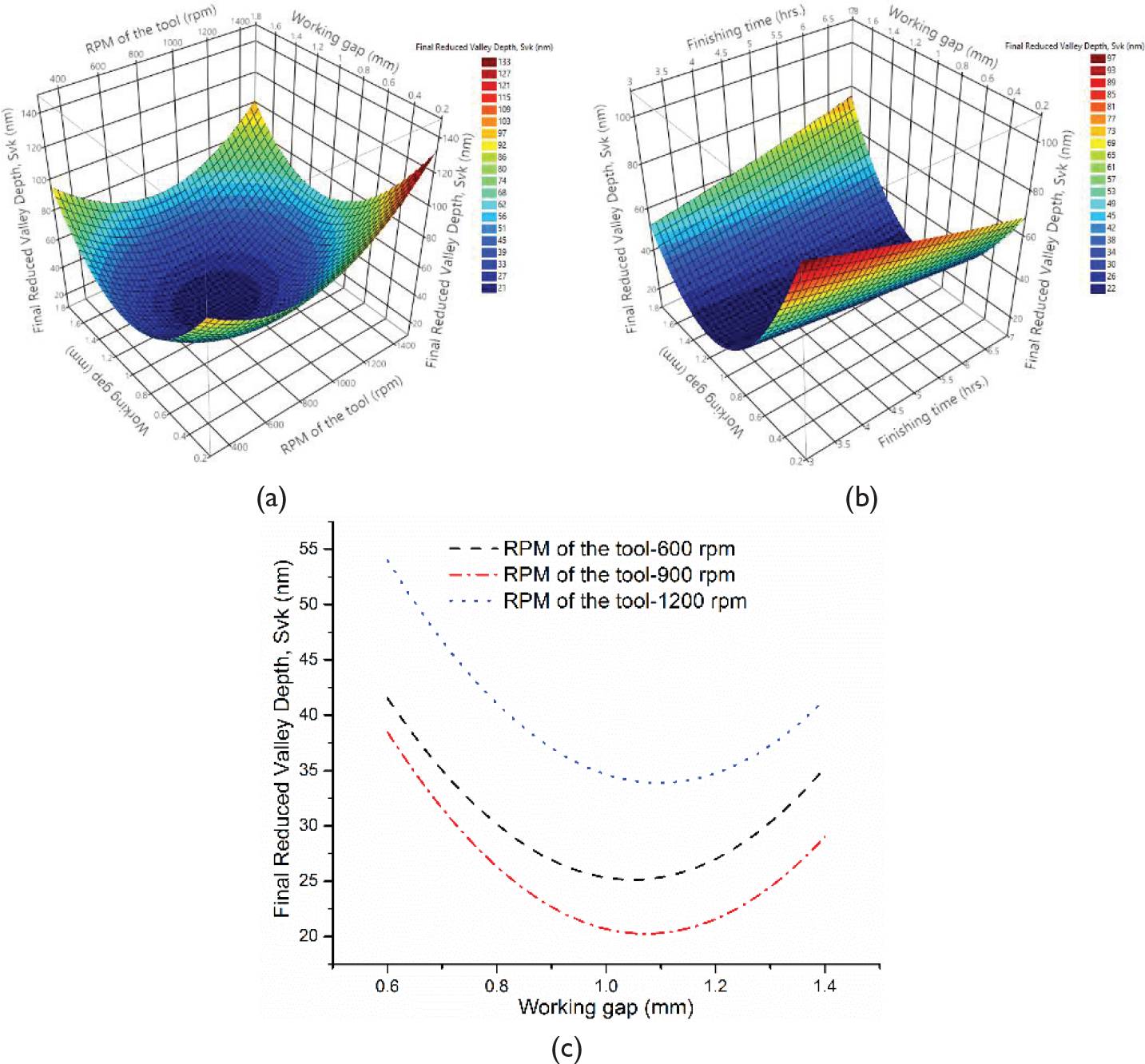
Figure 13(b) shows the effect of finishing time on final Svk values. Initially, with an increase in finishing time, the final Svk value starts to decrease. The increase in finishing time results in a better surface finish, which means reduction in valley depth. After 5.5 hrs, final Svk value starts to increase with an increase in finishing time. With a longer finishing time, the surface roughness increases resulting in deeper valleys. Hence, to achieve good Ti alloy implant performance rpm of the tool, working gap and finishing time should be in the range of 1100–1200 rpm, 0.6–0.8 mm and 5.5–6 hrs, respectively.

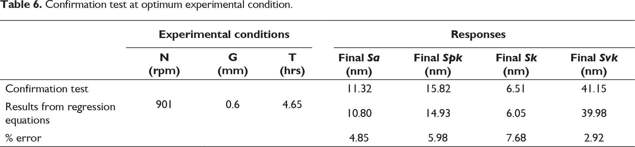
Confirmation tests

After conducting DOE, three confirmation tests are carried out at optimum process parameters (Table 5, Sol. no. 1). Average value of the 3D surface parameters from three confirmation tests is considered. Table 6 shows the responses from both confirmation test and the regression results at optimum experimental conditions, which shows close agreement between them. Also, the percentage error between them for all the 3D response parameters are less than 8%.

Table 5.

Results of the optimization study.

Sol. no.	N(rpm)	G(mm)	T(hrs)	Final Sa (nm)	Final Spk (nm)	Final Sk (nm)	Final Svk (nm)	Desirability
1	901.63	0.60	4.65	10.82	14.94	6.03	39.98	0.703	Selected
2	944.09	0.60	4.68	11.62	15.87	5.58	40.86	0.701
3	1,018.96	1.40	5.03	15.06	11.79	6.06	31.78	0.645

Table 6.

Confirmation test at optimum experimental condition.

	Experimental conditions			Responses
	N(rpm)	G(mm)	T(hrs)	Final Sa (nm)	Final Spk (nm)	Final Sk, (nm)	Final Svk (nm)
Confirmation test	901	0.6	4.65	11.32	15.82	6.51	41.15
Results from regression equations	901	0.6	4.65	10.80	14.93	6.05	39.98
% error				4.85	5.98	7.68	2.92

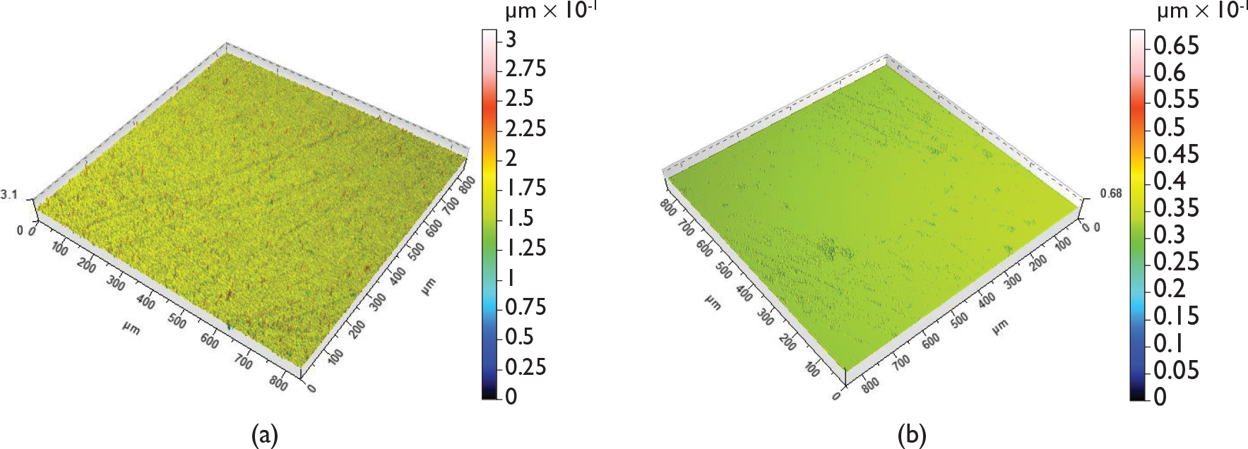
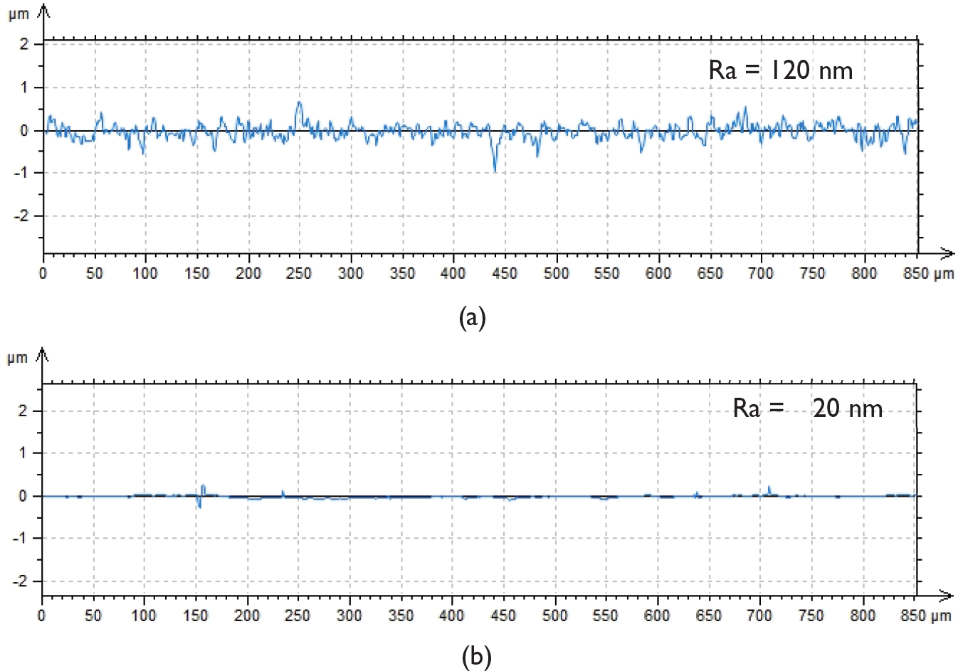
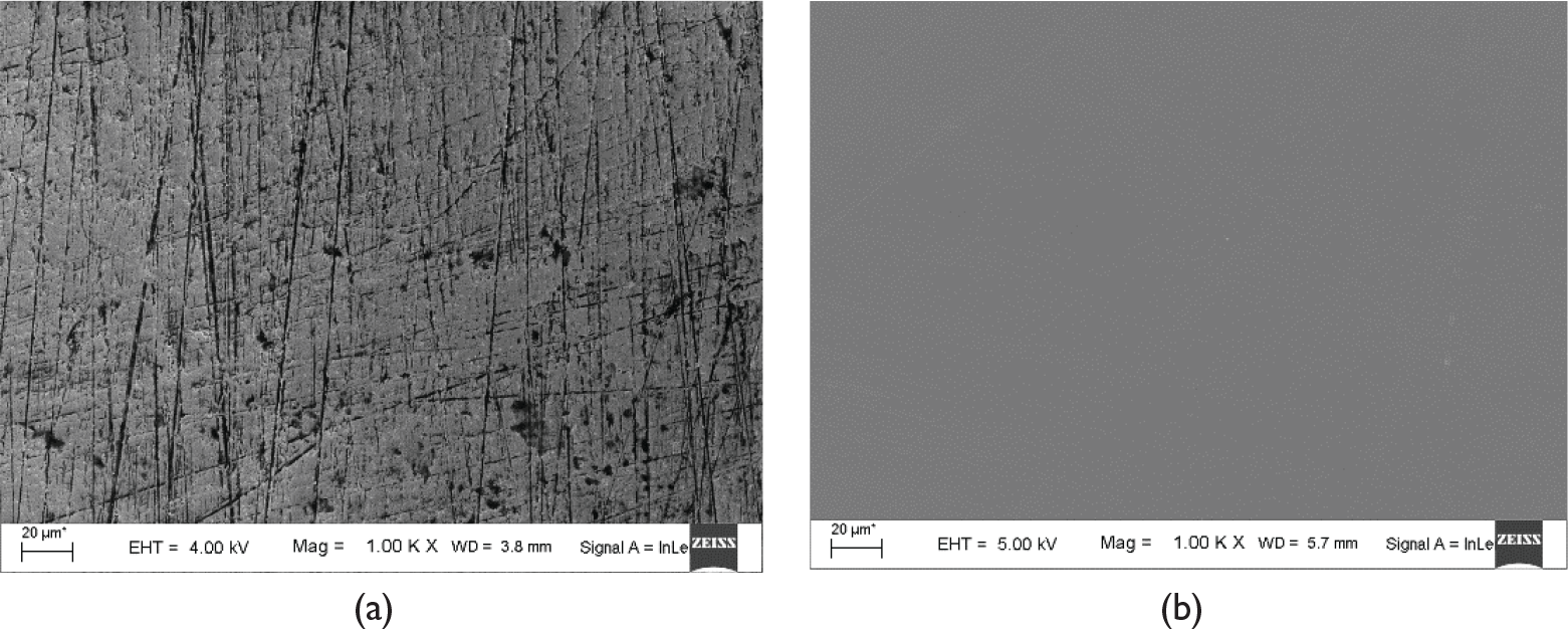
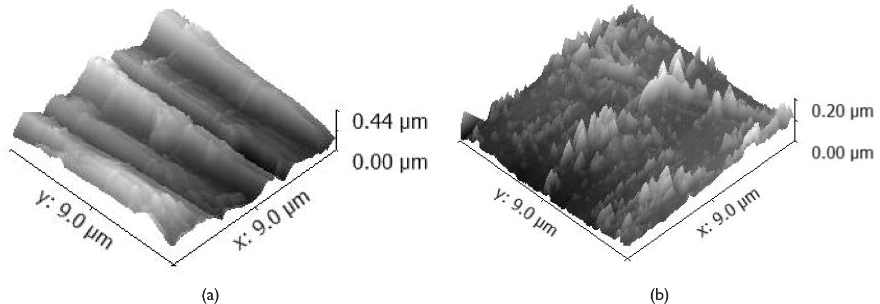
Surface roughness and surface topography of the finished components are analyzed using optical profilometer, FESEM and AFM. Figures 14(a) and (b) show the 3D surface topography of initial (before finishing) and final (after finishing) workpiece surfaces, respectively. The initial surface topography shows scratch marks as well as high peaks and deep valleys (Figure 14(a)). The finished surface shows reduced peak height and reduced valley depth (Figure 14(b)). Also, the smoothness of the surface is increased due to the finishing at nanometer level. Figures 15(a) and (b) show the initial and final surface roughness profiles of the workpiece, respectively. The initial surface roughness of the workpiece is 120 nm and it is reduced to very lower value of 20 nm in the final surface roughness profile. The percentage change in surface roughness is 83.33%, which proves that MFAF process is a very efficient finishing method to finish Ti alloy. Figures 16(a) and (b) show the FESEM images of the initial and final surface, respectively, at 1000X magnification. The FESEM image of the initial surface shows random scratch marks as well as deep valleys. The final surface is smooth and the scratch marks are reduced considerably as shown in Figure 16(b). Figures 17(a) and (b) show the AFM images of the initial and final surface topography, respectively. The final surface (Figure 17(b)) has reduced surface undulations than the initial surface (Figure 17(a)).

Figure 14.

3D surface topography of (a) initial (before finishing) and (b) final (after finishing) workpiece surfaces at optimum process parameters.

Figure 15.

2D surface roughness profiles of (a) initial and (b) final workpiece surface at optimum process parameters.

Figure 16.

FESEM images of (a) initial and (b) final workpiece surface at optimum process parameters.

Figure 17.

AFM images of (a) initial and (b) final workpiece surfaces at optimum process parameters.

Conclusions

The capability of the MFAF process to deliver implant worthy surface roughness and texture is analyzed here by exploring 3D surface roughness parameters. A DOE study consisting 20 experiments are conducted and the output responses are predicted using regressing analysis. After that, an optimization study is carried out to minimize the value of Sa, Spk and Sk and maximize Svk for achieving optimum implant surface roughness and surface topography. The optimum values of Sa, Spk,Sk, and Svk are observed as 901 rpm of the tool, 0.60-mm working gap and 4.30 hrs of finishing time. The optimized value of Sa, Spk,Sk, and Svk are 11.32 nm, 15.82 nm, 6.51 nm and 41.15 nm, respectively, and their values are more than sufficient against the requirement of the femoral knee joint implant surface. Hence, MFAF process provides nanometer-level surface finish along with the necessary surface topography for better wear properties to achieve better performance and longer implant life. From experimental analysis, it is observed that for good Sa values, the rpm of the tool, working gap and finishing time should be in the range of 800–1000 rpm, 0.8–1.2 mm and 4–5 hrs, respectively. For good Spk values, the rpm of the tool, working gap and finishing time should be in the range of 700–900 rpm, 0.9–1.2 mm and 4–5 hrs, respectively. For good Sk values, the rpm of the tool, working gap and finishing time should be in the range of 800–1100 rpm, 0.8–1.2 mm and 4.5–5.5 hrs, respectively. For good Svk values, the rpm of the tool, working gap and finishing time should be in the range of 1100–1200 rpm, 0.6–0.8 mm and 5.5–6 hrs, respectively. Hence, depending upon finishing requirements, the necessary values of the process parameters can be chosen to achieve required surface roughness and topography for implant surface. From experimental investigation, it is concluded that CIP chains break at a high rpm due to the shear thinning nature of MR fluid. Also, at high working gap, the finishing capability of abrasive particles reduces due to the insufficient magnetic field in the finishing zone. Furthermore, after 6 hrs of finishing time, the surface roughness of workpiece increases again due to the plowing of abrasive particle on already finished workpiece surface.

A final confirmation experiment is also conducted at optimized process parameter, which shows that the experimental results are nearly same as the predicted results obtained from regression equations. After measuring and comparing the surface topographies and roughness profiles of initial and final surface, it can be concluded that MFAF process provides nanometer-level finishing of Ti alloy with low peaks and shallow valley rather than initial surface.

Declaration of Conflicting Interests

The authors declared no potential conflicts of interest with res-pect to the research, authorship, and/or publication of this article.

Funding

We acknowledge Department of Science and Technology (DST), New Delhi, India, for their financial support for project no. SB/EMEQ-165/2013 entitled ‘Nanofinishing of Freeform Surfaces using Magnetorheological Fluid based Finishing (MRFF) process’.

References

Hryniewicz

Rokicki

Rokosz

Magnetoelectropolished titanium biomaterial. Biomater Sci Eng 2011; 227–247.

Wang

Yue

Bobyn

Surface characterization of metal-on-metal hip implants tested in a hip simulator. Wear 1999; 225: 708–715.

McGee

Howie

Costi

Implant retrieval studies of the wear and loosening of prosthetic joints: a review. Wear 2000; 241: 158–165.

Deltombe

Kubiak

Bigerelle

How to select the most relevant 3D roughness parameters of a surface. Scanning 2014; 36: 150–160.

Hilerio

Barrón

Vite

3D Characterization of surface state in a knee prosthesis. ASME World Tribol Congr World Tribol Congr III 2005; 2: 679–680.

Charlton

Blunt

Surface and form metrology of polished ‘freeform’ biological surfaces. Wear 2008; 264: 394–399.

Sarkar

Jain

Nanofinishing of freeform surfaces using abrasive flow finishing process. J Eng Manuf 2015; 1–15.

Sidpara

Jain

VK.

Rheological properties and their correlation with surface finish quality in MR fluid-based finishing process. Mach Sci Technol 2014; 18: 367–385.

Jain

VK.

Abrasive-based nano-finishing techniques: an overview. Mach Sci Technol 2008; 12: 257–294.

10.

Kordonski

Golini

Multiple application of magnetorheological effect in high precision finishing. J Intell Mater Syst Struct 2002; 13: 401–404.

11.

Shi

Dai

Peng

Magnetorheological finishing for high-precision optical surface. Opt Precis Eng 2009; 17: 1859–1864.

12.

Catrin

Taroux

Cormont

Efficiency of magnetorheological fluid finishing on the elimination of defects in fused silica optics. In: SPIE Optifab. International Society for Optics and Photonics, 2013, p. 88840A–88840A.

13.

Pollicove

Golini

Deterministic manufacturing processes for precision optical surfaces. Key Eng Mater 2003; 238–239: 53–58.

14.

Bedi

Singh

AK.

Development of magnetorheological fluid-based process for finishing of ferromagnetic cylindrical workpiece. Mach Sci Technol 2017; 1–27.

15.

Jung

Jang

K-I

Min

B-K

Magnetorheological finishing process for hard materials using sintered iron-CNT compound abrasives. Int J Mach Tools Manuf 2009; 49: 407–418.

16.

Han

Wang

Attempt at unitary magnetorheological finishing for a pierced die cavity. Proc Inst Mech Eng Part B J Eng Manuf 2010; 224: 879–886.

17.

Das

Jain

Ghoshdastidar

PS.

Nano-finishing of stainless-steel tubes using rotational magnetorheological abrasive flow finishing process. Mach Sci Technol 2010; 14: 365–389.

18.

Kumar

Jain

Sidpara

Nanofinishing of freeform surfaces (knee joint implant) by rotational-magnetorheological abrasive flow finishing (R-MRAFF) process. Precis Eng 2015; 42: 165–178.

19.

Sidpara

Jain

Nanofinishing of freeform surfaces of prosthetic knee joint implant. Proc Inst Mech Eng Part B J Eng Manuf 2012; 226: 1833–1846.

20.

Montgomery

DC.

Design and analysis of experiments. 8th ed. Wiley, 1976.

21.

Barman

Das

Design and fabrication of a novel polishing tool for finishing freeform surfaces in magnetic field assisted finishing (MFAF) process. Precis Eng 2017; 49: 61–68.

22.

Geels

Metallographic and materialographic specimen preparation, light microscopy, image analysis, and hardness testing. 15th ed. ASTM International, 2007.

23.

Sidpara

Jain

Experimental investigations into surface roughness and yield stress in magnetorheological fluid based nano-finishing process. Int J Precis Eng Manuf 2012; 13: 855–860.

24.

Derringer

Suich

Simultaneous optimization of several response variables. J Qual Technol 1980; 12: 214–219.

25.

Gregory

RD.

Classical mechanics . Cambridge: Cambridge University Press, 2006.

Magnetic field assisted finishing process for super-finished Ti alloy implant and its 3D surface characterization

Abstract

Abstract

Keywords

Introduction

(a) Surface roughness profile and (b) material ratio curve along evaluation length showing three functional parameters, that is, core roughness depth (Sk), reduced peak height (Spk) and reduced valley depth (Svk).

MFAF experimentation

(a) Magnetic field assisted finishing experimental setup, (b) novel developed tool and (c) measured magnetic flux density from tool-tip along line ab (Figure 2(b)).

(a) Schematic diagram of novel developed tool along with MR fluid and bio-titanium workpiece and (b) contour plot of magnetic field distribution during finishing.

MFAF tool along with MR fluid (a) before finishing and (b) during finishing with different forces (Fn: normal force and Fcfg: centrifugal force) responsible for finishing operation.

MR fluid chain formation (a) below and (b) at the edge of the novel developed tool.

(a) Toolpath and forces acting on active abrasive particle due to rotational and translational motions of the tool during finishing; surface profile of the component and normal and shear forces acting on abrasive particle (b) before and (c) after MFAF process.

Coded levels and actual values of the process parameters.

Plan of experiments.

Results and discussion

ANOVA for final Sa and final Spk.

ANOVA for final Sk and final Svk.

Effect of process parameters on output responses

CIP chains and abrasive particles in MR fluid below MFAF tool under (a) static condition, (b) nominal shearing condition and sheared chains without breaking and (c) high shearing condition and breaking of chains.

3D surface topography of workpieces: (a) before finishing, for (b) 1 mm and (c) 1.4-mm working gap with 1000 tool rpm and 4 hrs finishing time

3D surface topography of workpieces: (a) before finishing, after (b) 4.5 hrs and (c) 6 hrs finishing time with 1000 tool rpm and 1-mm working gap.

Effect of process parameters on final Sa

3D graph showing the combined effect of (a) rpm of the tool and working gap and (b) working gap and finishing time on final surface roughness (Sa); the effect of (c) rpm of the tool at different working gap and (d) working gap at different finishing time on final Sa.

Effect of process parameters on final Spk

3D graph showing the combined effect of (a) finishing time and rpm of the tool and (b) finishing time and working gap on final reduced peak height (Spk); the effect of (c) rpm of the tool and (d) finishing time on final Spk at different working gap.

Effect of process parameters on final Sk,

3D graph showing the combined effect of (a) rpm of the tool an d finishing time and (b) finishing time and working gap on final core roughness depth (Sk); the effect of (c) rpm of the tool at different finishing time on final Sk.

Effect of process parameters on final Svk

3D graph showing the combined effect of (a) working gap and rpm of the tool and (b) working gap and finishing time on final reduced valley depth (Svk); (c) the effect of working gap on final Svk at different rpm of the tool.

Confirmation tests

Results of the optimization study.

Confirmation test at optimum experimental condition.

3D surface topography of (a) initial (before finishing) and (b) final (after finishing) workpiece surfaces at optimum process parameters.

2D surface roughness profiles of (a) initial and (b) final workpiece surface at optimum process parameters.

FESEM images of (a) initial and (b) final workpiece surface at optimum process parameters.

AFM images of (a) initial and (b) final workpiece surfaces at optimum process parameters.

Conclusions

Declaration of Conflicting Interests

Funding

References

MFAF tool along with MR fluid (a) before finishing and (b) during finishing with different forces (F_n: normal force and F_cfg: centrifugal force) responsible for finishing operation.