
Abstract
In this article, we attempt to estimate the economic impacts of the US–China trade war that began in 2018. We used IDE-GSM, a computational general equilibrium simulation model, to estimate the economic impacts of a ‘full-confrontation’ scenario wherein both countries impose 25% additional tariffs on all goods imported from each other for 3 years 2019 onwards. In our calculation, the economic impact for the United States is −0.4% and −0.5% for China. Some Asian countries benefit from the trade war. As far as it remains bilateral, the trade war is only an issue for the concerned parties. We also ran the US–world trade war scenario, wherein the United States and all other countries impose a 25% additional tariff on all goods. The negative impact on the global economy is –0.8%, much more significant than the 0.1% impact from the US–China trade war. Thus, it is clear that the world cannot afford to engage in a multilateral trade war.
Introduction
On 5 December 2018, it was reported that US President Donald Trump and China’s President Xi Jinping agreed to temporarily pause further escalation of tariff rates on mutual imports for 90 days from 1 December 2018 onwards. During this period, both parties attempted to resolve various trade issues, including exchange rates and intellectual property rights, to avoid a full confrontation in the Group of Two (G2), namely, the United States and China, in the twenty-first century. As of the end of January 2019, the two parties have not reached an agreement to end the confrontation.
This trade war between the two countries began when President Trump imposed a 25% tariff on 818 Chinese goods valued at $34 billion effective 1 July 2018. China soon retaliated by imposing a 25% tariff on 545 US goods valued at $34 billion. Subsequently, the United States imposed a 25% tariff on an additional 279 Chinese products valued at 16 billion on 23 August 2018, and China immediately responded by imposing a 25% tariff on an additional 333 US products valued at $16 billion. On 24 September 2018, the United States imposed a third round of tariffs rated at 10% on $200 billion worth of Chinese products while China imposed a 5–10% tariff on $60 billion worth of goods from the United States.
It is unprecedented that the two biggest economies in the world have imposed import tariffs on each other on the global stage, clearly intending to harm the other. Numerous news articles have been published on this matter, most of which condemn both countries for damaging the global economy by discouraging world trade. However, the exact GDP loss of affected economies because of the US–China trade war that started in 2018 is not apparent.
In this article, we attempt to estimate the economic impacts of the US–China trade war on the global economy, especially on Asian economies, by using IDE-GSM, a computer simulation model based on spatial economics developed by IDE-JETRO. IDE-GSM is a computational general equilibrium model covering more than 160 countries at the national and subnational levels. It has been developed primarily to estimate the economic impacts of transport infrastructure, but it is also possible to estimate the impacts of tariff rate changes by using IDE-GSM. Estimating the economic impacts of the trade war by using IDE-GSM, we will evaluate an economic consequence through the trade channel, excluding political consequences and economic impacts through non-trade channels, such as a disturbance in the financial market and restrictions on technology transfer in high-tech sectors.
This article is structured as follows. First, we briefly introduce the simulation tool that we use—IDE-GSM. Second, we provide background information by describing the bilateral trade between the G2 countries and review some previous estimates on the trade war; we also propose a theoretical framework to analyse the trade war. Third, we construct a scenario for the trade war and present the estimated economic impacts using IDE-GSM, and then we analyse the simulation results and interpret them from a theoretical point of view. We also derive some policy implications from our analysis. The conclusion summarises the article and identifies issues for further research.
The Model
The Geographical Simulation Model, developed by IDE-JETRO (IDE-GSM), is a variation of the computable general equilibrium model based on spatial economics (Kumagai et al., 2013). IDE-GSM has been developed with two primary objectives: (a) to simulate the dynamics of the locations of populations and industries in East Asia over the long term and (b) to analyse the economic impacts of trade and transport facilitation measures (TTFMs), such as developing the transport infrastructure and reducing time and costs at national borders on regional economies at the subnational level. There are two endowments: labour, which is mobile within a country but prohibited from migrating to other countries, and land, which is unequally spread in all regions and is jointly owned by all the labour of each region.
The simulation procedures are as follows. First, according to the actual data set, with the given distribution of labour and regional GDP by sector and region, short-run equilibrium values 1 of nominal wages and price indices are obtained by iterative calculation. Observing the achieved short-run equilibrium, labour migrates among regions and industries, moving to the sector that offers higher nominal wage rates in the same region and to the region that offers higher real wages within the same country. This migration narrows the gap between nominal and real wage rates in a region and a country, respectively. Following these migration dynamics, we obtain a new distribution of labour and economic activities among regions and industries. We call this cycle of calculation ‘1 year’ in the simulation. With this new distribution and predicted national-level population growth given externally, the next short-run equilibrium is calculated for the following year, and we observe the migration dynamics again. These computations are repeated for 30 years, from 2010 to 2040.
IDE-GSM depends on two data sets. One is a geo-economic dataset, that is, economic and population data at the subnational level. We derive the regional-level GDP (RGDP) for the agriculture sector, mining sector, five manufacturing sectors and the service sector for 2010, primarily based on official statistics, sometimes utilising satellite imagery (Keola et al., 2015). The five manufacturing sectors are food processing, garments and textiles, electronics and electric (E&E), automotive, and other manufacturing.
These sectors behave differently in IDE-GSM. The agricultural and mining sectors are perfectly competitive and provide homogenous goods, using constant returns to scale technology. The manufacturing and service sectors produce many differentiated goods under monopolistic competition, using increasing returns to scale technologies. The agricultural and mining sectors use labour and land as inputs. The manufacturing sector uses labour and the intermediate goods produced by a firm in the same sub-sector of the manufacturing sector. The service sector uses labour as a sole input. Thus, the manufacturing sector has stronger agglomeration forces than the service sector does, and the service sector has stronger agglomeration forces than the agricultural sector does. The usage of land as an input in the agricultural and mining sectors leads to a stronger dispersion of forces than in other sectors.
The other dataset is a transport network dataset. The number of routes included in this dataset is more than 14,000 (land: 10,000, sea: 1,300, air: 2,150 and railway: 900). The route data consists of start city, end city, the distance between the cities, the speed of the vehicle running on the route, etc. The land routes between cities are primarily based on the ‘Asian Highway’ database of the United Nations Economic and Social Commission for Asia and the Pacific (UNESCAP), supplemented by the routes on various maps. The actual road distances between cities are used; if they are not available, the distances between cities in a straight line are employed.
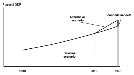
When we calculate the economic impacts of a specific TTFM, we take the differences in baseline and an alternative scenario (Figure 1). The baseline scenario incorporates infrastructure projects that were already completed by 2015. The alternative scenario assumes additional infrastructure development projects that are analysed in the simulation. We compare and show the differences between regional GDPs for each subnational region based on alternative scenarios against regional GDP for the same subnational region in baseline scenarios for a specific year. If a region under alternative scenarios has a higher (or lower) regional GDP (RGDP) than under the baseline scenario, we regard this surplus (or deficit) as a positive (or negative) economic impact of the TTFM.
In the baseline scenario, we assume a kind of business-as-usual situation. The following assumptions are maintained in all scenarios, including the baseline case, even if they are not specified in the following scenarios:
Each country’s national population is assumed to increase at the rate forecast by the United Nations Population Division until 2030. International labour migration is prohibited. Tariffs, non-tariff barriers and services barriers change as per free trade agreements (FTAs)/economic partnership agreements (EPAs) that are currently in effect and according to the phased-in tariff reduction schedule by the FTAs/EPAs and Hayakawa and Kimura (2015). The tariff revenue of each country is evenly distributed to the population of the country. We give different exogenous growth rates for each country’s technological parameters to replicate the GDP growth trend from 2010 to 2023, estimated and provided in the World Economic Outlook by the International Monetary Fund. After 2023, we gradually reduce the calibrated growth rates of technological parameters to half in 20 years.
Although TTFMs might have a negative effect on the regional economy under some simulation scenarios, it does not mean that the region is worse than the current situation. For instance, most Asian developing countries are expected to grow faster in the next few decades. Thus, the negative economic impacts from TTFMs offset only part of the gains from the expected economic growth.
Transport costs are of the iceberg type; if one unit of product is sent from one region to another, some portion of the unit melts, and a relatively smaller portion arrives. Depending on the ‘melted’ portion, the supplier needs to set a higher price. The increase in the supplier’s price compared to the producer’s price is regarded as the transport cost. Transport costs within the same region are considered negligible, and various trade costs are considered in IDE-GSM (Figure 2).
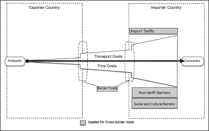
The sum of tariffs and non-tariff barriers (TNTBs) is estimated by employing the log odds ratio approach initiated by Head and Mayer (2000). We estimate industry-level TNTBs for 69 countries. TNTBs for the remaining sampled countries are obtained by prorating their TNTBs according to each country per capita GDP. To evaluate these estimates for TNTBs, we need the elasticity of substitution, the sources of which are explained below.
Next, we obtain NTBs by subtracting tariff rates from the TNTBs. Our data source for tariff rates is the World Integrated Trade Solution, particularly TRAINS (Trade Analysis and Information System) raw data. We aggregate the lowest tariff rates among all available tariff schemes at the tariff-line level into single tariff rates for each industry by taking a simple average for each trading pair. Available tariff schemes include multilateral FTAs and bilateral FTAs alongside other schemes such as the Generalised System of Preferences. Additionally, we consider the gradual tariff elimination schedule in six ASEAN + 1 FTA in addition to AFTA (ASEAN free trade area). We obtain information about whether each product finally attains a zero rate in ASEAN + 1 FTA from the FTA database developed in ERIA. We set the final rates for all products at zero in AFTA, owing to the lack of such information. Thus, we obtain different (bilateral) tariff rates and (importer-specific) NTBs by industry on a tariff-equivalent basis. Finally, our total transport costs are the product of the sum of physical transport and time costs and the sum of tariff rates and NTBs.
Parameters Specifying Each Industry.
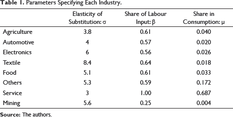
The consumption share of consumers by industry is uniformly determined for the entire region in the model. It would be more realistic to change the share as per country or region; however, this cannot be done because we lack sufficiently reliable consumption data. Each industry’s single labour input share is uniformly applied throughout the region and time in the model. Although it may differ among countries/regions and across time, we use an ‘average’ value; in this case, the value for Thailand, a country that is in the middle-stage of economic development and whose value is taken from the Asian International Input-Output Table for 2005 by the IDE-JETRO.
Background Information and Theoretical Framework of Trade War
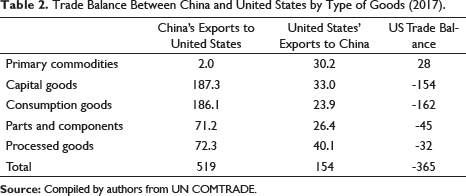
The United States and China are the two biggest economies in the world in terms of Nominal GDP in US dollar since 2010 and consist of 39% of world GDP in 2017. The United States is the biggest export market for China, consisting of 19% of total exports in 2017. China is the third-largest export market for the United States, following Canada and Mexico, consisting of 9% of total exports.
Trade Balance Between China and United States by Type of Goods (2017).
Spatial economics used in IDE-GSM will have two possibilities on the trade war’s consequence—higher tariffs between the United States and China. Two possibilities result from two different assumptions on the distribution of manufacturing firms and transport costs before the trade war.
As a thought experiment, we begin imagining the world as divided into three: the United States, China and the rest of the world. Transport costs are zero inside these three areas, yet firms incur transport costs between them. In this scenario, only the transport costs between the United States and China increased, while those between each of them and the rest of the world remain unchanged. However, transport costs between the United States and China are not significant enough to replace all direct trade between them into trade via the rest of the world.
Our manufacturing firms under this setting correspond to those in Puga and Venables (1997). Furthermore, Puga and Venables (1997) examined the impact of a preferential move toward a free trade area with two countries and reciprocal trade barriers between each of them and the remaining country unchanged. This change corresponds to the reverse case of our interest.
The first assumption is the symmetric distribution of economic activity among three regions at the initial stage. The second assumption is that the United States has the fewest manufacturing firms, and China has the most among the three at the initial stage. Furthermore, in the second assumption, the transport costs between the United States and China were lower than costs between each of them and the rest of the world before this trade war.
One of Puga and Venables (1997) results under the first assumption shows that the equilibrium number of firms decreases in the United States and China and increases in the rest of the world. These results mean that the manufacturing sector in the United States and China is likely to be negatively affected by the trade war, while the manufacturing sector in other countries is likely to be positively affected. This is the reverse case of ‘production shifting’ (Baldwin & Venables, 1995) that emerges because of regional economic integration. Consequently, the United States and China may be worse off and the rest of the world better off, which is one possibility of the trade war’s consequence.
Next, Puga and Venables (1997) numerical analysis under the second assumption shows that, if the transport costs between the United States and China surpass a threshold value, the roughly even distributions of firms and welfare among three locations emerge discontinuously. This is the other possibility of the trade war’s consequence.
Furthermore, the distribution of economic activity in the United States and China may change due to the high tariff rates between them. If the transport costs of the service sector decrease, the number of service sector workers in IDE-GSM will decrease in the city closer to the United States or China and increase in the inland city, as Matsuyama (2017) demonstrates. This tendency may strengthen the manufacturing sector due to the input-output linkage within each sub-sector in IDE-GSM.
There are some calculations on the US–China trade war. The National Institute of Social and Economic Research (NISER) calculated the economic impacts of the US–China trade war based on the simulation by NIESR’s Global Economic Model (Liadze, 2018). NISER estimated the economic impacts for three scenarios: 25% tariffs on $50 billion imports between each other, 10% tariffs on $200 billion US imports from China, and 10% tariffs on the remaining 25 billion US imports from China. The simulation assumes that these tariffs are applied for 3 years, and then they return to the initial levels. The economic impacts are proposed as percentages of GDP in the third year of the trade war. The economic impact for the United States in the worst scenario is around −0.8%, while that for China is slightly less than −0.8%, and the impact for the global economy is around −0.5% (Liadze, 2018). 2
The Daiwa Research Institute (DRI) also estimated the trade war’s economic impacts using the DIR macro model (Kobayashi & Hirono, 2018). It assumes that the United States imposes 25% tariffs on $50 billion imports from China and 10% tariffs on $200 billion imports from China. China then imposes 25% tariffs on $50 billion imports from the United States. DRI shows that the economic impacts are −0.15% for the United States and −0.14% for China, while the economic impact for Japan is −0.01% if some additional government expenditures from tariff revenues are not considered.
Furthermore, it is noteworthy that some factors affecting the actual economic impacts of the trade war are not included in this simulation analysis. These factors are as follows: (a) negative impacts from the uncertainty of US trade policy; (b) disturbance in the financial markets caused by the trade war; (c) negative psychological effects from the diplomatic tension between G2 countries; (d) an adjustment in the RMB/USD exchange rate, offsetting higher tariffs; (e) US policy on high-tech intellectual property rights that exclude certain Chinese companies from the US market; and (f) the indifference between multinational enterprises and local firms in IDE-GSM, which may soften the different impacts among countries.
The Scenario and Results
In this study, we formulate the US–China trade war as the case wherein both countries impose 25% tariffs on all the imports from each other. In other words, it is the trade war’s worst-case scenario. We assume that the tariffs remain the same during 2019–2021, and economic impacts are estimated at the end of 2021, compared to the baseline scenario. It must be noted that an additional government expenditure from tariff revenues for the United States and Chinese governments are not considered in the model.
Further, we ran another scenario: the trade war between the United States and the world, wherein we assume a 10% increase in bilateral tariff rates between the United States and all the other countries in the world. This scenario is intended at identifying the consequence if the United States applies its offensive trade policy against all other countries after China.
Economic Impacts of US–China Trade War (% of GDP in 2021, compared with the baseline).
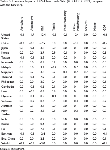
In the industrial sector, the biggest loser is the E&E sector in the G2 countries, which loses 12.4% in the United States and 7.5% in China. The automotive sector in the G2 countries is also negatively affected by the trade war, losing 0.8% in China and 1.7% in the United States. In contrast, the E&E sector in Japan, Singapore and Malaysia gain 3.6%, 3.6% and 3.3%, respectively.
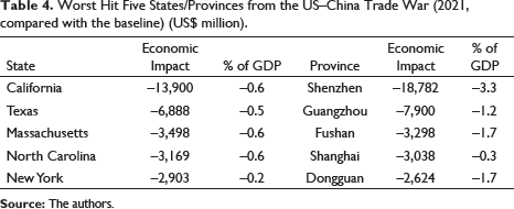
Worst Hit Five States/Provinces from the US–China Trade War (2021, compared with the baseline) (US$ million).
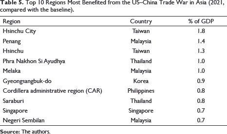
Top 10 Regions Most Benefited from the US–China Trade War in Asia (2021, compared with the baseline).
Top 10 Regions Most Benefited from the US–China Trade War in EU (2021, compared with the baseline).
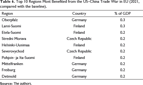
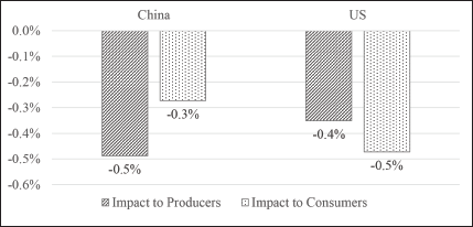
Figure 3 shows the economic impacts for the G2 countries concerning the GDP, which is evaluated from the production and consumption sides. The production (consumption) numbers are calculated upon each industry’s production (consumption) share when adjusting the GDP. For the production side, a more significant adverse economic impact is observed for China (−0.5%) than for the United States (−0.4%), while for the consumption side, a more significant adverse economic impact is observed for the United States (−0.5%) than China (−0.3%). This result is plausible, considering that most Chinese exports to the United States are consumed directly by consumers, as shown in Table 2.
Economic Impacts of US–World Trade War (percentage of GDP in 2021, compared with the baseline).
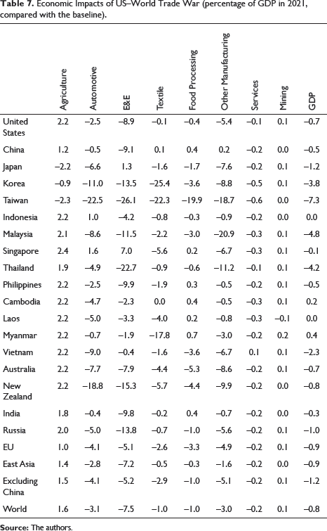
The countries that are most negatively affected by the US–world trade war is Taiwan (−7.3%), followed by Malaysia (−4.8%), Thailand (−4.2%) and Korea (−3.8%). The economic impacts from the US–world trade war for the 16 East Asian economies, excluding China, is −1.2%, which is much higher than the economic impact for China (−0.5%).
Analysis and Policy Implications
The simulation results revealed that economic impacts from the full-trade war between the G2 economies are significant for both countries. Negative impacts for the United States and China are −0.4% and −0.5% of their GDPs, respectively. Thus, considering that the IMF estimation of the GDP growth rates for the United States and China in 2021 are 1.7% and 6.0%, respectively, these negative impacts are significant for both countries. Furthermore, negative impacts to the E&E sector in the G2 countries are much more significant in terms of percentage, which loses 12.4% in the United States and 7.5% in China.
There are three possible factors that the E&E sector in the G2 countries has the largest negative impact from a 25% increase in the tariff rate. First, the tariff rate on E&E goods before the trade war is the lowest among the manufacturing sector for the United States and the second-lowest for China. This makes a 25% increase relatively large compared with the original tariff rate. Second, the transport costs of E&E goods are the lowest among the manufacturing goods because of a high price-to-weight ratio. This makes a 25% increase in the tariff rate relatively large compared with the total trade costs. Third, the elasticity of substitution parameter for E&E goods is relatively high among the manufacturing goods, making it easy to be substituted by imports from other countries.
It is noteworthy that our simulation predicts that the negative economic impacts for the United States are more significant for consumers than they are for producers, while for China, they are more significant for producers than for consumers. This difference may have some implications in the trade negotiation between the two countries. The US government is more likely to be criticised by the public for increased consumer product prices.
In contrast, the economic impacts for the global economy are not significant, that is, 0.1% of the total GDP. Our simulation results revealed that the trade war between G2 itself is not likely to trigger another deep recession for the global economy because most of the negative impacts remain within the two parties involved in the trade war. It is not surprising that a bilateral trade war primarily harms the countries involved.
Our simulation results predict that some countries benefit from the trade war because of the trade diversion effects. Theoretically, a bilateral trade war—a mutual increase in bilateral trade costs—works just like the reverse of a bilateral FTA—a mutual reduction in bilateral trade costs. It is also well known that a bilateral FTA has trade diversion effects, which harms third-party countries. By contrast, a bilateral trade war is likely to cause reverse trade diversion effects, which benefits third-party countries.
Seventy per cent of US firms in southern China refrain from any further investment in China and are planning to relocate their production to other countries (Wong, 2018). The Economist Intelligent Unit (EIU) published a list of ‘winners’ of the trade war by industry. Malaysia and Vietnam are nominated as the winners with strong benefits in the information and communications technology sector, while Bangladesh, Vietnam and India are nominated as the winners with strong benefits in the readymade garments sector. For the automotive sector, Malaysia and Thailand are nominated as the winners with strong benefits (EIU, 2018). Thus, the EIU predictions are mostly in line with our simulation results.
On the contrary, if the United States tries to apply its offensive trade policy for other countries following China, its negative impacts on the global economy would be significant. Some small and medium Asian economies—such as Taiwan, Korea and some ASEAN member countries—cannot afford to confront the trade war against the United States because they are too dependent on the US market for their exports. This scenario becomes less likely as President Trump left office by the end of 2020. Still, there is a possibility of ‘decoupling’ supply chains between US-friendly countries and China-friendly countries, which could pose a greater risk to the global economy.
Conclusions
In conclusion, we estimated the economic impacts of the US–China trade war through the trade channel using IDE-GSM. Accordingly, a few publications have revealed numerical economic impacts from the trade war thus far, not only for the United States and China but also for other countries. Thus, this study will be valuable for researchers as well as for policy- and decision-makers.
Considering only economic impacts through trade channels, the trade war is harmful to both the United States and China, although it is not likely to lead the global economy to a severe recession. It is practically inappropriate to brand the trade war as the primary cause of a potential slowdown in the G2 countries and/or the global economy without conducting any calculations based on economic models.
Some industries in some countries may benefit from the trade war owing to the trade diversion effect. News reports are stating that some firms have changed their procurement from China/the United States to other countries for exports to China/the United States. However, this potential benefit to other countries is not likely to be fully explored because it is highly uncertain how much longer this trade war will continue.
As far as the trade war remains bilateral, it is an issue only for the concerned parties. However, it will be a completely different scenario if the trade war would involve third-party countries. With the departure of President Trump, the scenario of the United States unilaterally raising import tariffs is no longer realistic, but on the other hand, the ‘decoupling’ of supply chains between the United States and China poses a significant risk to the global economy. This ‘decoupling’ scenario should also be investigated in detail in future research.
Footnotes
Acknowledgement
Authors are grateful to two anonymous referees of the journal for their useful comments. Views are authors’ own. Usual disclaimers apply.
Declaration of Conflicting Interests
Funding
The authors received no financial support for the research, authorship and/or publication of this article.