






Abstract
Simulation–optimization is often used in enterprise decision-making processes, both operational and tactical. This paper proposes a data-driven, declarative approach to enterprise optimization. In our generic simulation–optimization approach, a declarative constraint satisfaction problem (CSP) is automatically customized given a simulation model and a problem instance. We construct the declarative model by training a neural network on the simulation model and embedding the trained network in the CSP. The approach allows the embedding of a wide variety of complex problems, is able to handle multi-objective problems, is flexible to changing multiple objectives simultaneously, and allows the modeler to focus on what problem needs to be solved by a computer instead of how the computer should solve it. We demonstrate the value of this neuro-symbolic approach in experiments on two problem domains. Furthermore, we show how low discrepancy sampling, weighted composite objectives, and linear activation functions can improve the performance of neural embeddings in CSP.
Introduction
Managerial decisions are often an attempt at balancing multiple objectives, when critical decision factors are unclear and causal effects are hard to explain (Tan et al., 2020). Hence, decision makers (DMs) tend to use various tools, such as simulation, to gain insight into how an enterprise might behave in complex or future scenarios (Kampik and Najjar, 2019; Vernadat, 2020). With simulation, various managerial interventions can be analyzed for the likely outcomes. DMs that use simulation models in practice are often interested in finding “optimal” inputs with respect to an observed “problem”—an undesired property of the system that can be tackled by taking intervening action (Bock et al., 2018; Laguna and Marklund, 2013).
Finding these inputs by exhaustively trying out them all through simulation is feasible with only limited success on complex simulation processes, for the number of possible inputs grows exponentially with respect to the number of input parameters (Laguna and Marklund, 2013). On the other hand, using a pure optimization model to compute the “optimal” inputs—that is, omitting simulation—can be incapable of capturing all complexities and dynamics of a system (Laguna and Marklund, 2013). Hence simulation–optimization (SO) seeks to combine the benefits of both by using simulation to represent the actual system and optimization to find optimal simulation inputs (Teerasoponpong and Sopadang, 2021), for example, to determine strategic marketing decisions (Schlosser et al., 2019).
This article situates enterprise optimization (Grossmann, 2014) as optimization—that is, forming strategies to obtain some outcome—put in the context of managing an enterprise. A wide variety of enterprise optimization strategies and tools exist, for which an overview can be found in Varma et al. (2007).
A mapping from problem description to a formal SO model is non-trivial. From a modeler’s perspective, existing enterprise modeling (EM) methods offer only tenuous concepts of “problems” (Bock et al., 2018). From a computational perspective, optimization models can be difficult for a DM with a non-technical background to understand when the model is heavy with formal mathematics.
A path to model problems in a more understandable but computer-parseable format is with constraint programming (CP; Andringa and Yorke-Smith, 2021). CP is a declarative paradigm for defining combinatorial optimization; it allows one to describe diverse real-world problems through constraints, that is, statements which pose some relation among the problem’s variables (Rossi, 2000). Notably, the expressiveness of CP means its formal models can be more human-like than, for instance, mixed integer programming optimization models.
This article addresses the modeling challenge of SO for the enterprise by means of CP and automated modeling. The simulation model is represented by a “model of a model,” that is, meta-model (Jin et al., 2001). Meta-modeling techniques range from descriptive representations of ontological concepts to algorithms to make faster approximations of complex computer code (Atkinson and Kuhne, 2003; Jin et al., 2001). We focus on the latter by representing the simulation model with a neural network (NN). NNs are capable of learning behavior of complex systems and require little engineering by hand, making them applicable in many domains (Bartolini et al., 2011; LeCun et al., 2015; Teerasoponpong and Sopadang, 2021). Our approach is to train an NN on simulation data and automatically embed the NN into the CP model; we then solve multiple sampled instances of the CP model to obtain an approximation of the corresponding pareto frontier of the underlying enterprise optimization problem.
We argue that embedding an NN into a declarative model adds additional flexibility during the problem-solving process, since a change of objective can be evaluated without making additional simulation calls. This flexibility can be desirable in various situations, for example, when: The DM does not know all specifications of the problem it wants to solve (e.g., information by a third party is required), but does know how the system currently behaves, and would like to make preparations such that problems can be solved on-the-go without making computationally expensive simulation calls. The DM has a large collection of problems that needs to be solved, making setting up a separate feedback loop for every problem infeasible. The DM is not able to do simulation during the problem-solving phase.
We argue that the proposed methodology can be applied to a wide range of problems due to its generality. The two main components of the approach—CP and machine learning—are both effective in modeling complexity. CP is able to model complex problem structures, whereas (deep) machine learning is able to capture complex relationships between variables.
A preliminary report of this work appeared at a conference (Andringa and Yorke-Smith, 2021). That initial paper showed how easy-to-understand CP programs can be constructed from descriptive problem descriptions and how these can be evaluated to make strategic decisions. In this full article, we further detail the approach and particularly improve performance and show generality: The use of low discrepancy sampling to determine what weights to set to objectives, to obtain higher quality problem instances. The use of various output activation functions in the trained network, for more efficient constraint satisfaction problem (CSP) embeddings of the network. The direct optimization toward a composite weighted objective instead of considering thresholds. More detailed computational experiments and experiments on a new problem domain.
The remainder of the article is structured as follows. Section 2 discusses relevant literature, approaches, and techniques. Section 3 discusses our approach in more detail. Section 4 shows the applicability and performance of the approach through a set of experiments and discusses the results. Section 5 concludes with a discussion of future work.
Constraint Programming (CP)
CP is an expressive yet practical approach to optimization, used in a wide variety of applications (Rossi, 2000; Wallace, 2020). It solves constraint satisfaction problems, which consist of a set of variables, each with a domain of permitted values, and a set of constraints specified in a logical formalism. A solution to a CSP is an assignment of a value to every variable from its domain, such that all the constraints are satisfied. Soft CSPs permit the constraints to be satisfied to a degree, rather than binary satisfaction. Constraint optimization problems (COPs) include an objective function. For both CSP and COPs, the resulting model is passed to a (black-box) solving algorithm. A wide variety of such solvers, complete and incomplete, are available, such as or-tools from Google (Perron and Furnon, 0000).
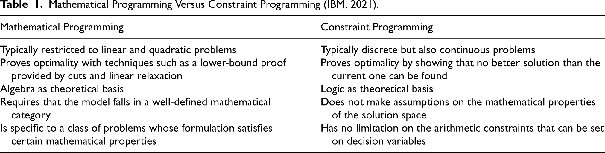
A common optimization methodology is mathematical programming (MP), archetypally mixed integer linear programming. Although CP and MP share a similar model-and-solve paradigm—there is a set of decision variables, a set of constraints, and often an objective function to maximize or minimize—CP is a more expressive formalism. It can be thought of as a generalization of mixed integer programming to non-linear and non-arithmetic constraints (Wallace, 2020). Table 1 provides an overview of the differences between CP and MP. Notably for the purpose of this article, the expressive nature of CP allows for models which are closer to human-level expression of problems (Buscemi and Montanari, 2008).
Mathematical Programming Versus Constraint Programming (IBM, 2021).
Mathematical Programming Versus Constraint Programming (IBM, 2021).
In our preliminary work, we set weights for the objectives in the composite objective (see Section 3 for more details) through uniform random sampling. As an alternative approach, we consider Quasi-Monte Carlo sampling. Quasi-Monte Carlo is attained by using quasi-random—also called low-discrepancy—sequences in Monte Carlo sampling (Caflisch, 1998). Low discrepancy sequences aim to sample a number of points that efficiently uniformly cover some
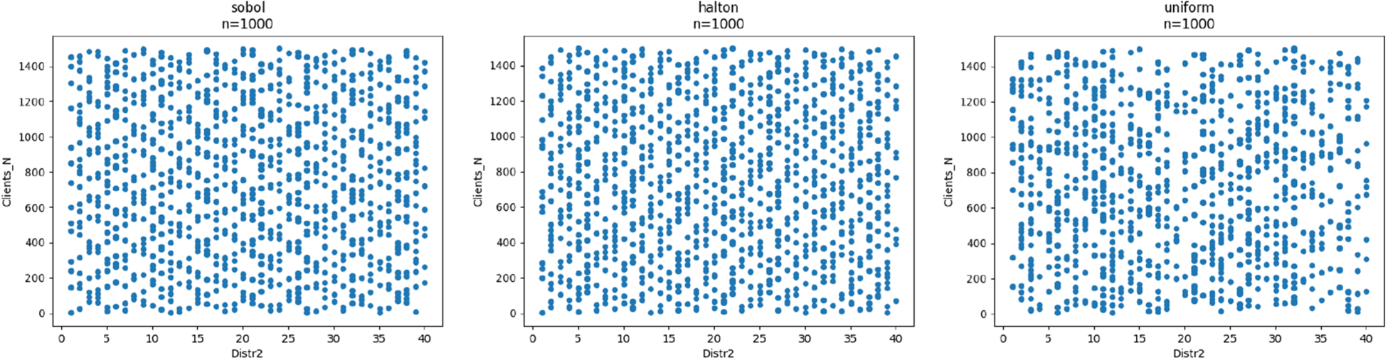
Demonstration of two low-discrepancy sampling methods (Sobol and Halton) as opposed to uniform sampling for 1,000 data points. The plot visualizes how both low-discrepancy sequences have less gaps and clusters.
As discussed in the introduction, the technique described in this article falls under the category of simulation–optimization. More specifically, a function–estimation-based approach, where an NN is fitted on the underlying system.
The literature on SO tends to favor evolutionary search to find optimal simulation inputs (Laguna and Marklund, 2013; Teerasoponpong and Sopadang, 2021; Yalcin et al., 2022). This black-box SO approach can be convenient when a quick evaluation of the simulation model is possible. However, if simulation is expensive—frequently the case with simulators—advanced techniques are necessary to limit the number of simulation calls (Lombardi et al., 2017).
Instead, we adopt an empirical decision model learning (EML; Lombardi et al., 2017), which differs in various ways from black-box optimization as shown in Table 2. EML is a methodology that learns relations between decidables (controllable variables) and observables (uncontrollable parameters) from data, and encapsulates these relations into components of an optimization model. Data can be harvested from a real system or a predictive model, such as a simulator. The encapsulation can be done by machine learning methods, for example, an NN.
Black Box Optimization Versus Empirical Model Learning (Lombardi et al., 2017).

Black Box Optimization Versus Empirical Model Learning (Lombardi et al., 2017).
Combining CP with EM is recognized as valuable in the literature. Several studies couple CP with the closely-to-EM-related Business Process Management to solve (complex) scheduling and planning problems, as the declarative paradigm allows them to conveniently embed their custom constraints (Jimenez-Ramirez et al., 2012; Wiśniewski et al., 2021). However, these studies typically require the DM to describe the flow of the system in the CP model. In contrast, this article considers a more general approach and studies CP models that merely describe the problem to solve. The DM is therefore not required to describe how the system operates. Differently stated, the DM can treat the simulation model as a black box and can focus on describing what relation between simulation inputs and outputs should be satisfied. It does not have to consider details of internal processes, as these are modeled by means of a simulation model. We believe these black-box properties make the approach applicable to a wide variety of problems, since the only requirement is access to a simulation model and a problem that can be defined with CP, given the simulation inputs and outputs.
Methodology
Figure 2 provides an overview of our approach. It has two main characteristics. First, we use simple—understandable for those with a non-technical background—CP to model the problem. Second, we represent the simulation model automatically in an optimization model by representing it as an NN. This section details the two main components of our approach. Then, multiple objectives and the solving procedure are discussed.
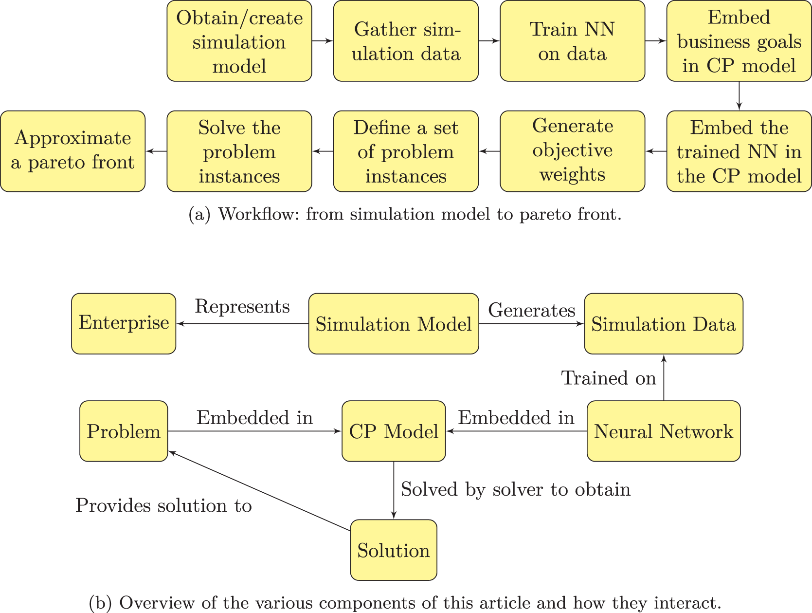
Approach summarized. A simple NN is trained on simulation data. Next, business goals and trained NNs are embedded in the CP model. By utilizing soft constraints and various weight and threshold parameters, an approximation of the Pareto front for the various objectives is formed. (a) Workflow: from simulation model to Pareto front. (b) Overview of the various components of this article and how they interact. Note. NN = neural network; CP = constraint programming.
In this article, the simulation model is assumed to represent a complex real-world system. It can, for example, be derived from an enterprise model (Vernadat, 2020). How to design a qualitative simulation model is not in the scope of this article: the reader is referred to Kampik and Najjar (2019) and Laguna and Marklund (Laguna and Marklund, 2013).
The first main component is a meta-model, derived from a simulation model representing the behavior of a system. This allows the DM to consult the meta-model instead of the simulation, such that simulation calls do not have to be made during the solving procedure. Deriving such a meta-model poses a tradeoff. On the one hand, it should reflect the simulation model properly. On the other hand, it should be convenient enough to allow optimization. This dilemma corresponds with a fundamental computational reality, namely the tradeoff between expressiveness and tractability. A model should be detailed enough such that it makes sense—it is expressive—but not too detailed because otherwise computations cannot be made feasibly—it lacks tractability (Brachman and Levesque, 2004). This article proposes using NNs as meta-models for several reasons: NNs are able to learn behavior of opaque or very complex systems, without requiring detailed knowledge of their components and interactions (Bartolini et al., 2011; LeCun et al., 2015). They are capable of dealing with both the non-linearity and uncertainty of the underlying system (Teerasoponpong and Sopadang, 2021). NN embeddings in optimization models have shown good performance in comparison to other combinations of optimization methods with machine learning techniques (Lombardi et al., 2017). Compared to other machine learning techniques, NNs are very capable in identifying what features are interesting and excel at handling high-dimensional input data. The result is that NNs require very little engineering by hand and are applicable in many domains (LeCun et al., 2015).
The activation functions also play a crucial role in NN (Dubey et al., 2021). A wide variety of activation functions exist, such as polynomial, adaptive, and rectified linear unit-based functions. For a comprehensive survey and benchmark study on activation functions, we refer to Dubey et al. (2021). The logistic sigmoid activation function is a popular and traditional non-linear activation function:

Using a convex activation function allows solvers to solve by means of convex optimization, which tends to converge to a solution much faster than non-convex optimization (Nesterov and Nemirovskii, 1994). Although sigmoid tends to perform very well for many deep learning applications, it includes an exponential quadratic term, which has a major impact on the solving time as it introduces non-linearity. Alternatively, one could consider activation functions that are linear—while retaining properties that are often found in non-linear activation functions—and might thus be more fitting for a CP embedding.
For this reason, in this article, we study the performance of two alternative approaches to the sigmoid activation function. The first is a quadratic variant power2, which replaces the 
The second is a semi-linear variant taylor1, based on the first term of the Taylor approximation of the sigmoid function:

Figure 3 visualizes the shape of the discussed functions. It shows all three are non-linear, which is an often desired property of activation functions (Dubey et al., 2021). It is noteworthy that the sigmoid is the only injective function: no output can be achieved in multiple ways. Our experiments will examine the tradeoff between the linearity of power2 and taylor1 versus the injective sigmoid.
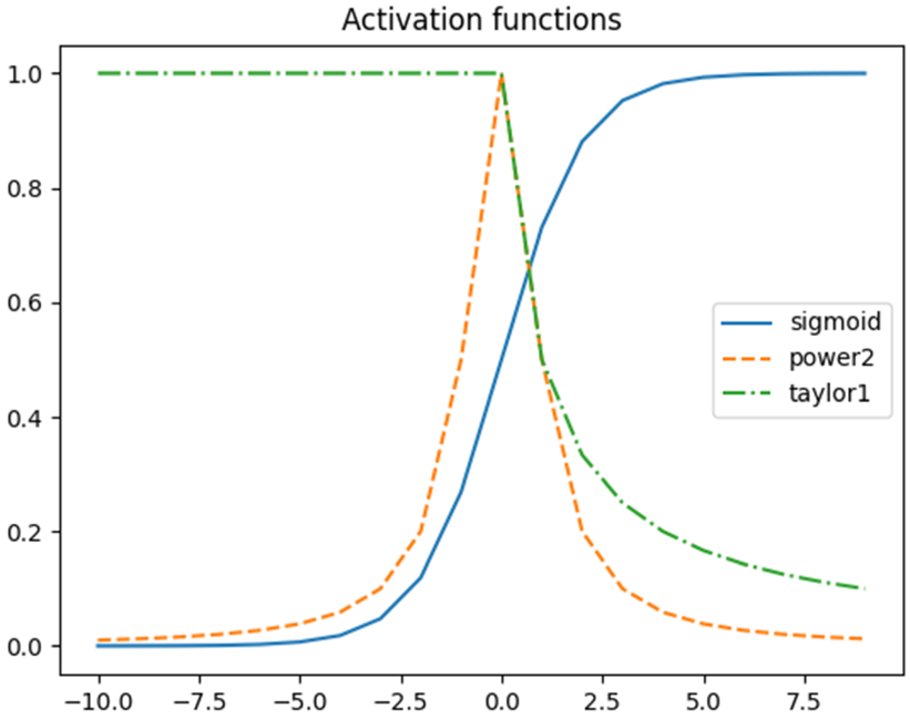
The shape of three activation functions.
Besides the NN, the second main component we need is the CP model. It intends to represent a problem to be solved. There are three main aspects to be identified in problems, namely (1) an as-is enterprise optimization scenario which is considered to be non-optimal, (2) uncertainty about what decision would lead to the preferred situation, and(3) a preferred situation to achieve (Bock et al., 2018). We construct the CP model accordingly: The current situation is modeled by a simulation model and represented by a trained NN. An NN can be embedded into a CP model, which allows expressing constraints over the NN output (Bartolini et al., 2011). Uncertainty is also incorporated by the NN. Training an NN creates a predictive model. In other words, the NN is used to tackle the uncertainty involved in the problem by giving insight into the correlation between variables and parameters in the decision model. The preferred situation is incorporated by the objective function. In our approach, the objective function is expressed by composite weighted objectives.
It is reasonable to believe most—if not all—problems can be described by elements also found in CP. This is based on the theoretical conceptualization of a problem by a meta-model presented in Bock et al. (2018), where the concept of a problem is decomposed. The interconnection between this decomposition and CP is shown in Table 3.
Concepts From the Meta-Model Presented by Bock et al. (2018) and Their CP Equivalents.
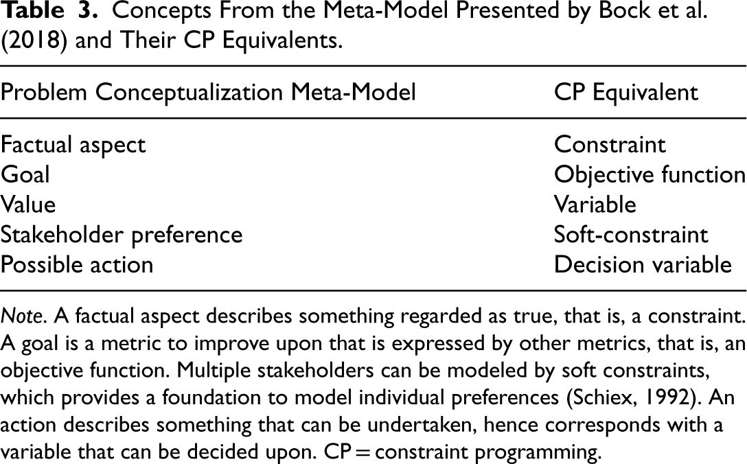
Note. A factual aspect describes something regarded as true, that is, a constraint. A goal is a metric to improve upon that is expressed by other metrics, that is, an objective function. Multiple stakeholders can be modeled by soft constraints, which provides a foundation to model individual preferences (Schiex, 1992). An action describes something that can be undertaken, hence corresponds with a variable that can be decided upon. CP = constraint programming.
As noted in Section 2, constraints expressed in natural language can be formalized in CP at a higher level compared to other optimization methods. The result is that constraints expressed by the DM describing what solution it aims to seek can be conveniently expressed in the CP model. For example, CP makes it convenient to state some relationship between variables that should always be satisfied, such as “machine A should never produce more than machine B” or “department C should always have more employees than department D”; so-called global constraints are particularly useful (Wallace, 2020). Figure 1 shows an example CP model that highlights its readability. We use the modeling language MiniZinc; MiniZinc conveniently connects to various solvers (Nethercote et al., 2007).

Our approach embeds an NN into a CP model by expressing the value of a node as a function of the values of nodes in a previous layer. This is based on the concept of neuron constraints, which allow one to encode complex networks using a limited number of basic components (Bartolini et al., 2011). An example of such an embedding can be found in Appendix B.
So far, we have a CP declarative model with an embedded NN. We next discuss how to obtain solutions, and moreover, what kind of solutions are to be sought.
Most methods on multi-objective decision making in business analytics are posteriori, in the sense that they obtain preference information—how much each objective is preferred over the others—from the DM after computing solutions (Yalcin et al., 2022). These methods are useful when the DM is interested in the scope of actions she can take—particularly useful when there is no single dominating solution—as multiple solutions are provided instead of a single one. In CP, preference information is the input, since the CP model is asked what inputs are necessary to satisfy certain objectives. As such, the approach can be made posteriori by evaluating a set of problems covering the variety of possible preferences.
We put our focus on approaches that do not require preference information beforehand. In our preliminary report (Andringa and Yorke-Smith, 2021), this was realized by a possibilistic CSP, where each objective had a corresponding weighted soft constraint (WSC; Schiex, 1992). A WSC has a weight, indicating the importance of its being satisfied, and a threshold. For a maximization objective, the WSC is satisfied if the objective value exceeds the threshold, and for a minimization objective if it does not. Then, random weights and thresholds are generated in order to create a set of problem instances. Next, this set of problems is solved. Their dominating solutions form the output.
For the experiments in this article, we considered to optimize toward weighted composite objectives, that is, we do not specify thresholds as the objective function equals a scaled sum of the objectives. The main motivation for a preference over this “direct” approach of the possibilistic CSP is, as the name already states, a more direct representation of the goal in this experiment, namely converging toward a Pareto front. This makes it easier to understand and construct the CP models, as it does not require a threshold parameter.
For problems that need to preserve the binary pass/fail properties of the problem, a possibilistic CSP approach might be more fitting. A trivial example is when the DM is interested in optimizing some target value
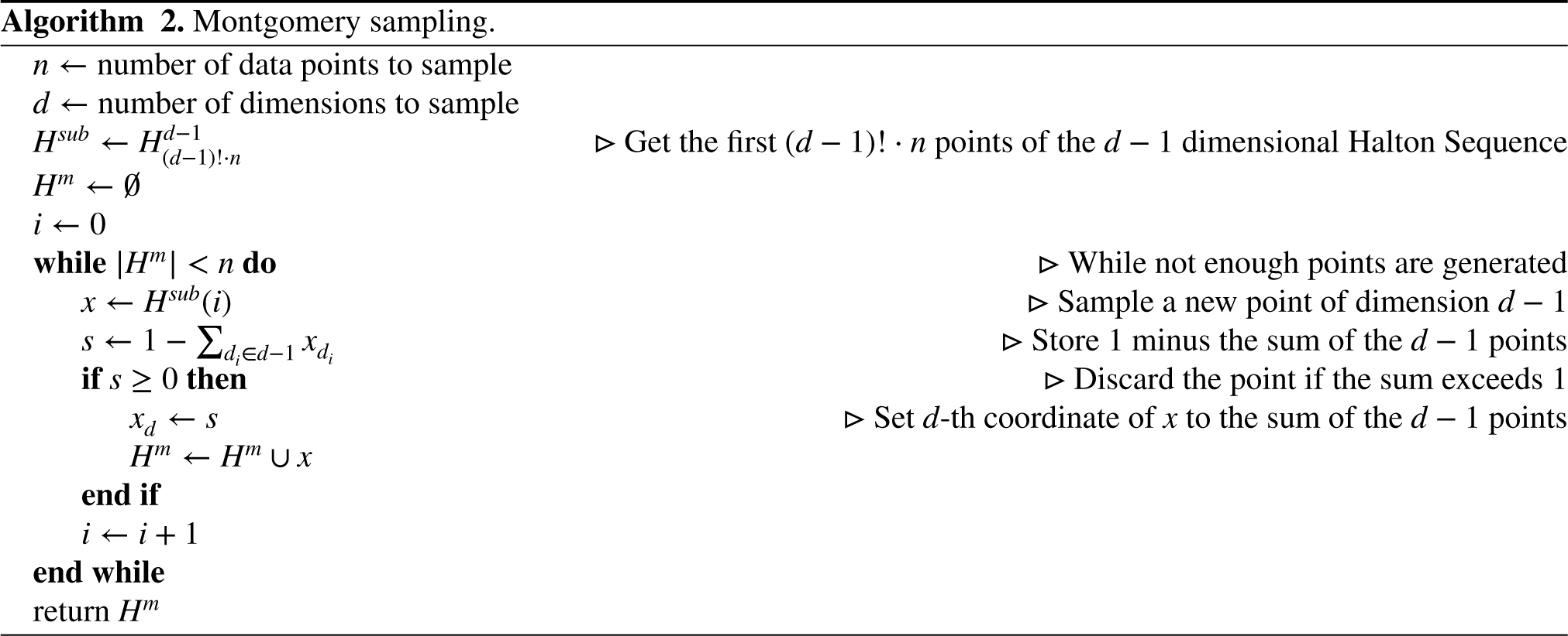
Furthermore, instead of generating the weights for individual objectives in the composite objective uniformly at random, we consider generating these by deterministic low-discrepancy sequences. The idea is that this improves the quality of the Pareto front, as the generated CSP instances are more evenly spread in the objective space. Since the sum of the sampled weights should sum to one, this article considers Montgomery sampling (see Algorithm 2), a variant on low-discrepancy sampling. Montgomery sampling takes a
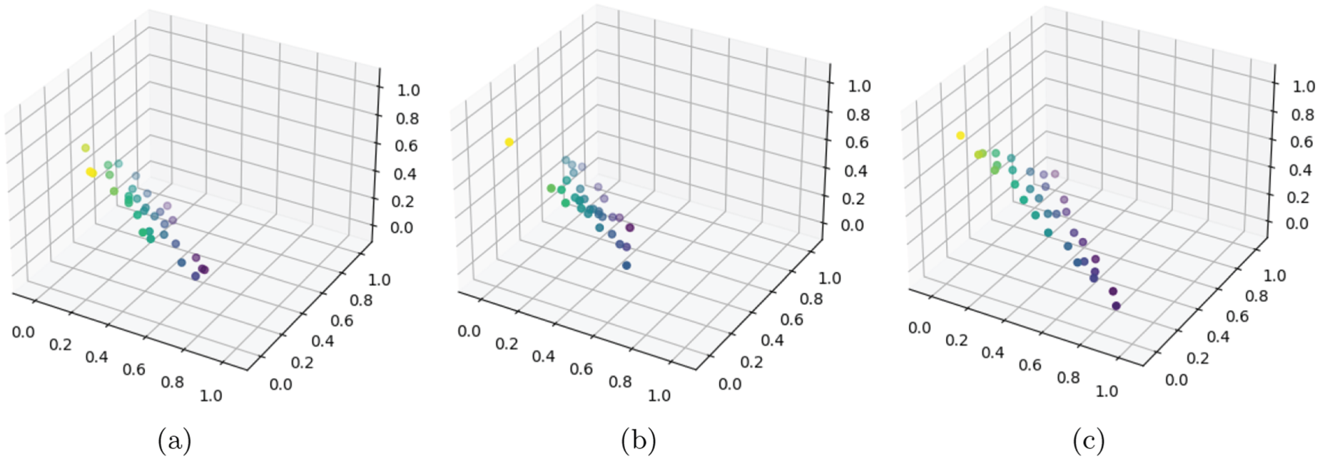
3D plots to show the effects of Montgomery sampling compared to uniformly sampling and a normalized Halton sampling. 32 three-dimensional data points were generated. The two normalized variants were implemented by first generating the points according to their underlying sequence, and then for each point, dividing each of its value by the sum of its values such that the summation constraint was satisfied. Montgomery sampling tends to outperform the other two in terms of L2* discrepancy (Zhou et al., 2013). Visually, this can also be observed, as the triangle-shaped solution space is more easily noticeable for Montgomery sampling than for the other two methods. (a) Normalized Halton L2* discrepancy = 0.135. (b) Normalized Uniform L2* discrepancy = 0.155. (c) Montgomery L2* discrepancy = 0.119.
It should be noted that Sobol and Halting sampling sequences tend to become infeasible to compute for higher dimensions (around approximately
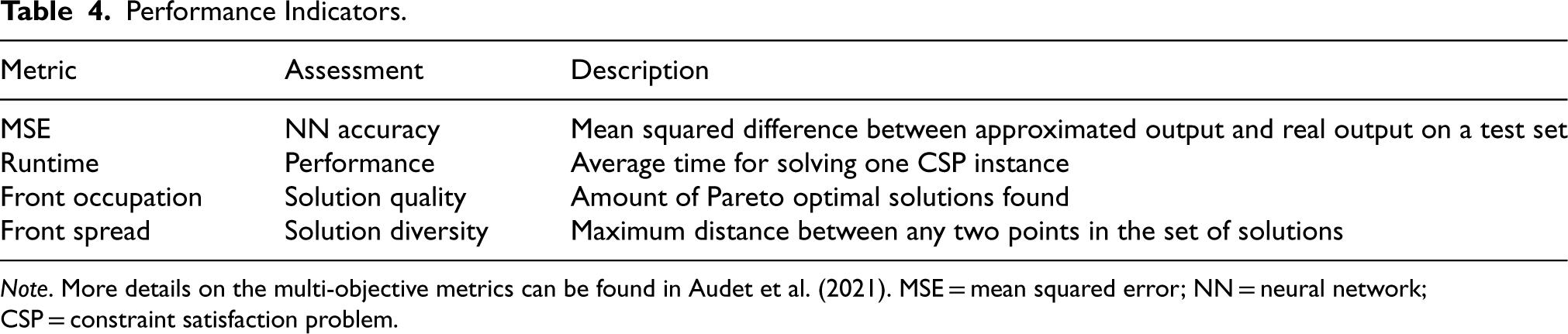
This section assesses the approach described in Section 3 by means of three experiments. Experiments 1 and 2 are based on a restaurant simulation. These show the effect of various design choices. Experiment 3 is based on the Food Wars simulation (Rasmussen and Wilensky, 2019), where we take a governing role over foragers with an aim to make them less hostile. The approach is assessed by various performance metrics, which are summarized in Table 4. These assess the runtime, accuracy, solution quality, and solution diversity.
Performance Indicators.
Performance Indicators.
Note. More details on the multi-objective metrics can be found in Audet et al. (2021). MSE = mean squared error; NN = neural network; CSP = constraint satisfaction problem.
Two further experiments, one based on a simulation model derived from a DEMO model and one based on a simulation study performed by other work, are reported in Andringa (2021). These two experiments highlight the generality of the approach by taking a problem description or enterprise model as input. Source code is available under MIT licence at https://www.doi.org/doi/10.4121/26776b70-225b-4091-ace3-e57324d0eaf1.
The Food Wars domain is more relevant to the focus of this article than the supply chain experiment from our preliminary work (Andringa and Yorke-Smith, 2021). Our previous work demonstrated the applicability and (initial) generalizability of the approach. Therefore, the supply chain experiment fitted well as its application is closely related to enterprise problems. However, this article puts more emphasis on performance and the utility of the approach. The supply chain experiment is less suitable for performance analysis as its underlying simulation environment is computationally exhaustive. Additionally, its output has large variance, since each initialization shuffles all connections in the supply chain network. This made generating sufficient simulation data an exhaustive approach. In contrast, the Food Wars domain allows for much better performance examination. Its corresponding simulator is much less computationally expensive, and its outputs have less variance. Furthermore, it is reasonable to classify the domain as being “complex,” due to its agent-based nature.
As stated, Experiments 1 and 2 use a restaurant simulation, introduced in Andringa and Yorke-Smith (2021). The restaurant buys ingredients periodically according to some buying strategy and processes them into various dishes. Its buying strategy is represented by an integer per resource that indicates the quantity being bought each period. Buying strategies have limitations, for example, due to seasonal ingredients. Resources can spoil if stored for too long. The restaurant has two objectives that characterize a tradeoff: it should not buy too many resources in order to minimize spoilage, but also should not buy too little in order to maximize the number of successful orders. The restaurant is interested in how its buying strategy affects its spoilage and success ratio.
The original problem has two objectives; extra objectives can be added by considering a spoil ratio per ingredient, and a success rate per dish.
Experiment 1: CSP Weight Sampling
The purpose of this experiment is to assess the performance of using low-discrepancy samplers to determine the weights for constructing the composite objective. As discussed in Section 3.3, our preliminary approach generated the weights uniformly at random. In this article, we adopt the use of Montgomery sampling to determine these. As shown in Table 5, low discrepancy sampling outperforms uniform sampling both in solution diversity (indicated by the higher front spread) and solution quality (indicated by the higher front occupation).
Experiment 1: Performance Indicators of Various Weight Sampling Methods.
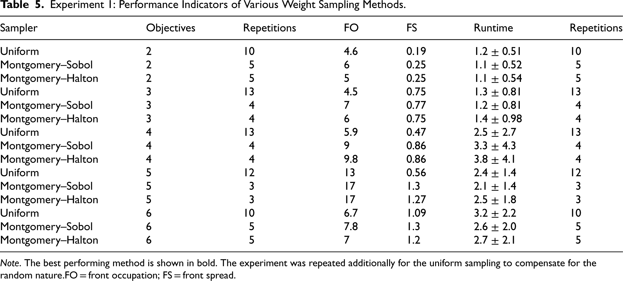
Experiment 1: Performance Indicators of Various Weight Sampling Methods.
Note. The best performing method is shown in bold. The experiment was repeated additionally for the uniform sampling to compensate for the random nature.FO = front occupation; FS = front spread.
As opposed to uniform sampling, Montgomery sampling is deterministic. The result is a more stable method to generate problems. This can be seen as an additional advantage of Montgomery sampling over the random approaches.
The purpose of this experiment is study the impact of the three activation functions discussed in Section 3.1.1. We experimented with two solvers, Gurobi Optimization, LLC (2022) and Kuchcinski and Szymanek (2013). The performance of Gurobi is expected to indicate the performance of a state-of-the-art solver, whereas JaCoP should provide insight into how architectural choice can impact performance. While JaCoP is not a commercial solver, unlike Gurobi, it does support modeling of the exponential quadratic term.
Table 6 provides the results. First, we notice Gurobi tends to outperform JaCoP. This shows the underlying solver has a large impact on the performance.
Experiment 2: Performance of Three Activation Functions.
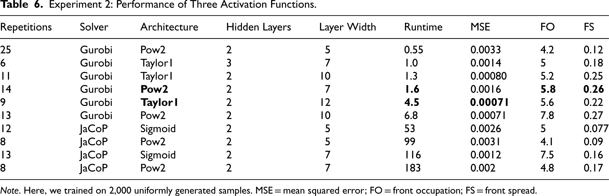
Experiment 2: Performance of Three Activation Functions.
Note. Here, we trained on 2,000 uniformly generated samples. MSE = mean squared error; FO = front occupation; FS = front spread.
Second, if we consider networks of the same network complexity, sigmoid tends to score best for reducing the mean squared error (MSE), followed by Power2, followed by Taylor1. However, this comes with a tradeoff. Sigmoid introduces an exponential quadratic term, which is not supported by the combination of Gurobi and MiniZinc, forcing the use of the slower JaCoP solver.
Third, Taylor1 is significantly faster than the other two, allowing us to use more complex networks. This shows the potential of using such output activation functions for NN embeddings in EML. The complexity of the network can be increased to an extent where it outperforms sigmoid in terms of accuracy, with no loss in runtime. However, there is a tradeoff. The proposed solutions are not as diverse as those found by the other activation functions. We suspect this to be a cause of a less robust network: Taylor1 scores better on average, but worse in worst-case scenarios.
Lastly, Table 6 shows that using deeper and wider networks improves accuracy, but comes with a tradeoff against increased runtime. The difference can be significant: going from layer width 7 to 10 increases the runtime.
The purpose of Experiment 3 is to assess the approach on a more complex problem domain. This experiment is based on the multi-agent based Fruit Wars NetLogo model (Rasmussen and Wilensky, 2019) and demonstrates how parameters in nonzero-sum economic environments impact cooperation and violence among agents. In this model, the agents collect fruit in order to survive. They do so by either wandering the map searching for fruit bushes or by attacking other agents to steal their fruit. Agents that survive pass on characteristics that influence their behavior to offspring. Input parameters, such as the bonus gained through collaborating or the maximum age foragers can achieve, are expected to have an impact on traits of the population.
Food Wars—Problem Description
Consider a governing position of some area of fruit foragers. The main objective is to let the foragers behave more peacefully. However, taking governing actions comes with a cost. As such, we are aiming for a proper tradeoff.
One can take action in two dimensions. First, one can choose to be accommodated in healthcare facilities, reflected by the max-age parameter. Second, one can give foragers who collaborate a bonus, reflected by the collaboration_bonus parameter. As an additional constraint, we want the average population, measured over a certain timespan, to be at least
The peacefulness of the population’s behavior is indicated by strength (how evolution resulted in a population with more strength), mortality-rate (how often foragers get killed), and proactive-aggression (how often foragers start to attack other foragers). A peaceful population has low values for all of them.
Additionally, it is essential that not all foragers die as a result of our policy. Therefore, we add an extra custom constraint, stating that the number of foragers should at least exceed 100 at the end of the simulation cycle.
Summarized, we are interested in minimizing both the input parameters, max-age and collaboration-bonus, and minimizing the output parameters strength, mortality-rate, and proactive-aggression, while maintaining a solid population.
Results
Table 7 shows results for this experiment. The solutions with a higher mortality rate are quite possibly a cause of lowering the max age. A lower max age would mean percentage-wise fewer people die of old age, thus the percentage of people that die because of other causes, such as being attacked, increases. The increased strength and proactive aggression are, however, less straightforward to explain. This can very possibly be due to noisy observations, as the simulation outputs tend not to show a consistent pattern.
Six Nondominating Solutions Found for the Food Wars Experiment.
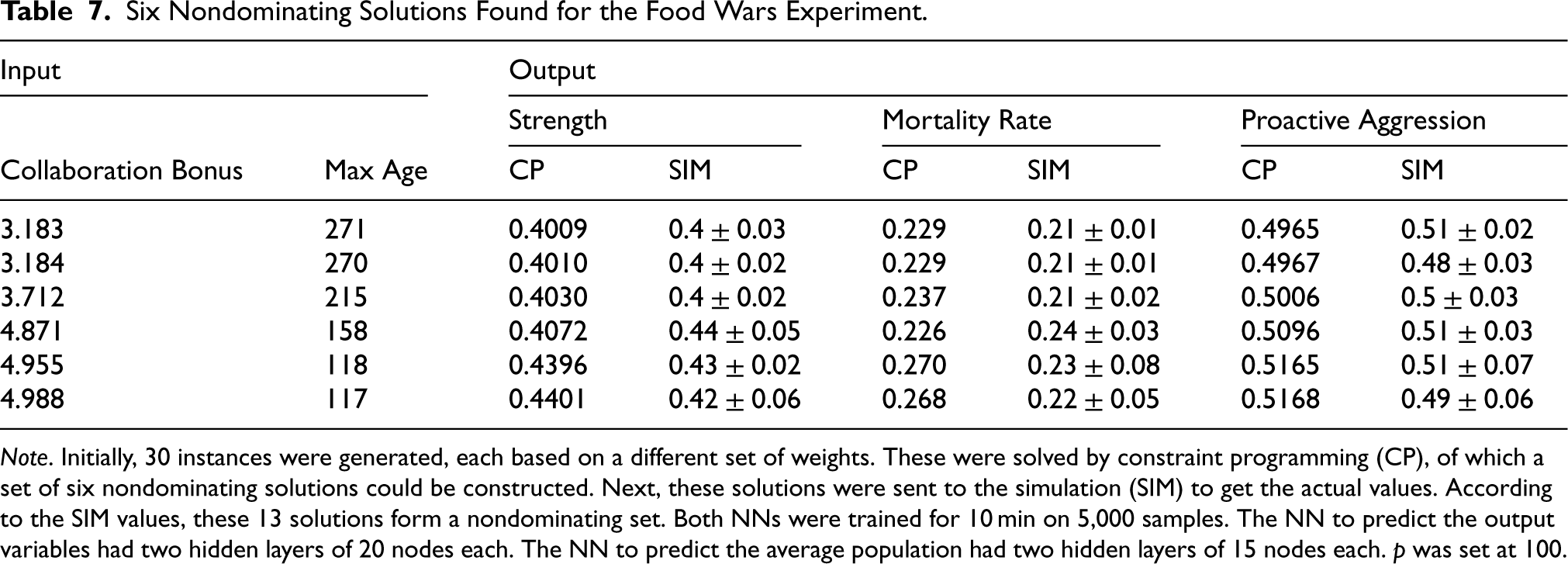
Six Nondominating Solutions Found for the Food Wars Experiment.
Note. Initially, 30 instances were generated, each based on a different set of weights. These were solved by constraint programming (CP), of which a set of six nondominating solutions could be constructed. Next, these solutions were sent to the simulation (SIM) to get the actual values. According to the SIM values, these 13 solutions form a nondominating set. Both NNs were trained for 10 min on 5,000 samples. The NN to predict the output variables had two hidden layers of 20 nodes each. The NN to predict the average population had two hidden layers of 15 nodes each.
Although the outputs tend not to differ drastically, the inputs do. This might indicate that the optimal solutions have a similar state, but that they can be achieved in several ways. Differently stated, increasing the collaboration bonus has a similar effect as increasing max age and vice-versa. This should help assist the DM to make a proper decision, where it can take into account how costly it thinks increasing the input parameters would be.
Furthermore, trivial examples where the inputs are minimized toward extreme values are not included. This is an effect of the additional constraint regarding the lower bound for the population. According to our CP model, feeding inputs that strictly dominate the found solutions (i.e., inputs where both max-age and collaboration bonus are lower with respect to at least one of the found solutions), will result in killing too many foragers.
The experiments reported have offered various insights which can be summarized as follows: Using low-discrepancy sampling, in our approach through Montgomery sampling, to generate a set of problem instances results in more qualitative and diverse Pareto approximations. Deeper and wider networks tend to provide more accuracy at a cost of increased runtime. Discarding quadratic terms from output activation functions significantly decreased runtime. Our experiments show that this was paired with a cost of decreased solution diversity. The approach can be applied to a diverse range of applications due to its automatic procedure and flexibility in modeling the problem.
For enterprise SO, this article addressed the crucial question of how to find optimal simulation inputs more effectively. The proposed approach adopts a meta-model in the form of an NN to capture simulation behavior, and embeds the NN automatically into a soft CP model.
We demonstrated the performance sensitivity of the approach by experiments on three problems. In contrast to our previous work, we directly optimize toward a weighted objective instead of the possibilistic approach. We argued in Section 3.3 why this better fits the approach.
The experiments demonstrated how Montgomery sampling reduces the number of simulation calls necessary to obtain the same amount of insight in a stable and deterministic manner. Although for this application the results have shown to be effective, the discrepancy properties—which Sobol and Halton sequences have—are not kept intact. It can be interesting to experiment with an alternative sequence that maintains these properties while adhering to the summation constraint. This is left as future work; we provide a description of an algorithm that could potentially work in Appendix A.
In a highly complex real-world scenario, the number of parameters and observables can be much bigger compared to the experiments performed for this article. A major impact on performance is the solution space—number of input variables and objectives—of the CSP. If the DM is encountering performance issues, we would advise the DM, instead of creating a “master CSP” that addresses all various problems at once, to focus on a subset of input variables and objectives. A good strategy here might be splitting up the CSP and solving the shared CSPs independently.
Furthermore, in this article, we showed activation function Taylor1 performs remarkably well compared to Power2 and Sigmoid in terms of reducing the MSE of the trained network. This shows the potential of using linear-oriented activation functions, when the NN is to be embedded in a CSP. However, these activation functions underperformed in terms of solution diversity. We suspect this to be the cause of network robustness. This issue might be overcome by using a different NN architecture or training strategy. We should note that we only considered a single alternative to an output activation function without a quadratic term. As mentioned in Section 3.1.1, the sigmoid was the only activation function among those experimented with that has a different input for each output and vice versa. It can be interesting to experiment with other activation functions that also have this property and evaluate whether these are more robust. This is left as future work for the EML community.
Building on the approach of this article, it can be interesting to consider constraint acquisition (Bessiere et al., 2017). Here, the CP model is allowed to make simulation calls to obtain more knowledge when it considers it possesses too little. This gives up a form of flexibility, in that solving becomes dependent on the simulation runtime. However, it is expected to be more accurate than our approach as it can consult the simulation model in case of doubt. Constraint acquisition is different from black box optimization, and allows exploitation of the model structure (see Table 2). An interesting follow-up study would be a performance comparison between the proposed methodology, constraint acquisition, and other multi-criteria optimization methods such as evolutionary search.
Footnotes
Acknowledgments
Thanks to the anonymous reviewers. The authors thank Aaron M. Montgomery for his help designing the weight sampling method and Marco Loog for his input on activation functions.
Funding
The authors disclosed receipt of the following financial support for the research, authorship, and/or publication of this article: This research was partially supported by TAILOR, a project funded by the EU Horizon 2020 research and innovation programme under grant number 952215.
Declaration of Conflicting Interests
The authors declared no potential conflicts of interest with respect to the research, authorship, and/or publication of this article.

Notes
Appendix A Improved Montgomery Sampling Algorithm 2
Appendix B NN Embedding in MiniZinc,Supply Chain Experiment