Improving Your DOE - Analysis with Response Transformations

Abstract

The typical data analysis from a designed experiment (DOE) uses analysis of variance (ANOVA). Characteristics of a good model include having statistically significant model terms (and doing model reduction to remove insignificant terms), along with good lack of fit statistics and ideally, higher adjusted R-squared and predicted R-squared values. Beyond this, it is important that the underlying statistical assumptions for the use of ANOVA are verified. These assumptions include:

• The residuals (difference between actual and predicted values) are independent

• The residuals are normally distributed

• They have a constant variance across the predicted response range.

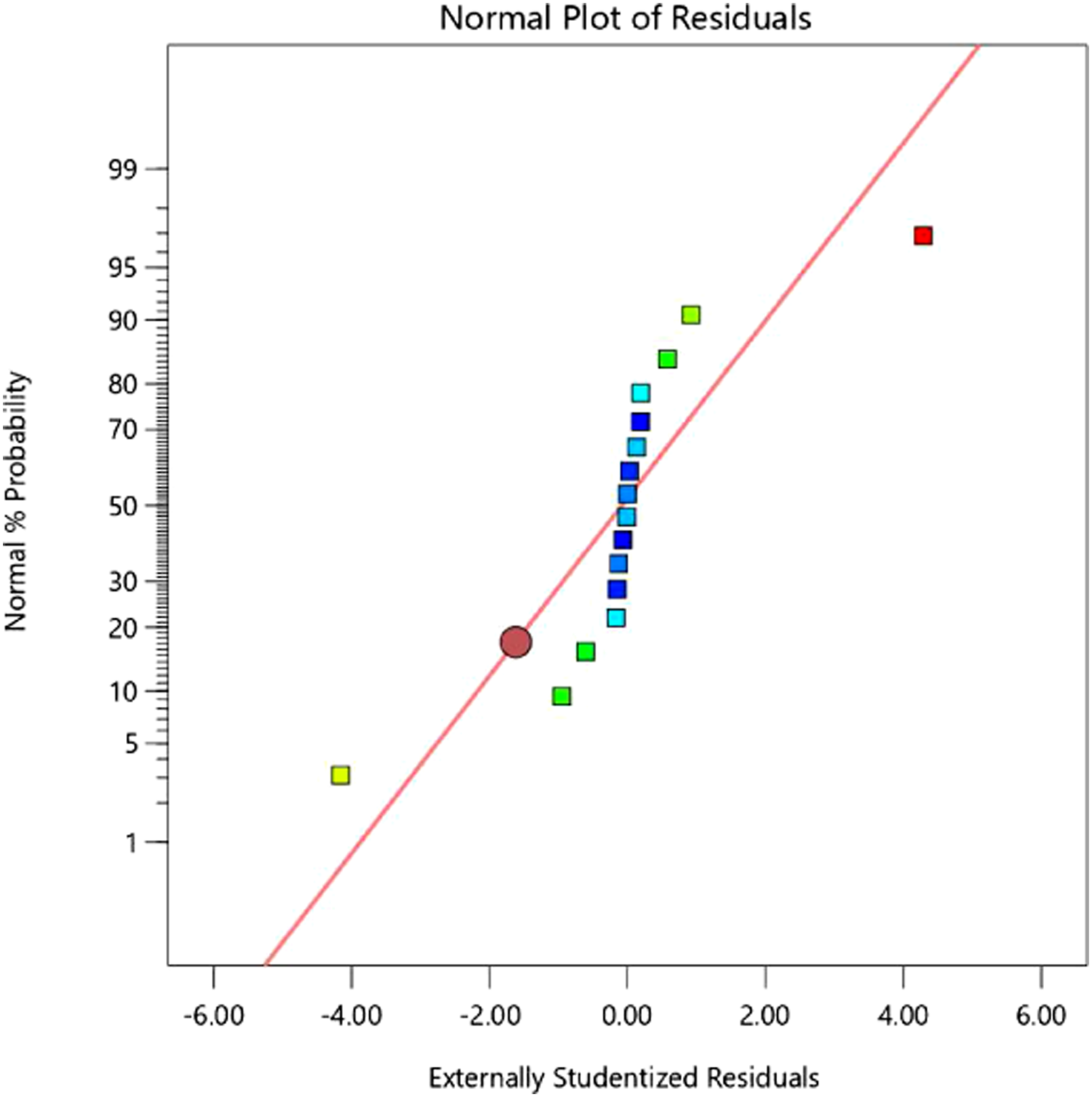
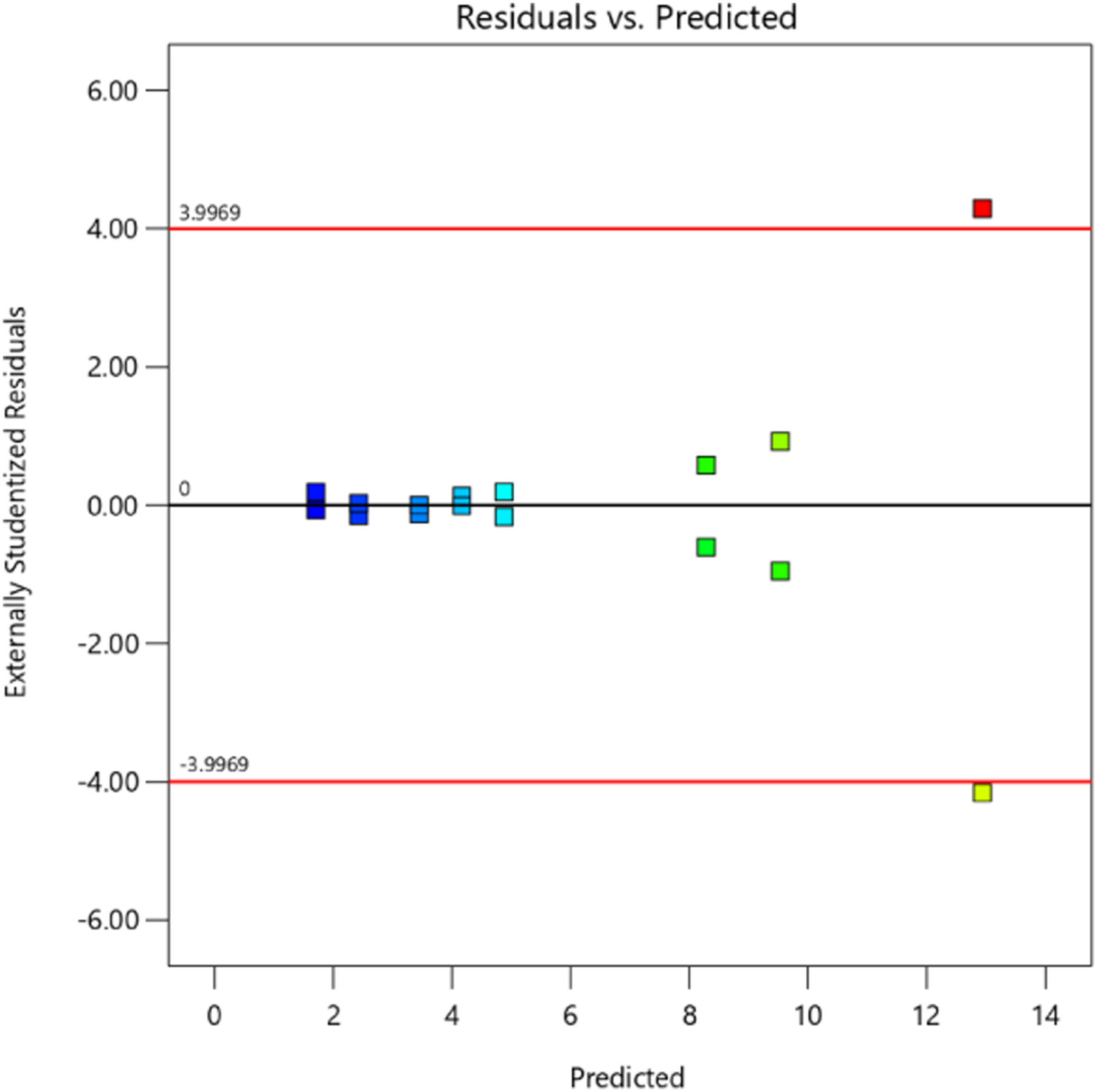
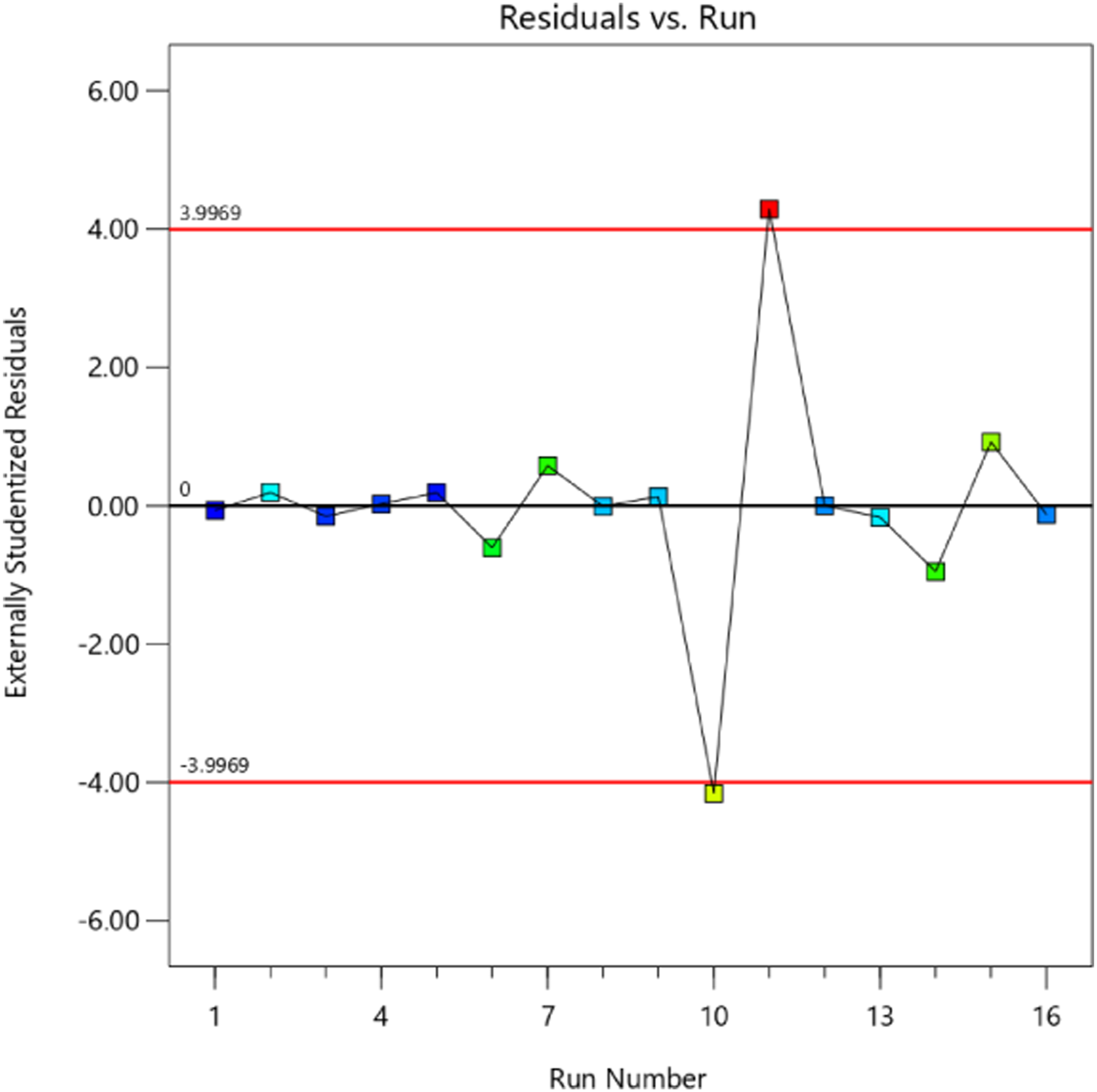
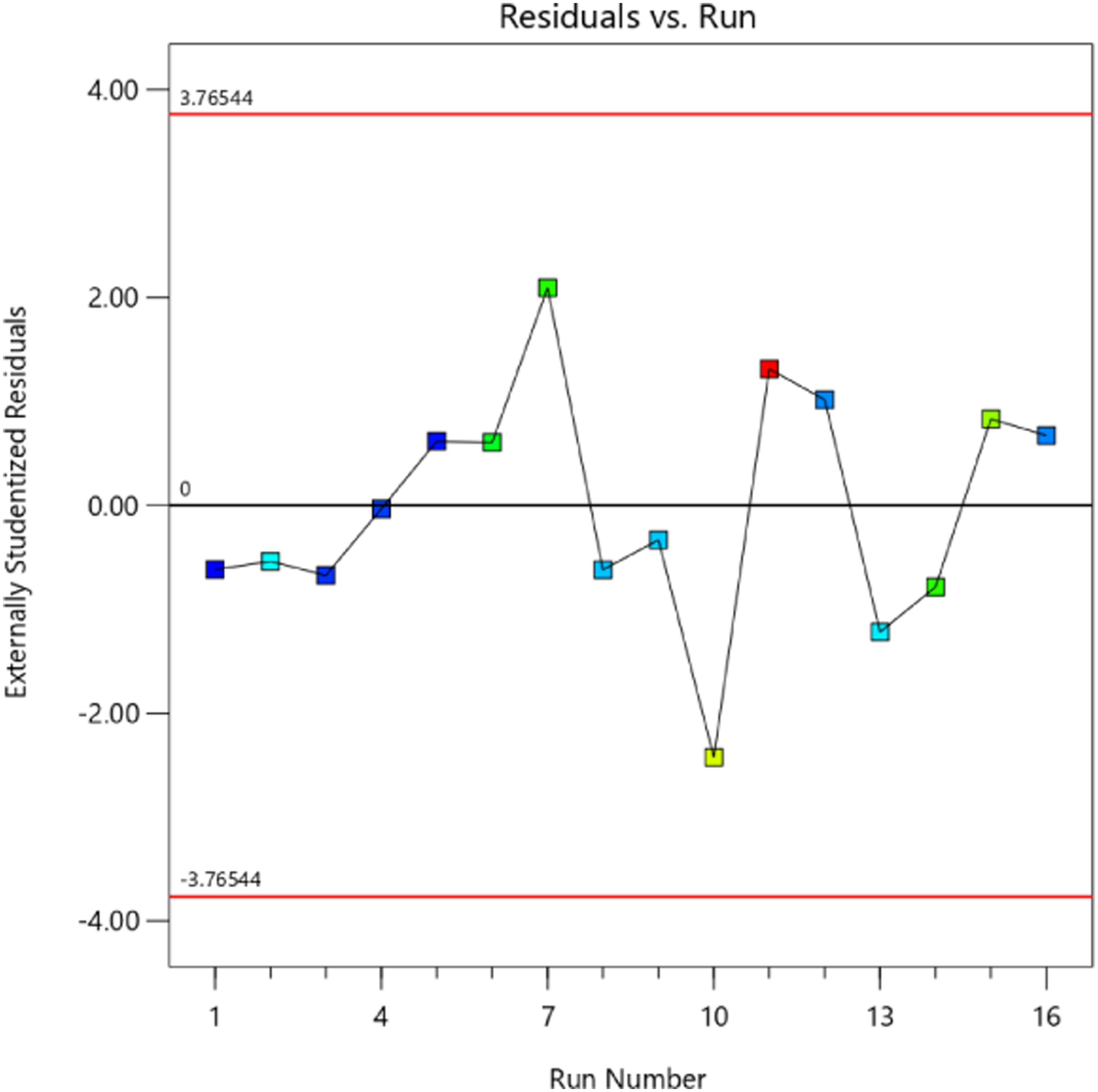
Design-Expert® software provides extensive diagnostic capabilities to check if the statistical assumptions underlying the data analysis are met. Residual diagnostic graphs are used to visually confirm these assumptions. These assumptions are violated in Figures 1 to 3:

• Normal Plot of Residuals should be a straight line to confirm normality. Watch for a strong S-shaped curve.

• Residuals versus Predicted plot should be a random scatter, with a similar vertical spread of the residual points from left to right, to confirm constant variance. Watch for a “megaphone” or “horn” shape that shows increasing variation with larger predicted values.

• Residuals versus Run plot should be random, with no time-ordered trends or outliers (points outside the red lines).

Figure 1.

Normal plot of residuals.

Figure 2.

Residuals versus predicted.

Figure 3.

Residuals versus run.

When these residual plots show substantial violations of the assumptions, it is time to consider a response data transformation. A data transformation means that the response values are rescaled - for example, put on a log or square root scale. Then the data is re-fit to a model and all assumptions are checked again. Power-law transformations mean that each data point is “raised to the power of” a value designated by lambda (λ). Some typical power-law transformations and examples for their use are:

• Square Root (λ = 0.5) – count, frequency data

• Base 10 or Natural log (λ = 0) – variance or growth data

• Inverse (λ = −1) – rate or time-based data

The appropriate choice of a response transformation relies on both subject-matter knowledge and/or statistical considerations. Choosing the best power transformation is much easier with the Box-Cox plot (Figure 4). Based on the fitted model, the residual sum of squares (error) is plotted against the various power transformations (lambda −3 to + 3). The best transformation is found wherever the residual SS is smallest (the curve is at a minimum). In addition to the calculated “best” transformation, a 95% confidence interval surrounds this value (red lines), so that the experimenter can confidently choose any transformation within that statistical interval. In Figure 4, the confidence interval includes the log transformation, so that is applied to the data.

Figure 4.

Box-cox plot – no transform.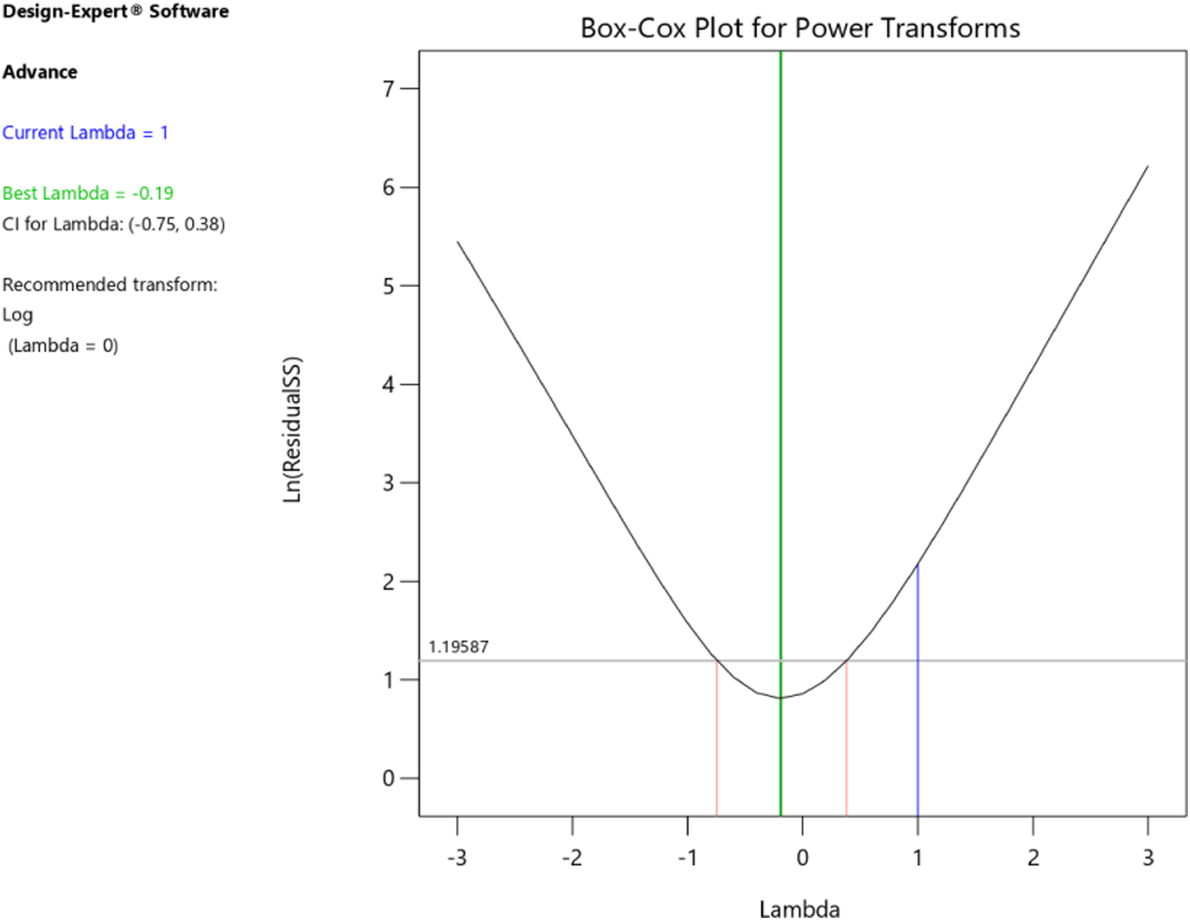

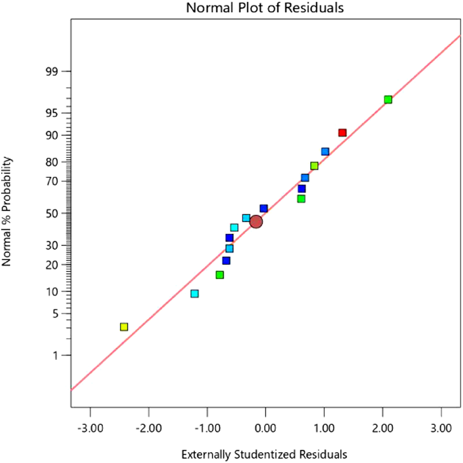
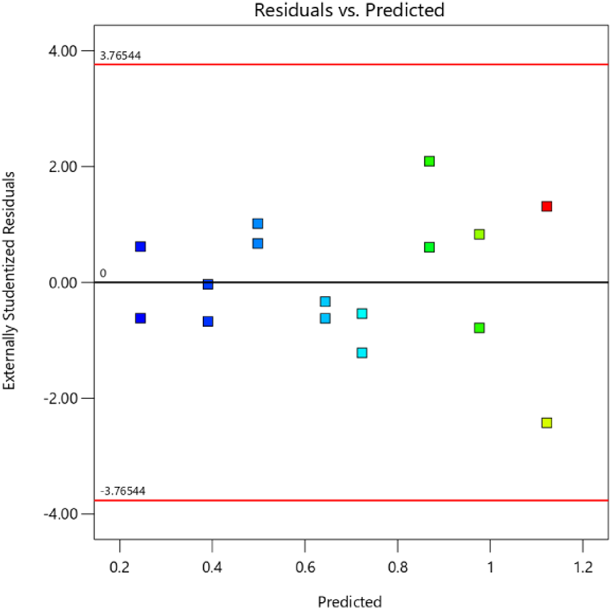
After the response data has been transformed (put onto the appropriate scale), the data is re-fit to an updated model and the ANOVA and residual diagnostics are checked again. The new Box-Cox plot (Figure 5) confirms that log is still best. The ANOVA assumptions are now satisfied, as shown in Figures 6 to 8.

Figure 5.

Box-cox plot – log transform.

Figure 6.

Normal plot of residuals- after log transform.

Figure 7.

Residuals versus predicted- after log transform.

Figure 8.

Residuals versus run- after log transform.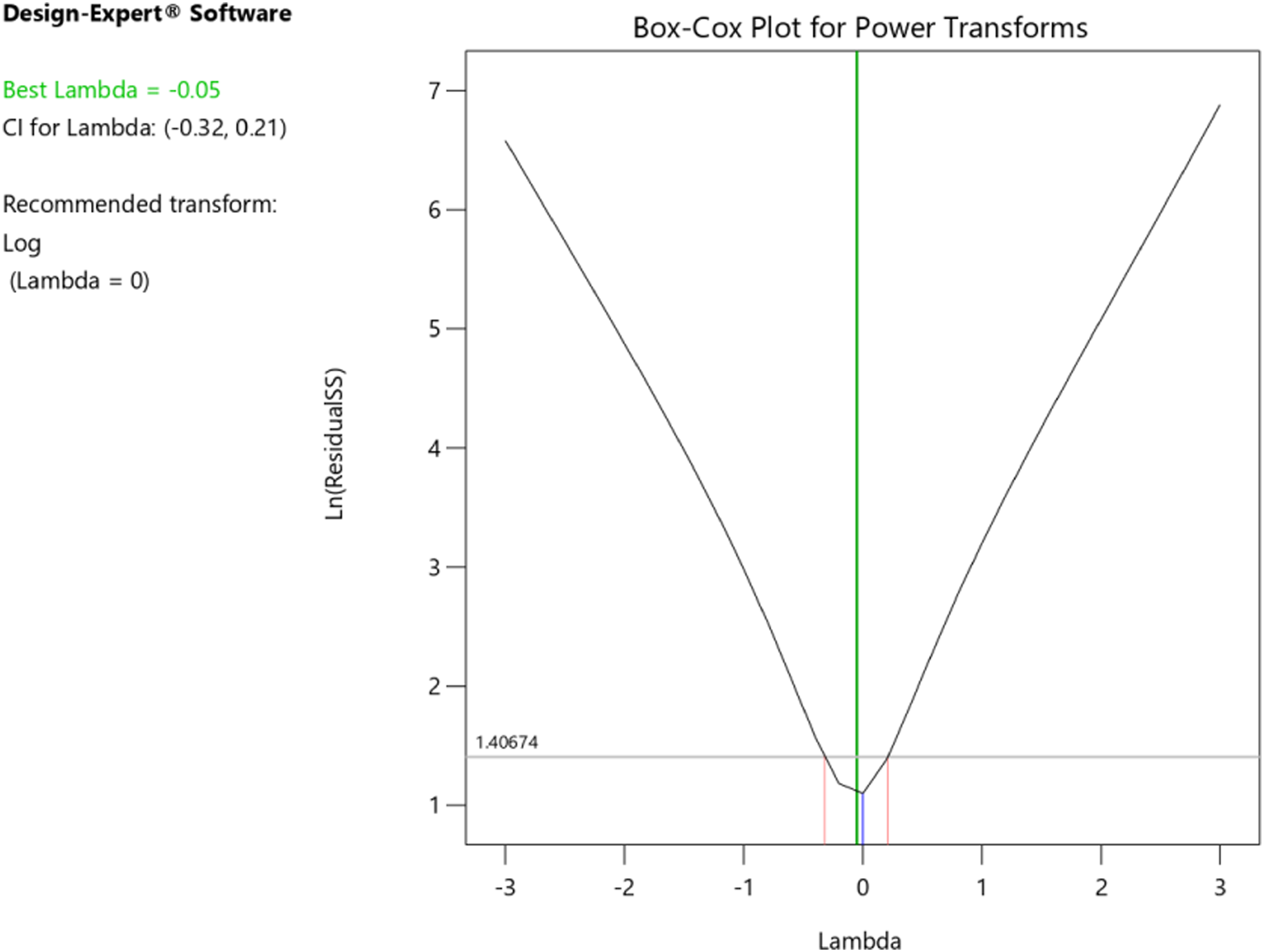

In summary, when you first fit a model, check the ANOVA residual diagnostics. If there are any strange patterns, consider a response transformation. Use the Box-Cox plot as a guide to determine the best option, taking into account subject matter knowledge. Confirm the diagnostics after re-fitting the model.

Good luck with your DOE data analysis!

Footnotes

Biography

Shari Kraber has a BS in Industrial Engineering, Iowa State University and MS in Applied Statistics, Rochester Institute of Technology and is a registered PE in Minnesota. She is a consultant with Stat-Ease, with over 25 years of experience teaching engineers and technical professionals how to design and implement design of experiments. Shari draws on her process engineering experiences at 3M and Frigidaire where she implemented statistical quality tools such as statistical process control and DOE. As the Stat-Ease Workshop Manager, she now devotes her considerable energy, experience, and leadership skills to workshops on DOE, teaching others how to make breakthroughs.