Neural networks for critical high temperature component life prediction

Abstract

The aim of the present research was to subject a well known parametric model and a neural network model to an acid test of extrapolation in order to determine which can produce improved long term creep rupture life predictions for 2·25Cr–1Mo steels. Linear, squared and cubic parametric models were used and the accuracy of the predictions assessed by calculating the mean percentage absolute error. Many different neural network geometries were developed and the accuracy of the predictions was assessed again by calculating the mean percentage absolute error. As the predictions are concerned with the long term rupture life of components, the accuracy below 60 MPa is of the greatest importance. A neural network model with a 2–5–5–1 architecture provided the lowest error for predictions below 60 MPa, compared to other neural networks and the parametric models, and is therefore the optimum model from this study for predictions of long term rupture creep life for a 2·25Cr–1Mo steel.

Keywords

Neural networks Creep Life prediction Parametric model Steel

Introduction

Creep

Creep is defined as the time dependent and permanent deformation of materials when subjected to a constant load or stress. Creep is considered a limiting factor in the lifetime of a component. Normally, creep only becomes important in metals above temperatures of 0·3–0·4 times the absolute melting temperature (0·3–0·4T_m).¹

2·25Cr–1Mo steel is an established ‘creep resistant’ alloy, used extensively in high-temperature boiler pressure parts.² This good creep rupture behaviour can be explained by the interaction between molybdenum and carbon in the steel. When steel contains substitutional (Mo) and interstitial (C) elements in solution, they can interact to form atom pairs or clusters. These clusters can form dislocation atmospheres that obstruct dislocation motion, imparting additional strength to the steel. This process is termed interaction solid solution hardening.³

When performing life assessment of high temperature components against creep rupture, short term data are used to predict the long term rupture life. To perform the tens of thousands of experimental hours required until rupture at lower stresses would take far too long and is impractical. Methods of predicting the long term rupture life of components are therefore used. The 4-theta concept⁴ and 6-theta concept⁵ utilise information from the whole creep curve when available. The Monkman–Grant equations^6,7 and Manson and Haferd⁸ model are examples of parametric models, and more recent parametric techniques are the minimum commitment⁹ and the Soviet methods,¹⁰ which are essentially combinations of the ‘older’ parametric methods. Two methods of prediction were investigated in this study: the Larson–Miller parametric model, and an artificial neural network model. The Larson–Miller method was proposed¹¹ and has been investigated previously with respect to this specific steel.^12,13 Neural network models have previously been used with respect to life predictions in fatigue of aircraft components,¹⁴ elevated temperature creep–fatigue interactions¹⁵ and fatigue of composites.¹⁶

Parametric model

The parametric model is based on the Larson–Miller model. This is an extrapolation technique for determining the long term rupture life from short term experimental data. The Larson–Miller theory is based on the assumption that creep is a rate process and therefore complies with the Arrhenius equation. This extrapolation depends upon the relationship between stress σ, temperature T and rupture time t_r. The Arrhenius equation is manipulated to obtain the Larson–Miller parameter¹⁷ 1 where P_LM(σ) is the Larson–Miller parameter as a function of stress and C is a constant.

Neural networks

Neural networks are termed neural networks because they are a network of interconnected elements. They are inspired by the way the densely interconnected, parallel structure of the biological brain, processes information.¹⁸ The components used in a neural network are designed to behave like biological neurons,¹⁹ although biological neurons are far more complex than these artificial models. Essentially, neural networks are statistical models of real world systems, built by tuning a set of parameters.

The net topology chosen for this application was the Multi–Layer perceptron. This example is a feedforward network. It is termed a feedforward network because the outputs of units in one layer are only connected to the inputs of units in the next layer, i.e. the information is always flowing from the inputs to the outputs.²⁰ Perceptrons can be used for classification or as non-linear estimators, the latter being used in this project, with an example of a multilayer perceptron shown in Fig. 1.

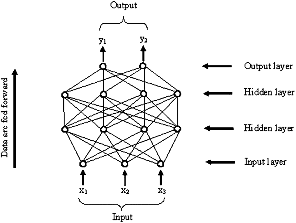
Example 3–4–4–2 multilayer perceptron including input, hidden and output layers

The notation used in Fig. 1 (3–4–4–2) is a simple way of expressing the number of nodes in each layer, starting with the input layer, through to the output layer.

The first layer is termed the input layer. The inputs are connected to the outside world. This is usually a ‘fan-out layer’, and means that a unit in this layer has one input and several outputs each with a value equal to the input. Therefore, no processing takes place in this layer.²⁰

The next layer is termed the hidden layer because neither the inputs nor the outputs can be seen from the outside. This is the first layer in which processing takes place. The example in Fig. 1 displays two hidden layers but there can be many hidden layers.

The final layer is termed the output layer. The outputs are connected to the outside world. It has several inputs from the units in the previous hidden layer, and its outputs are the outputs of the network.

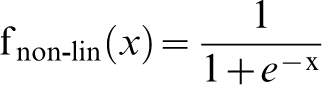
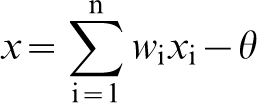
This type of network is called a ‘fully connected multilayer network’. This means that every output from every node in one layer is connected to every input of every node in the next layer.²¹ The role of a node is to sum its inputs, subtract a bias or threshold term θ and pass the result through a non-linear function known as the activation function; in this case, it is the sigmoid function²² 2 where 3 where n is the number of inputs, w_i is the input weighting, x_i is the input value and θ is the bias or threshold term.

The output is then transferred to each of its output connections. The interconnections have an input and output end, and also perform a simple arithmetic function. Every interconnection has a weighting w_i related to it, i.e. for an input x_i, its output is w_ix_i.

Training of the network is concerned with finding the optimum weighting values and bias terms in order to produce accurate output predictions. Training of a neural network involves passing a set of examples of input–output pairs through the network. Input values are applied to the input layer and the output that is generated is compared with the correct output, the difference being the error. The sum of the squares of the errors is minimised by tuning the weights and bias terms; this can take many passes through the training data, and is known as supervised learning. The network is said to have converged when the total squared error has become acceptably low; therefore, these weights and bias terms are retained. The training is stopped before overfitting (the program does not generalise well to new data) occurs. The network is then able to produce accurate output values for input values that were not included in the training data. This is termed generalisation.²³

Predictive modelling methodologies

The source data are taken from the MAF batch of the National Research Institute for Metals Creep Data Sheet No. 3B²⁴ (data sheets on the elevated temperature properties of 2·25Cr–1Mo steel for boiler and heat exchanger seamless tubes). The boiler tubes used in the programme were sampled at random from commercial stocks produced in Japan using an electrical arc furnace. Each tube had an outside diameter of 50·8 mm, a wall thickness of 8 mm and a length of 5000 mm.

Creep tests were conducted on cylindrical specimens with a gauge length of 30 mm at constant load with a loading accuracy of 0·5. Temperatures between 373 and 873 K were controlled to 3 K and temperatures in excess of 873–4 K. A number of different heat treated specimens were tested. The MAF batch of specimens were obtained from rotary pierced and cold drawn ingots and heat treated for 1200 s at 1200 K followed by 7800 s at 993 K and air quenched. The material had a grain size of 6 (ASTM) and a Rockwell hardness of 78 HRB. The test temperatures varied from 723 to 923 K and the stress varied from 14 to 333 MPa. Over these ranges, some 60 specimens were tested, and information on time to failure, elongation, reduction of area and the minimum creep rate were collected.

Parametric model

The first prediction method utilised a parametric model (Larson–Miller model). The equation used is presented below 4 where t_f is the time to rupture (h), d₁, d₂, d₃, d₄ and d₅ are constants, σ is the stress (MPa) and T is the temperature (K).

The first model utilised only the linear stress term (i.e. d₃ and d₄ were set to zero). ln (t_f) values were then calculated for the various stresses and temperatures using constants determined by a parameter optimisation routine. The aim was to minimise the squared error between the actual ln (t_f) and the predicted ln (t_f) by altering the values of the constants. A graph comparing the actual data to the predicted data could then be produced for this linear model. This process was then repeated for the squared model, utilising the linear and squared stress terms in equation (4) (i.e. only d₄ was set to zero), and the cubic model, utilising the linear, squared and cubic stress terms in equation (4) (i.e. no constants set to zero).

The comparable values drawn from these models are the mean percentage absolute error values for stresses below 60 MPa and stresses above 60 MPa (60 MPa is the creep mechanism threshold observed by Yamauchi.²⁵ The distinction is made between these two sets of data because there is a distinct difference between the gradients of the curves on the ln (tf) v. stress graph above and below the threshold, which is the nature of the problem when making long term (lower stress) rupture life predictions. This provided values for easy comparison between the linear, squared and cubic models in order to determine which provided the most accurate predictions of the long term rupture life, but also what effect improving the accuracy of predictions at lower stress would have on the predictions at higher stress.

Neural network model

The second modelling technique required the formulation of a suitable neural network. The type of network chosen was a multilayer perceptron consisting of four or three layers, two inputs, no more than five nodes in each of the hidden layers, and one output. An autodesigner function was also utilised and was set constraints of a maximum of four layers but unlimited nodes in the hidden layers.

The source data consisted of 47 different stress–temperature–time sets. Stress (MPa) and temperature (K) were set as the inputs and ln (time to rupture, t_f) (h) was set as the output. All the data point to the right of the 60 MPa creep mechanism threshold observed by Yamauchi were allocated as the training data; five of these points were set randomly as verification data (∼10 of the total number of datasets). The purpose of the verification data was to verify the predicted results obtained when using weights from the training data. The remaining 11 points to the left of the 60 MPa creep mechanism threshold were then set as test data.

The first network architecture was set to 2–5–5–1, then 2–5–4–1 for the second generated network, then 2–5–3–1 for the third, down to a size of 2–1–1. Once each network was created, the multilayer perceptron was then trained.

The ‘conjugate gradient descent’ method was used as the training method for each network generated. Conjugate gradient descent is a batch update algorithm; it calculates the average gradient of the error surface for all cases, before updating the weights once at the end of the epoch. On each epoch, the entire training set is fed through the network, and used to adjust the network weights and bias terms. Conjugate gradient descent works by conducting a succession of line searches across the error surface. It first calculates the direction of steepest descent and projects a straight line in that direction, and then locates a minimum along this line. Consequently, further line searches are conducted (one per epoch). Once a point close to a minimum is found, the minimum can be located very rapidly. Training stops and the weights are retained when the training data and verification data errors cannot be reduced any further.

The network was run to obtain predicted outputs for input values, using the weights determined via training. The resulting outputs are the ln (t_f) as predicted by the network, the actual or target ln (t_f) from the source data and the difference between them (i.e. the error) for each stress–temperature set. Once each network was designed, run and the results taken, the autodesigner was used with the properties stated earlier to obtain a network and results to compare with those created previously.

In order to obtain comparable values from the data, the squared error was calculated from the error between the predicted and target output. The average squared error and sum of the squared errors were calculated for the training, verification and test datasets. The percentage absolute error was calculated for the test data (i.e. the data points to the left of the 60 MPa creep mechanism threshold) and also the points above 60 MPa, and the mean percentage absolute error. This gave a single value for assessing the accuracy of each network in predicting the long term (lower stress) rupture life.

Model comparison

The values of the mean percentage absolute error obtained from both models for the long term (lower stress) rupture life predictions, i.e. to the left of the 60 MPa creep mechanism threshold, were then compared in order to determine which modelling method was the most accurate in predicting the long-term rupture life for a 2·25Cr–1Mo steel. The values above 60 MPa were also compared to determine the higher stress accuracy.

Results

Parametric prediction

The objective of performing the parametric model was to compare the accuracy of the predictions for the ln (time to rupture, h) above 60 MPa and below 60 MPa for the linear, squared and cubic parametric models, and to also obtain values to compare with the subsequent neural network models.

The predicted ln (time to rupture, h) values were attained for each of the parametric models and plotted versus stress (MPa). These were compared to the experimental data to assess the accuracy between the models.

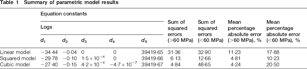
It is not clear which parametric model is most accurate at predicting the long term rupture life from the three graphs alone (Figure 2–4); therefore, the mean percentage absolute error was calculated for the predicted data compared to the actual data for the low stress group (below 60 MPa) and the high stress group (above 60 MPa). Table 1 shows that the cubic model (4·24) had a smaller error than the squared model (4·81) for the stress group above 60 MPa, whereas the linear model (11·23) had the greatest error. For the stress group below 60 MPa, the squared model (10·23) has by far the lowest error, the second is the linear model (17·88), and finally the cubic model (20·50) has the greatest error. The percentage error of each model at varying stresses is illustrated in Fig. 5. From the graph in Fig. 5, the percentage error extremes of the parametric models can be seen for the stress group below 60 MPa, this range being 2·91–30·90.

ln (time to rupture) v. stress for 2·25Cr–1Mo steel with outputs predicted by linear model compared to actual measured data

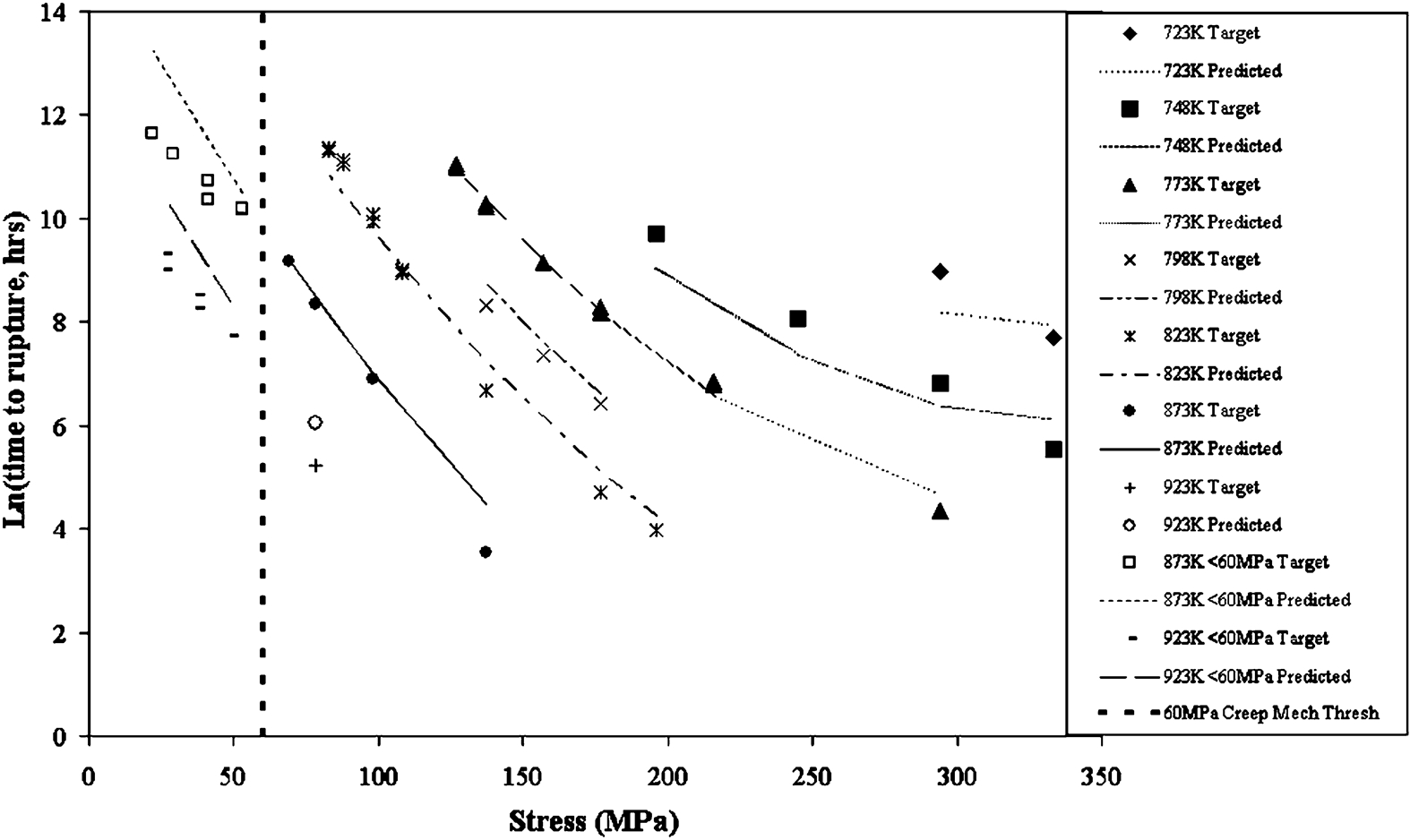
ln (time to rupture) v. stress for 2·25Cr–1Mo steel with outputs predicted by squared model compared to actual measured data

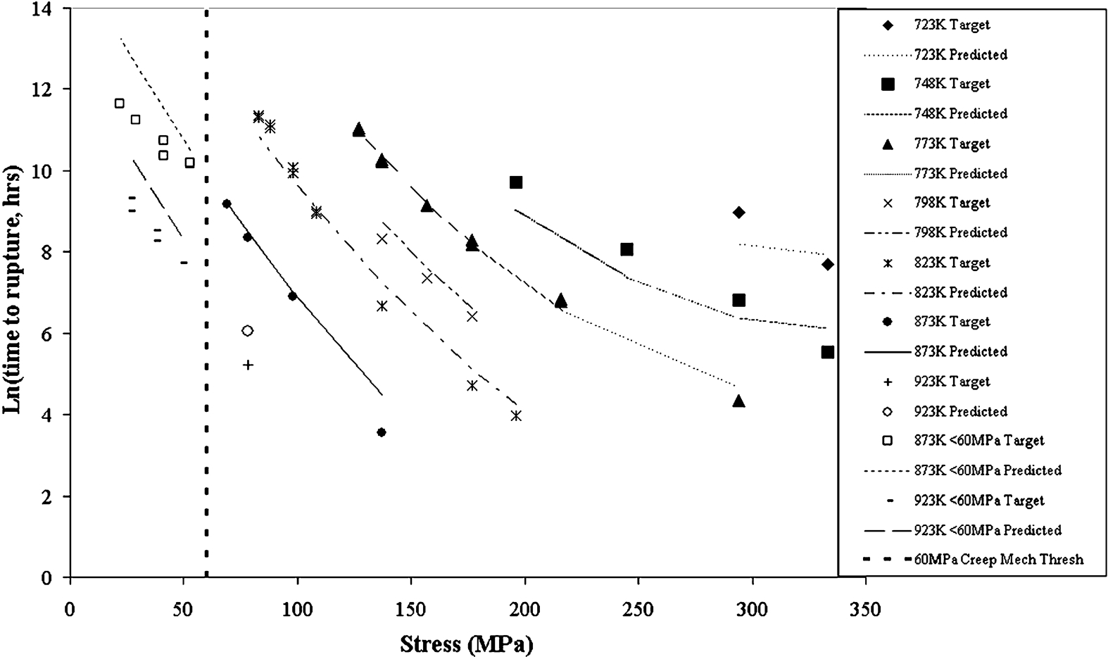
ln (time to rupture) v. stress for 2·25Cr–1Mo steel with outputs predicted by cubic model compared to actual measured data

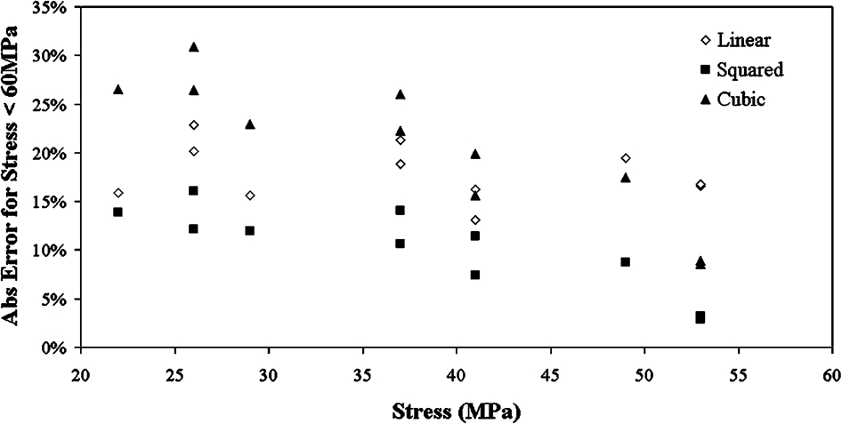
Absolute error () v. stress (<60 MPa) for parametric models

Table 1

Summary of parametric model results

	Equation constants					Sum of squared errors (>60 MPa)	Sum of squared errors (<60 MPa)	Mean percentage absolute error (>60 MPa),	Mean percentage absolute error(<60 MPa),
	Logs
	d ₁	d ₂	d ₃	d ₄	d ₅
Linear model	−34·44	−0·04	0	0	39419·65	31·36	32·90	11·23	17·88
Squared model	−29·78	−0·10	1·5×10⁻⁴	0	39419·66	6·13	12·66	4·81	10·23
Cubic model	−27·40	−0·15	4·2×10⁻⁴	−4·7×10⁻⁷	39419·67	4·84	48·65	4·24	20·50

Neural network prediction

The objective of formulating the neural networks was to compare the accuracy of the ln (time to rupture, h) predictions obtained for different network geometries and compare these with the results taken from the parametric models. The predicted ln (time to rupture, h) values were produced for each of the neural networks and the mean percentage absolute error calculated for stresses below 60 MPa. Table 2 gives a summary of the values obtained from each neural network design.

Table 2

Designed neural network summary

	Mean percentage absolute error (>60 MPa),	Mean percentage absolute error (<60 MPa),	Training average squared error	Verification average squared error	Test average squared error	Training sum of the squared errors	Verification sum of the squared errors	Test sum of the squared errors
2–4–7–1	8·02	2·90	0·517	0·007	0·113	16·020	0·036	1·242
2–5–5–1	3·98	2·35	0·114	0·352	0·076	3·527	1·758	0·832
2–5–4–1	3·86	12·07	0·097	0·269	1·662	2·998	1·345	18·285
2–5–3–1	4·28	7·18	0·107	0·230	0·616	3·327	1·151	6·773
2–5–2–1	5·03	13·19	0·135	0·937	2·158	4·188	4·683	23·743
2–5–1–1	3·74	9·65	0·129	0·158	1·062	4·000	0·790	11·682
2–4–4–1	3·77	6·43	0·095	0·242	0·460	2·934	1·211	5·060
2–4–3–1	3·93	14·05	0·105	0·303	2·241	3·241	1·514	24·648
2–4–2–1	4·12	11·46	0·091	0·554	1·556	2·822	2·771	17·121
2–4–1–1	4·27	10·83	0·110	0·327	1·373	3·419	1·634	15·107
2–3–3–1	3·96	9·21	0·097	0·282	0·991	2·997	1·409	10·901
2–3–2–1	4·07	11·41	0·105	0·386	1·476	3·249	1·932	16·236
2–3–1–1	4·13	4·85	0·102	0·356	0·249	3·163	1·779	2·744
2–2–2–1	4·67	4·68	0·194	0·172	0·252	6·024	0·862	2·770
2–2–1–1	4·47	9·29	0·120	0·298	1·006	3·722	1·489	11·062
2–1–1–1	12·46	12·26	1·237	0·465	1·731	38·339	2·323	19·038
2–5–1	3·76	8·96	0·101	0·187	0·939	3·137	0·936	10·328
2–4–1	3·84	5·05	0·102	0·178	0·297	3·163	0·889	3·263
2–3–1	3·63	10·80	0·078	0·347	1·335	2·432	1·733	14·687
2–2–1	3·77	8·04	0·085	0·339	0·738	2·625	1·693	8·120
2–1–1	12·46	28·73	1·126	0·978	7·682	34·915	4·892	84·503

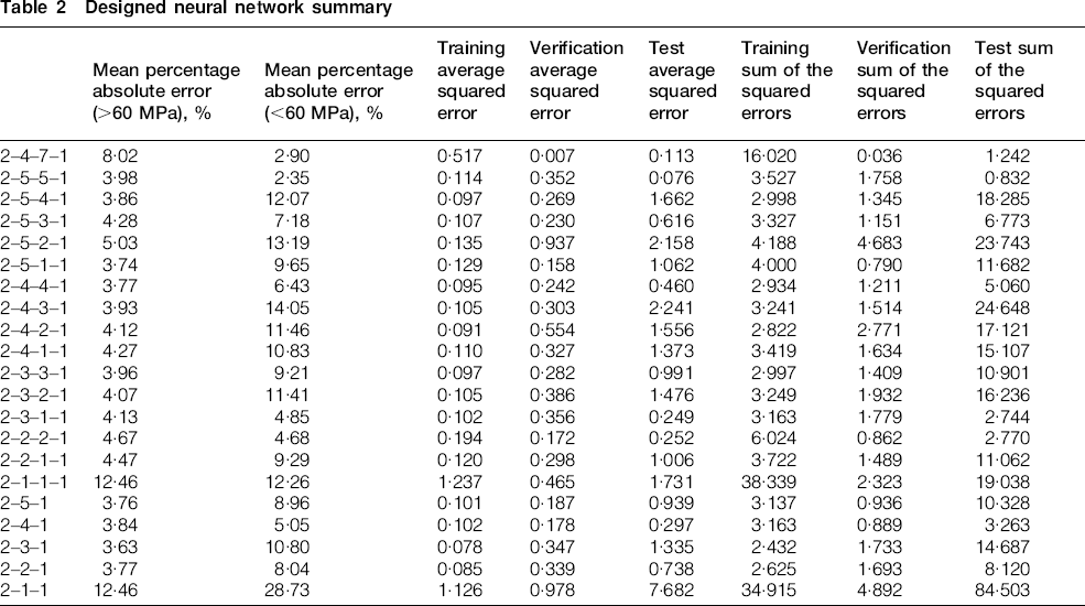
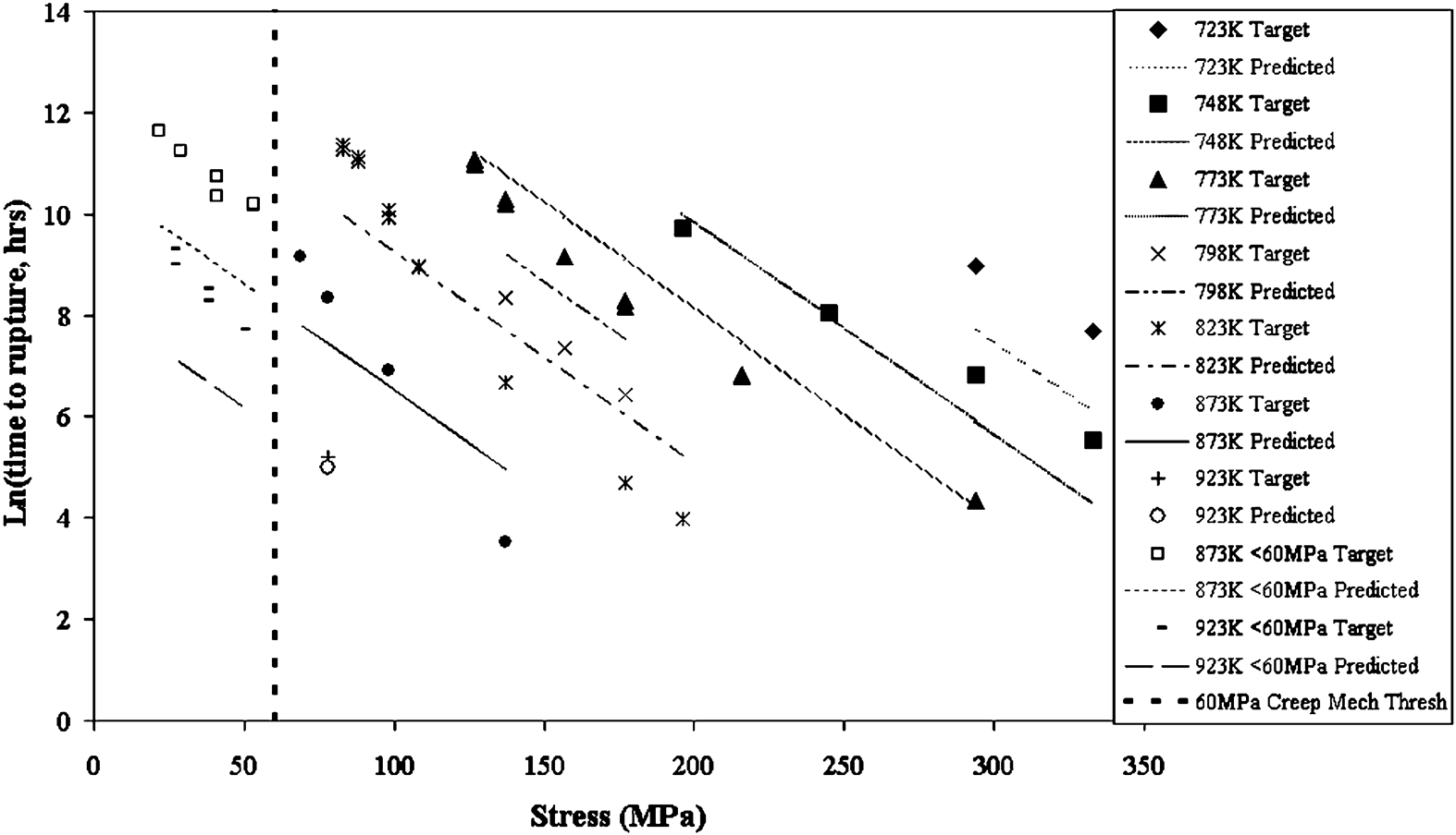
Table 2 shows that the 2–3–1 network has the lowest mean percentage absolute error above 60 MPa (3·63) but a high value for the stress range below 60 MPa (10·80). However, the 2–5–5–1 network has a marginally higher value for the stress range above 60 MPa (3·98) and the lowest value for the stress range below 60 MPa (2·35) of all the networks. The percentage error range below 60 MPa between the different networks ranges from 2·35 for the 2–5–5–1 network to 28·73 for the 2–1–1 network. The first network in the table (2–4–7–1) is the network created by the Auto-Designer function within the software. The errors in the predictions for this network are higher than many of the values for the personally designed networks. Figure 6 shows the values predicted by the 2–5–5–1 network plotted on the same graph as the experimental data.

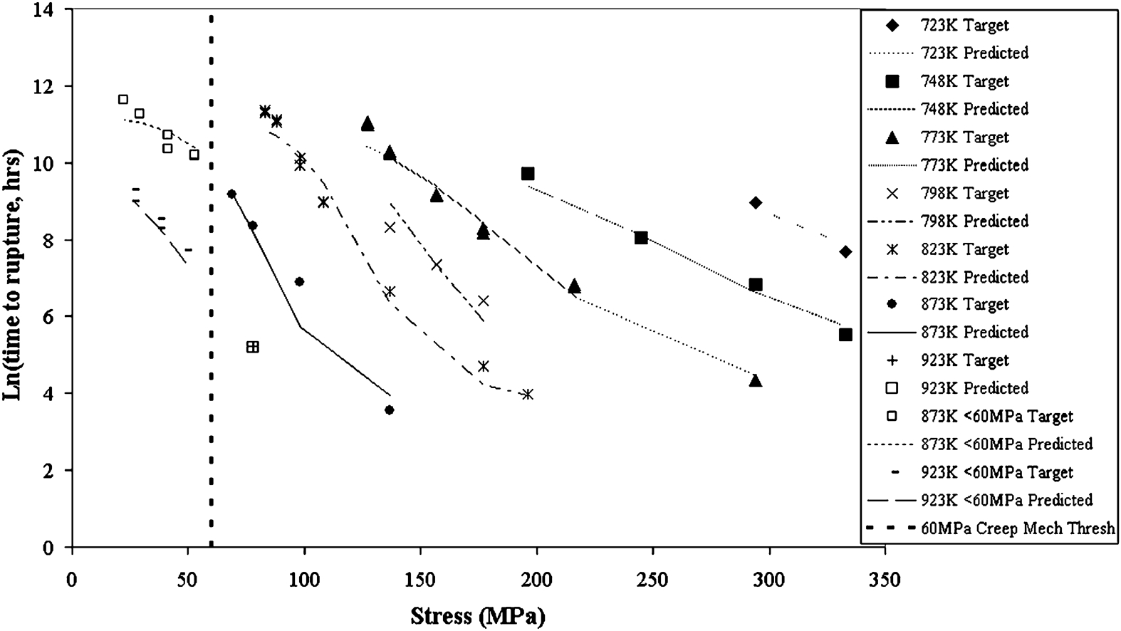
ln (time to rupture) v. stress for 2·25Cr–1Mo steel with outputs predicted by 2–5–5–1 neural network compared to actual measured data

Discussion

Parametric prediction

For the stress range below 60 MPa, the squared model has by far the lowest mean percentage absolute error (10·23) and is therefore the most accurate of the parametric models over this lower stress range at predicting the rupture life for a 2·25Cr–1Mo steel. For the stress range above 60 MPa, the cubic model has a slightly lower mean percentage absolute error (4·24 compared to 4·81 for the squared model) and is therefore the most accurate of the parametric models over this higher stress range at predicting the rupture life for a 2·25Cr–1Mo steel.

The above statement implies that there would be a conflict between the squared and cubic parametric models if only one was selected; therefore, a trade-off is required. First, the difference in the error over the higher stress range between the two models is very small (0·57); therefore, the squared model could be chosen without reducing the accuracy over this range significantly. Second, the difference in error over the lower stress range between the two models is relatively large (10·27); therefore, if the cubic model was chosen over this stress range, a significant decrease in the accuracy of the predictions would be observed. Finally, in this case, the function of the model is prediction of the long term rupture life of a component, where long term refers to the lower stress range; therefore, improved accuracy over the stress range below 60 MPa is of the greatest importance. Subsequently, for this application, the squared parametric model would be the optimum choice.

This work benefits from the advantage of having the experimental data for the lower stress range to compare with the predictions generated by the parametric model. If the parametric model was to be used to predict time to rupture values below 60 MPa and no experimental data were available for comparison at this stress level, the error in the higher stress range would be used in isolation to determine which parametric method is the most accurate. In this example, the cubic model was more accurate when compared with actual data over the higher stress range than either the squared or the linear models. Therefore, the cubic model would be selected as the model for predicting the long term rupture life, but this study found the cubic method to be less accurate than the squared model below 60 MPa. This is a critical flaw in creep rupture life predictions using the parametric model, as the accuracy at higher stresses is significantly different from the accuracy at lower stresses and could lead to overoptimistic predictions and dangerous, unexpected failures of boiler and heat exchanger tubes and pipes.

Neural network prediction

For the stress range below 60 MPa, the 2–5–5–1 network has the lowest mean percentage absolute error (2·35) and is therefore the most accurate of the network models generated at predicting the rupture life of a 2·25Cr–1Mo steel over the lower stress range. For the stress range above 60 MPa, nine networks have lower mean percentage absolute error values than the 2–5–5–1 network (3·98) with the 2–3–1 network having the lowest (3·63). The 2–3–1 network is therefore the most accurate network over the higher stress range at predicting the rupture life for a 2·25Cr–1Mo steel.

The same problem applies to the neural network models that applied to the parametric models, in that if the accuracy of the higher stress (short term) values was considered in isolation, then a network that provides less accurate lower stress (long term) predictions than other networks may be chosen, with the possibility of leading to overoptimistic predictions and premature failures of boiler and heat exchanger tubes and pipes. The difference between the lower stress level accuracy for the 2–5–5–1 and 2–3–1 network is 8·45 which is a large difference in comparison to the difference between the higher stress level accuracy (0·35). With the advantage of having the error values for both above and below 60 MPa, the 2–5–5–1 network is the optimum network for predicting the long term rupture life for a 2·25Cr–1Mo steel. The structure of the 2–5–5–1 network is shown in Fig. 7.

2–5–5–1 neural network, which produces most accurate predictions of creep rupture life at lower stresses

It is noted from the results that the ‘optimum’ network generated by the Auto-Designer (2–4–7–1) is different from the one found from the study (2–5–5–1), and it is also less accurate than this and many other networks generated in the study. This could be due to the weighting values and therefore, the predicted values vary because the starting values are dissimilar and training is then subsequently different.

Also, from the results, the 2–1–1 network has very high percentage absolute error values above and below 60 MPa. This could be attributed to the network only containing one hidden layer with one node, therefore producing a more simplistic neural network, similar to the parametric models.

Conclusions

The comparison between parametric models and neural networks and their relative suitability for predicting the long term creep rupture lives of 2·25Cr–1Mo steel has led to the following conclusions:

The cubic parametric model is the most accurate of the parametric models at predicting the shorter term (higher stress) creep rupture life, whereas the squared parametric model is the most accurate of the parametric models at predicting the long-term (lower stress) creep rupture life. In this case, the function of the model is prediction of the long term rupture life of a component; therefore, the squared model would be selected. Although, if the actual data below 60 MPa were not available for comparison with the predicted values, then the cubic model would be selected for its improved accuracy at higher stress levels. This could lead to dangerous overoptimistic predictions and unexpected failures of components at lower stress levels.

The 2–3–1 network is the most accurate of all the neural networks at predicting the shorter term (higher stress) creep rupture life but the 2–5–5–1 network is the most accurate of all the neural networks at predicting the long term (lower stress) creep rupture life. Again, in this case, the function of the model is prediction of the long term rupture life of a component; therefore the 2–5–5–1 network would be selected. If the actual data below 60 MPa were not available for comparison with the predicted values, then the 2–3–1 network would be selected for its improved accuracy at higher stress levels. This would result in a prediction that is not as accurate as it could potentially be via a neural network method, but provides a much greater level of accuracy compared to the parametric models for predictions below 60 MPa.

References

Ashby

M. F.

: Metall. Mater. Trans. A , 1983, 14A, 9, 1755–1769.

Ray

M. K.

, Sahay

S. K.

and Goswami

: Eng. Fail. Anal. , 2003, 10, (6), 645–654.

Raj

, Choudhary

B. K.

and Singh

R. K.

Raman: Int. J. Press. Vessels Pip. , 2004, 81, (6), 521–534.

Evans

R. W.

and Wilshire

: Proc. Sem. on ‘Design of high temperature metallic components’, 89–124; 1984, London, Elsevier Applied Science Publishers.

Evans

: Mater. Sci. , 2000, 35, (12), 2937–2948.

Monkman

F. C.

and Grant

N. J.

: Proc. ASTM , 1956, 56, 593.

Evans

: Mater. Sci. Technol. 1999, 15, (1), 91–100.

Manson

S. S.

and Haferd

A. M.

: ‘A linear time-temperature relation for extrapolation of creep and stress-rupture data’, Technical Note 2890, NASA, Washington, DC, USA, 1953.

Manson

S. S.

and Muraldihan

: ‘Analysis of creep rupture data in five multi heat alloys by minimum commitment method using double heat term centring techniques’, Research Project 638-1, EPRI Cs-3171, EPRI, Palo Alto, CA, USA, 1983.

10.

Trunin

I. I.

, Golobova

N. G.

and Loginov

E. A.

: Proc. 4th Int. Symp. on ‘Heat resistant metallic materials’, Mala Fatra, Czechoslovakia, September 1971, CSSR, 168.

11.

Larson

F. R.

and Miller

: Trans. ASME , 1952, 74, 765–775.

12.

Ray

A. K.

, Tiwari

Y. N.

, Sinha

R. K.

, Chaudhuri

and Singh

: Eng. Fail. Anal. , 2000, 7, (5), 359–376.

13.

Caubo

and Bragard

: ‘Heavy sheet for pressure vessels II – Heat resistance of A542 steel, Class 1’; 1980, Brussels, Commission of the European Communities.

14.

Azzam

: J. Aerosp. Eng., 1997, 211, (1), 29–38.

15.

Venkatesh

and Rack

H. J.

: Int. J. Fatigue , 1999, 21, (3), 225–234.

16.

Lee

J. A.

, Almond

D. P.

and Harris

: Composites A , 1999, 30A, (10), 1159–1169.

17.

Penny

R. K.

and Marriott

D. L.

: ‘Design for creep’, 205; 1995, London, Chapman & Hall.

18.

Swingler

: ‘Applying neural networks: a practical guide’, 3; 1996, London, Academic Press Ltd.

19.

Picton

: ‘Introduction to neural networks’, 21; 1994, London, Macmillan Press.

20.

Johnson

and Picton

: ‘Mechatronics, designing intelligent machines. Concepts in artificial intelligence’, 110; 1995, Oxford, Butterworth-Heinemann.

21.

Khanna

: ‘Foundations of neural networks’, 42; 1990, Boston, MA, Addison-Wesley.

22.

Hopgood

A. A.

: ’Knowledge-based systems for engineers and scientists’, 2nd edn, 199; 1993, New York, CRC Press.

23.

Smith

: ‘Neural networks for statistical modelling’, 43; 1993, New York, Van Nostrand Reinhold.

24.

National Research Institute for Metals : ‘NRIM creep data sheet’, No. 3B; 1986, Tsukuba, National Research Institute for Metals.

25.

Yamauchi

, Chuman

, Nishimura

and Masuyama

: ‘A study on Larson–Miller parameter constant for 2·25Cr–1Mo steel creep-rupture data’, in ‘Creep and fatigue: design and life assessment at high temperature’, 511–519; 1996, Bury St Edmunds, Mechanical Engineering Publications.