Joining of dissimilar metals: Issues and modelling techniques

Laser spot welding of dissimilar metals

The simplest case to analyse is that of a stationary spot weld using a laser, for which we can have a distinct process of melting during the application of the laser, followed by a solidification process after the laser is switched off. Dissimilar metals welding, however, is three-dimensional in nature even in a spot welding mode because of the asymmetry created by the difference in properties of the two metals being welded. Since the pieces of metal are initially separated in a butt welding arrangement, we have the option to model the melting process and mixing without having to consider the solidification process. It may be noted that any mixing of metals due to convection occurs only after the materials melts.

A schematic diagram of such a process corresponding to a Cu–Ni weld is shown in Fig. 1.2 Two pieces of copper and nickel are butt welded. Laser heat with a Gaussian distribution is applied symmetrically across the centreline of the butt joint. The Cu–Ni system chosen is very close to an ideal binary system with complete miscibility in liquid and solid states, and hence it justifies the mixture model assumption. The physical properties also vary according to the local concentration of the mixture, and are evaluated according to mixture theory. For properties of the mixtures, semiempirical correlations as functions of temperature and mass fraction are used.

OPEN IN VIEWER

Figure 1

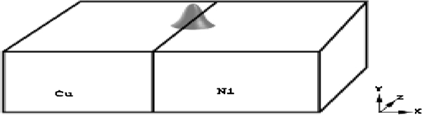
Schematic diagram of laser welding of Cu–Ni dissimilar couple2

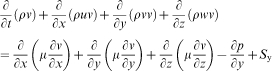
A single set of governing equations for the solid as well as liquid phases can be written using a single domain enthalpy porosity technique.10 The details of the governing equations consisting of continuity, momentum and energy conservation can be found elsewhere,11 and a brief representation of the set of equations is below:

Continuity: (1) Momentum: (2) (3) (4) Energy: (5) Mass fraction: (6) In the above equations, u, v, and w are the velocity components in the x, y, and z directions respectively, H is the enthalpy, C is the species concentration, μ is the dynamic viscosity, k is the thermal conductivity, D is mass diffusivity, and the S is the corresponding source term for the respective equations. The main assumptions made are that the weld pool surface is flat, the flow is laminar, incompressible, and driven by buoyancy and Marangoni forces, and the physical properties vary according to the concentration of the mixture. The standard enthalpy porosity technique for a melting problem is adapted to include the mixture enthalpy as (7) where H_Cu and H_Ni are the enthalpies of copper and nickel respectively, at a given temperature.

The results show that a symmetric application of laser heat along the centreline of the butt joint produces an asymmetric temperature distribution leading to an asymmetric pool development. This phenomenon is attributed to differential temperature rise because of difference in thermal diffusivities of the two metals. Interestingly, Nickel, melts first even though it has a higher melting temperature compared to copper, because of its lower thermal diffusivity. Another interesting fact revealed in Ref. 11 is that the temperature rises and melting of the copper side is enhanced by melt convection from the nickel half, in addition to direct laser heating. This is a unique contribution from modelling effort, as experiments alone could not have revealed these details.

Modelling of solidification during spot welding can be performed by switching of the laser power in the computational model. The solidification phenomena during the cooling stage are captured in Ref. 11. It is observed that the base metal (substrate) acts as a large heat sink for the small laser pool, hence the weld pool shrinks rapidly upon cooling. Also, the absence of laser heat on the weld pool weakens the Marangoni convection (as temperature gradients on the top surface are smaller), and hence fluid flow is mainly driven by natural convection at this stage. Very little mixing takes place during the solidification stage as the convection is weaker and the solidification is nearly instantaneous. Composition analysis of the solidified weld pool from numerical simulation reveals a good agreement with the corresponding experimental study,11 showing that a relatively simple model of melting and mixing is able to capture some significant details of spot laser welding of dissimilar metals.

Continuous laser welding of dissimilar metal welding

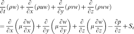
For the case of a continuous (or moving laser) welding process, modelling with respect to a fixed reference frame would require adjustment of grids continuously to maintain the grid concentration in and around the weld pool. It is a common practice in such situations to use a reference frame that is fixed to the laser. If the laser moves along the z-axis with a speed w_scan, the governing equations in the moving reference frame would remain the same as in the case of laser spot welding, except for additional source terms corresponding to the coordinate transformation.7, 8 The initial and boundary conditions remain the same as in spot welding except for the additional species mass flux conditions at the phase change interfaces. Figure 2 shows the top view and sectional view of the temperature contours and velocity profile of a snapshot of continuous weld between Cu–Ni.12 The asymmetry of the melt pool is clearly evident.

OPEN IN VIEWER

Figure 2

a top view and b sectional view of temperature contours and velocity profile of snapshot of Cu–Ni continuous weld12

The overall species balance and macrosegregation needs special attention in modelling of a continuous welding process as it involves a melting front and a solidification front. This will be discussed subsequently in more detail in the context of dissimilar gas metal arc welding (GMAW).

Laser welding of immiscible dissimilar molten metals

When dissimilar molten metals are immiscible (such as in monotectic systems), separate interfaces between the two metals exist within the pool, and one cannot use the simplified mixture principle to determine an average local concentration. One approach is to use a two-fluid model in which one formulates the problem with separate sets of governing equations for each metal. Such an approach is quite complex, as it involves the specification of interfacial terms for each conservation quantity, and coupling this with a phase change formulation (such as enthalpy approach) adds to the complexity. A more convenient approach is the volume of fluid (VOF) method,13 which can model two or more immiscible fluids by solving a single set of conservation equations and tracking the volume fraction of each of the fluids (or phases) throughout the domain. The VOF formulation relies on the fact that two or more fluids (or phases) are not interpenetrating. In each cell or control volume, the sum of the volume fractions of all phases is unity. The computational model tracks the volume fraction of each phase in each control volume, and the field variables and properties are shared by the phases and represent volume-averaged values. In the context of dissimilar metal welding, this concept has been successfully coupled with the enthalpy method by Chung and Wei14 to determine the interfaces between the immiscible dissimilar metals and between solid and liquid. In their simulations,14, 15 they used a VOF approach along with the SIMPLE algorithm16 to solve temperature, velocity and species distribution in the melt pool of a dissimilar joint using a two-dimensional transient formulation. Their computed results depict the transient velocity and temperature fields, the solute concentration on the free surface, and the shapes of the molten regions. The study illustrates the evolution of interface between the two melts during welding. However, details regarding solidification model and corresponding macrosegregation model were not available.

Another method suitable for modelling immiscible molten metal dissimilar weld is the level set method (LSM).17 In this context, a recent work on the application of level set method is reported by Tomashchuk et al., 18 in which LSM has been used to determine the position of the interface between immiscible components of a copper–stainless steel couple welded by electron beam. In the level set method, φ is a level-set function representing signed shortest distance to the interface. The variable φ can be convected by the fluid, and hence the complex interface morphologies between the two molten metals can be tracked by the solution of the level set function. The main advantage of LSM over VOF is the more accurate calculation of radius of curvature at the dissimilar metal interface. Interfacial tension between dissimilar melts can be modelled using the continuum surface force19 function, which requires an accurate estimation of the interfacial curvature.

Laser microjoining process

Transmission laser microjoining is a novel process where dissimilar and biocompatible materials can be joined, usually in lap geometry.20 The laser heat input in a Gaussian distribution is taken to be transmitted through the top layer (such as polyimide) and is absorbed on the surface of the bottom later (such as titanium). The issues concerning the optimisation of parameters are not those of mixing between the two layers but avoiding burning of the top layer. Good adhesion is obtained between the two layers when the top layer is not disintegrated and is only molten to react with the bottom layer to form a bond.21 Changes in thermophysical properties of the top layer due to phase change are to be considered for an accurate model. Addressing issues such as phase change and disintegration of the biocompatible materials under an intense heat source and their reaction with metallic materials are important for achieving better predictive capability.

Laser welding–brazing of dissimilar alloys

Brazing in inert atmosphere or vacuum is an established process to join dissimilar structural materials. Laser welding–brazing is a variant of laser welding technique where the filler material is fed to the V-groove of a butt joint. Since the braze joint involves a multicomponent alloy, a chemical potential based analysis is necessary to predict phase formation for good bond strength.22 For example, in a braze joint between titanium and eutectic Ag–Cu, saturation of the braze filler with Ti was observed to modify the sequence of phase formation significantly to lead to a successful joint.23 The multicomponent nature of a typical braze joint between dissimilar alloys poses challenges to the use of a simple solute balance equation to predict phase formation in the joint. Issues such as integration of computational thermodynamic databases with the heat transfer and fluid flow model at system scale need to be addressed.

GMAW of dissimilar alloy welds

The process of dissimilar materials welding can become even more complex in the case of GMAW, in which a filler material is added. The composition of the filler material may be different from those of the alloys that are welded. Filler material is introduced into the pool in the form of a molten electrode in either a ‘spray transfer’ mode or ‘droplet’ mode.24 This additional mode of heat and species addition to the pool can have a direct effect on the shape of the pool, along with temperature and concentration distribution within it.

A computational model simulating a GMAW process for joining dissimilar aluminium alloys was presented in Ref. 5. The model was presented with a case study of butt welding a plate of wrought aluminium alloy (Al–0·5 wt-%Si) to a plate of cast Al–Si alloy (Al–10 wt-%Si) using a GMAW process. The essence of the model was similar to the mixture model presented elsewhere.11 The addition of molten droplets from the filler rod (with a different composition) to the weld pool was simulated as volumetric heat and species sources distributed in an imaginary cylindrical cavity within the weld pool.25 A separate electrode thermal analysis was performed to determine the temperature (or enthalpy) and falling rate of molten metal from the electrode. Considering this dissimilar welding combination to form a binary system with the components being aluminium and silicon, a comprehensive model was developed to simulate melting, mixing, binary alloy solidification and macrosegregation in the molten zone as well as in the solidified weld region.

An important feature of model, especially from a metallurgical point of view, is the prediction of final species distribution in the solidified weld. Most weld pool simulations in the literature tend to focus on the heating, melting and convection in the molten pool. While convection simulation in the melt pool plays an important role in determining the weld pool shape and species distribution in the molten region, one still needs a suitable alloy solidification model along with appropriate microsegregation model (such as Scheil's model) to predict the solidified weld composition. It is revealed in Ref. 5 that the composition of the solidified alloy depends significantly on the solute distribution adjacent to the solidification interface. Appropriate species flux boundary conditions at the melting interface (i.e. at the leading edge of a moving weld pool), distributed species addition due to falling droplets, and species flux boundary conditions at the solidification interface (considering partitioning effects from the alloy phase diagram) must be specified for prediction of solidified weld composition.

Microscale modelling of dissimilar joining

Phase field modelling is an efficient diffuse interface approach to simulate microstructures taking thermodynamic and kinetic aspects into account.26 An application of this technique to microscale modelling of dissimilar welding show that the growth rate of crystals from the base material is not positive when there are strong compositional gradients ahead of the solid/liquid interface.27 These results corroborate the thermodynamic arguments to explain the difference in fusion line morphologies in most of the dissimilar metal combinations.2 It is known that sharp concentration gradients play a role in the nucleation of phases28 and thus are important in dissimilar welding.