Development of in situ measurement system for welding deformation using digital cameras

3D deformation time series measurement system

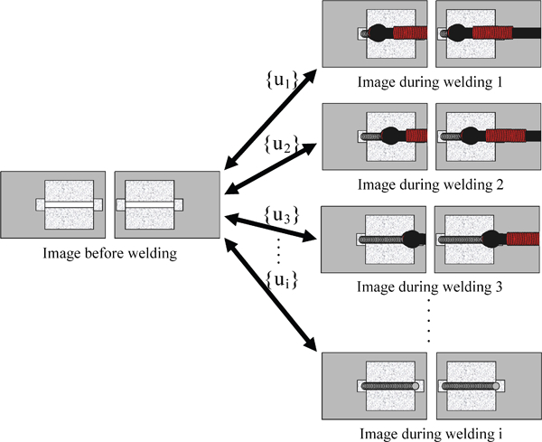
This system uses images captured sequentially before and during welding to calculate the amount of 3D deformation. An overview is shown in Fig. 1. First, two digital cameras are used to take photographs of the object before deformation. When the optical axes are parallel in the positional relationship of the two cameras and at the same time the camera angles around the optical axes are matched, the principles of stereoscopic imaging can be applied to calculate the 3D coordinates of the object. Then, the 3D shape of the measured object within an entire photographed region can be obtained by applying this method. In addition, the stereoscopic imaging necessitates correlating the locations in two images. This study uses the image correlation method,3^– 5 which is subpixel processed. By repeatedly applying this method to the time series images, the displacement from the prewelding pixel position in 3D coordinate can be obtained. Since the point of a given pixel position before deformation generally moves between pixels after deformation, the subpixel image correlation method is also applied to two images taken from the same camera (the left camera) before and after deformation. By comparing images from the same camera, it is possible to find the corresponding points before and after deformation.

OPEN IN VIEWER

Figure 1

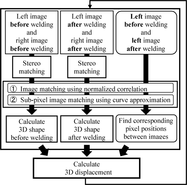
Flow of proposed measurement method

By repeating the above procedure from the start of welding until the end of cooling, full field time series measurement of 3D deformation, which is the objective of this research, can be achieved.

Fundamental principles of stereo imaging

Stereo imaging is a technique in which images of the same object are photographed from multiple viewpoints, and 3D coordinates of the object are acquired using the principle of triangulation from the parallax of the viewpoints. The binocular parallax method employed in this research is based on a particularly simple system configuration for stereo imaging systems, and so it has the advantage of few errors occurring from the camera parameters.

The binocular parallax method uses images photographed from two different directions, as shown in Fig. 2. In the figure, f is the focal length of the lenses, and B is the distance between cameras when the images are acquired. In this system, two cameras with equal focal lengths must be used. The cameras are positioned so that the y coordinate values are exactly the same for the same measurement point projected onto the left and right images, i.e. y_L = y_R. In addition, d is the parallax x_L−x_R, which is the shift in the projected positions from the left and right camera positions. Then, the 3D coordinates (X,Y,Z) are expressed by the following equations (1) (2) (3) Since the focal length f and the distance between each camera B are easily measured, the 3D coordinates can be found in the above equations by accurately seeking the corresponding points in the two images.

OPEN IN VIEWER

Figure 2

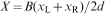
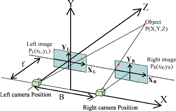
Illustration of binocular parallax

Image correlation method using normalised correlation

In this study, the amount of movement at each pixel point in two sequential images along the time history is calculated by the image matching method.6, 7 Specifically, the region with the highest similarity to a microregion in the reference image, which is the image before deformation, as shown in Fig. 3a, is detected in a comparison image, which is an image after deformation, as shown in Fig. 3b. The steps of this procedure are shown in the following:

OPEN IN VIEWER

Figure 3

Basic procedure of digital image correlation

i

a microregion dx×dy is set in the reference image and is centred at any given pixel position b_k(x₁,y_j). This region is defined as the subset region B(b_k)

ii

a subset region A(a_l), which corresponds to the microregion dx×dy, is similarly set in the comparison image and is centred at pixel position a_l(x₁+Δx,y_j+Δy). The brightness correlation value R(b_k,a_l) is calculated for B(b_k) and A(a_l)

iii

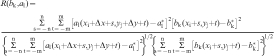
the brightness correlation value R(b_k,a_l) in the entire image area is found by shifting A(a_l) for every pixel. Numerous techniques have been proposed for evaluating the correlation between subset regions in the field of image matching, but a normalised correlation method8 was employed in this research by subtracting the average brightness value within the subset from the brightness value for each pixel when performing matching. This method is considered more robust to illumination changes, such as changes in the position or the light intensity of the light source, in comparison with methods such as the residual sum of squares correlation.3 The brightness correlation value R(b_k,a_l) in the normalised correlation is shown in the following equation (4) where 2n = dx−1, 2m = dy−1 and a* and b* indicate the average values of brightness within the subsets. Moreover, the closer the brightness correlation value R(b_k,a_l) is to 1, the higher is the correlation (i.e. the higher the similarity).

To obtain higher accuracy, the subpixel processing using curve approximation is adopted.

Total displacement and deformation measurement system

Figure 4 shows the flow of the total displacement and deformation measurement system employed in this research. In this technique, the total amount of displacement is directly found by performing image analysis between the images taken before deformation (i.e. before the start of welding) and 2N images, where N is the number of images taken by one camera throughout the welding until cooling is completed.

OPEN IN VIEWER

Figure 4

Total displacement type of measurement method

The accuracy of the total displacement and deformation measurement system is sensitive to the quality of the two images taken before deformation. However, since each image is handled independently during welding, the system has the advantage that, even if a measurement cannot be taken at some time interval, subsequent measurements are possible.

Experimental method and equipment

The experimental system for conducting the in situ measurement of welding deformation by the stereo imaging method is described in this section. Two cameras, two tripods and an aluminium beam are assembled as shown in Fig. 5 to photograph the test specimen straight on from the above. The 3D deformation of the test specimen is measured by taking images with each of the two cameras (left and right) for each time series. The test specimen was sprayed with a water based paint to provide a random pattern in order to increase the accuracy in image matching.

OPEN IN VIEWER

Figure 5

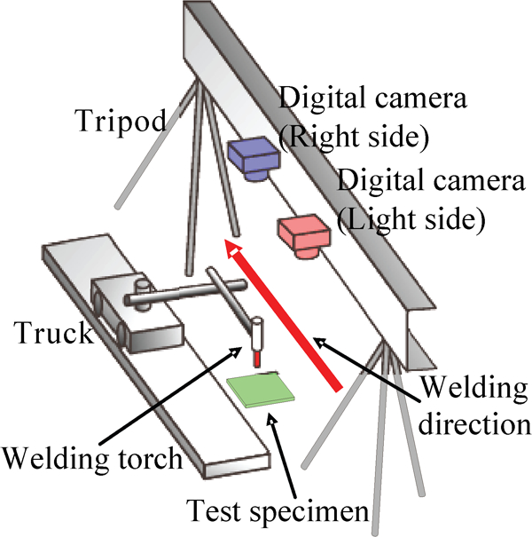
Experimental equipment

The dimensions of the test specimen are shown in Fig. 6. The test specimen was a plate 120 mm in length, 120 mm in width and 5·8 mm in thickness. The material used was SM490A. The welding torch was moved by using a constant velocity truck, so that heat was consistently applied from the welding torch to the test specimen. To set the boundary conditions as uniformly as possible, a jig was used to support the test specimen at three points from the underside so that the defused heat was relatively unrestrained from the front and back surfaces of the test specimen. Images were photographed at 5 s intervals with the left and right cameras synchronised. The resolution of the digital cameras used in the experiment was ∼15·1 million pixels, and the size per pixel in the photographed image was ∼62 μm. Additionally, the dimensions of the subset (shown in Fig. 3) were dx×dy = 20×20 pixels, which is approximately 1·25×1·25 mm. The welding current was 70 A, and the welding speed was 100 mm min⁻¹.

OPEN IN VIEWER

Figure 6

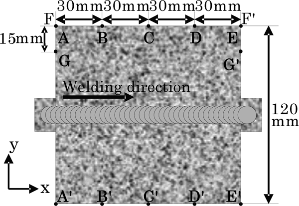
Shape and size of test specimen

Full field time series measurement of 3D deformation during welding

Images taken by the left camera during and after welding are shown in Fig. 7a. The displacement distributions in the x, y and z direction components are shown in Fig. 7b–d. In these figures, (i), (ii) and (iii) show the images captured and the displacement distributions at 30, 50 and 70 s after the start of welding respectively. Additionally, (iv) shows the distributions after cooling is complete. The images in Fig. 7a show that an area of intense light is associated with the arc light surrounding the welding torch. Additionally, in Fig. 7b, which is the x direction displacement distribution during welding, it is confirmed that a distribution of negative displacement is seen at the start point of the weld [1] (the bracketed numbers are shown in the figure), and a distribution of positive displacement is seen at the end point of the weld [2]. These distributions are caused by thermal expansion in the vicinity of the weld. It is also confirmed from the displacement distribution in the final deformation, shown in (iv) of Fig. 7b, that the heat transfer into the air is nearly complete, and the thermal expansion on the weld line during welding has nearly disappeared.

OPEN IN VIEWER

Figure 7

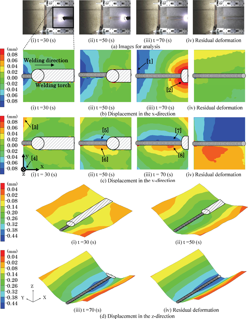
Distribution of displacements during welding, as measured by proposed method

It can be seen from the y direction displacement distribution at 30 s after the start of welding, shown in (i) of Fig. 7c, that the upper portion of the test specimen was displaced in the positive direction [3], while the lower portion of the test specimen was displaced in the negative direction [4]. This displacement is caused by thermal expansion in the y direction at the start point of the weld. The displacement distribution at 50 s after the start of welding, as shown in (ii), confirms that negative displacement was produced in the area [5] at the back of the torch, while positive displacement was produced in area [6]. It can be understood from this that localised thermal shrinkage occurs on the weld line in the transverse direction of the test specimen immediately after the welding torch passes. Local transverse thermal shrinkage [7] [8], as shown in (iii), immediately after passage of the welding torch, is similarly confirmed from the displacement distribution at 70 s after the start of welding. In addition, the residual deformation, as shown in (iv), confirms that the difference in displacement between the upper and lower portions of the test specimen, that is, the amount of transverse shrinkage, is greater at the end point than at the start point. Furthermore, from the distribution of displacement in the z direction, shown in d(i) and d(ii), angular distortion gradually forms from the location where the torch has passed. It can also be confirmed from the displacement distribution in (iii) and (iv) that virtually no change occurs in the resulting angular distortion after completion of welding, even with the passage of time.

The time history of the amount of transverse shrinkage is shown in Fig. 8. The vertical axis shows the amount of transverse shrinkage and the horizontal axis shows the passage of time from the start of welding. A–A′, B–B′, C–C′, D–D′ and E–E′ in the figure show the amounts of transverse shrinkage at positions 0, 30, 60, 90 and 120 mm respectively, in the direction of the weld line (Fig. 6). The amount of transverse shrinkage is defined as the amount of displacement in the y direction at points A, B, C, D and E minus the amount of displacement in the y direction at points A′, B′, C′, D′ and E′. It can be understood from these results that marked thermal expansion is observed when the heat source arrives near the starting and ending edges, which are A–A′ and E–E′. This is due to the fact that the constraint near the edges is larger than that inside the plate. It can also be confirmed that, as cooling proceeds, the shrinkage becomes greater as the end point of the weld becomes closer. One reason for this is that, since the welding speed is low when the torch is closer to the end point, the heat can accumulate due to the effects of thermal diffusion toward the end point.

OPEN IN VIEWER

Figure 8

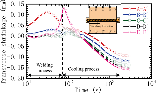
Time history of transverse shrinkage measured by proposed method

In Fig. 9, the time history of angular distortion is shown. A–A′, C–C′ and E–E′ in the figure show the time history of angular distortion at positions 0, 60 and 120 mm respectively from the start point of the weld (Fig. 6). From Fig. 9, it can be observed that angular distortion occurs immediately after the start of welding and progressively increases from the start point of the weld. It can also be confirmed that virtually no change occurs after welding is finished.

OPEN IN VIEWER

Figure 9

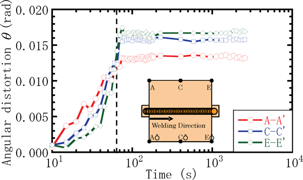
Time history of angular distortion measured by proposed method

These findings demonstrate that the proposed technique can acquire a smooth 3D displacement distribution across the full field measured area from the start of welding and throughout the cooling process.

Verification of accuracy after cooling is completed

In this section, the authors verify the accuracy of the results of the full field 3D deformation measurements obtained through the stereoscopic imaging method proposed in this research. First, round holes 2 mm in diameter were created at 27·5 mm intervals near the edges of the test specimen, as shown in Fig. 10. Then, digital calipers (instrumental error: ±0·02 mm) were used to measure the distance between each of the two holes shown at A–A′, B–B′, C–C′, D–D′ and E–E′ in Fig. 10 before welding and after welding. The validity of the in plane deformation measurements by the proposed method was verified by comparing the residual transverse shrinkage distribution measured by this caliper technique.

OPEN IN VIEWER

Figure 10

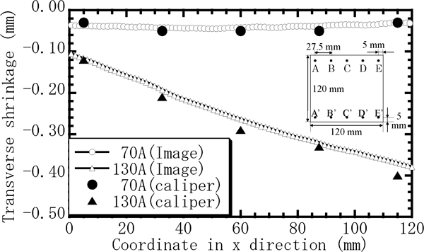
Distribution of transverse shrinkage

Figure 10 shows a comparison of the transverse shrinkage obtained by the proposed method and by the digital caliper measurements at currents of 70 and 130 A. The starting edge is shown at the left edge of the figure, and the end edge is shown at the right edge. These results show qualitative agreement between the measurements by the proposed method and by the digital calipers: the closer to the end edge, the greater the transverse shrinkage. It can also be seen that, in absolute values, the entire area from the start edge to the end edge can be measured with adequate accuracy for practical purposes using both methods, that is, with a maximum error of 0·02 mm, which is within the instrument error of digital calipers.

Next, to verify the accuracy of the out of plane deformation, a comparative study was conducted between the image measurements and the measurements by the laser displacement metre based 3D deformation measurement system (LAF-3D, guaranteed accuracy: 0·03 mm). Since the LAF-3D is a shape measurement system, not a deformation measurement system, and measures the coordinates of a physical surface, the deformation could not be strictly measured at the same locations as in the image measurement results, but it is presumed that it would be possible to measure nearly the same locations as long as the predeformation shape was flat and the in plane deformation was small. Figure 11 shows the image measurements of the out of plane deformation and the measurements by LAF-3D for currents 70 and 130 A. A relatively good quantitative match is found between the image measurements and the LAF-3D measurements.

OPEN IN VIEWER

Figure 11

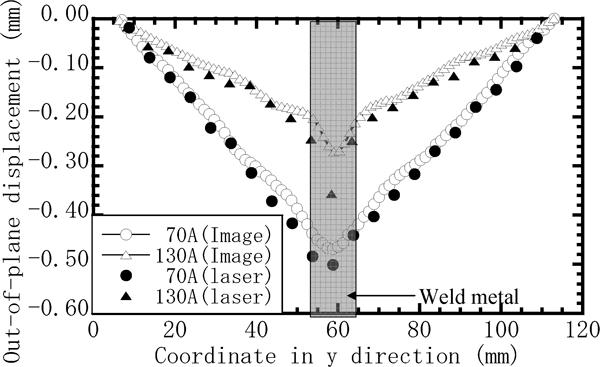
Distribution of out of plane displacement

The above results confirm that the proposed technique can be used to measure the deformation with good accuracy during welding, during the cooling process and after complete cooling. The proposed technique can be applied to the time series problem of 3D deformation over a wide range. For not only studying the mechanisms of welding deformation but also for quantitatively verifying the validity of FEM thermoelastic–plastic analyses, this technique is considered to be very promising.