Shear layer modelling for bobbin tool friction stir welding

Abstract

This study presents an approach to model the shear layer in bobbin tool friction stir welding. The proposed CFD model treats the material in the weld zone as a highly viscous non-Newtonian shear thinning liquid. A customised parametric solver is used to solve the highly non-linear Navier–Stokes equations. The contact state between tool and workpiece is determined by coupling the torque within the CFD model to a thermal pseudomechanical model. An existing analytic shear layer model is calibrated using artificial neural networks trained with the predictions of the CFD model. Validation experiments have been carried out using 4 mm thick sheets of AA 2024. The results show that the predicted torque and the shear layer shape are accurate. The combination of numerical and analytical modelling can reduce the computational effort significantly. It allows use of the calibrated analytic model inside an iterative process optimisation procedure.

Keywords

Friction stir welding Modelling Bobbin tool

Introduction

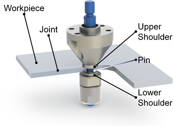
Friction stir welding (FSW) was developed and patented by Thomas et al. 1 It is a solid state joining process capable of welding a great number of materials, as pointed out by Mishra and Mahoney.2 The process is carried out by plunging a rotating tool into the workpiece and translating it along the weld line. The heat generated by friction at the tool surface and plastic dissipation soften the material to a plasticised state. It is then transported around the tool and consolidates to form a joint. The conventional tool design consists of a shoulder and a pin. Bobbin tools (also referred to as self-reacting tools) include a second shoulder attached to the end of the pin, as shown in Fig. 1.

Figure 1

Bobbin tool FSW (BT-FSW) process

These tools have some advantages over conventional tools, as pointed out by Hilgert et al. 3 As the z force acts only between the two shoulders in BT-FSW, the load carried by the welding machine is much smaller than in standard FSW. This allows for smaller and less rigid machines or robotic handling systems. As there is no need for a backing or anvil in BT-FSW, closed profiles like hollow extrusions can be joined. The microstructure of the joints is more symmetric as in standard FSW because of the symmetric tool.

The challenge in using bobbin tools is the high load acting on the pin. This load is difficult to determine. Experimental efforts are reported by Hattingh et al. 4 for standard FSW tools. Still, there is a knowledge gap when it comes to the interaction of bobbin tools with the welded material. In order to understand the loading on the tool and the formation of sound joints, the material flow in the shear layer around the tool needs to be known. Both can be investigated using numerical simulation.

The material flow around the pin of a FSW tool has been modelled in different ways. There is an approach by Heurtier et al. 5 that prescribes analytical velocity fields to determine stresses and strains of the welded material. The velocity fields are generated by superposition of circumventing, vortex and torsion velocity components. Although this is helpful to increase the understanding of the formation of different material flow patterns, it cannot be readily used in a predictive way for new process parameters. The most common approach in flow modelling of FSW is to solve a formulation of Navier–Stokes equations in a CFD framework.

Promising work has been published with focus on conventional FSW tools by several authors. First approaches include two-dimensional (2D) Eulerian models by Seidel and Reynolds,6 Schmidt7 and Colegrove and Shercliff.8 Some work has been extended to 3D models, as the one presented by Colegrove and Shercliff.9 Featured tools have been considered in a more recent work by Colegrove and Shercliff,10 Schmidt and Hattel11 and Atharifar et al. 12 An alternative approach to CFD models is CSM models. Recently, very good results have been obtained in that field by Guerdoux and Fourment.13 It has been shown by Arora et al. 14 that the torque acting during FSW can be predicted accurately by a material flow model.

It is possible to extend existing modelling methodologies for FSW to BT-FSW configuration. Deloison et al. 15 report on a 2·5D model of flow around a bobbin tool. The present study presents a 3D CFD model.

For process optimisation, a large number of solutions for different process parameters are needed. Therefore, there is a need for modelling techniques with a limited demand for computational resources. Usually, there is a tradeoff between solution time and solution detail. If fast and detailed solutions are needed, some measures are possible. A big gain in performance can be achieved when different physical interactions can be decoupled. The demand for computational resources can be further decreased when certain aspects of the process can be modelled analytically instead of numerically. The approach presented in this study is to use an analytical shear layer model (ASLM) that was presented by Hilgert et al. 3 as part of a thermal pseudomechanical (TPM) model for BT-FSW. The input parameters for the ASLM are predicted by an artificial neural network (ANN) trained with numerical predictions of the CFD model.

Model

CFD model

A CFD model is implemented in Comsol Multiphysics. The geometry (Fig. 2) consists of a part of the base material sheet. The tool pin is cut out of the plate. The tool shoulders are imprinted as boundaries on the top and bottom surfaces of the workpiece. The domain of the plate is chosen sufficiently large so that the material flow on both the inlet and the outlet surfaces is parallel to the welding direction and has the same velocity as the nominal welding speed. This means that any softening and stirring in the vicinity of the pin and shoulders are captured within the modelled domain. The material at the outer boundaries can be considered solid. It has a finite but very high viscosity.

Figure 2

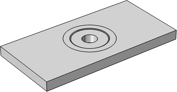
Geometry of flow model

Equations

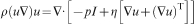
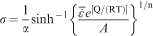
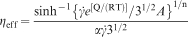
The governing equation is the Navier–Stokes equation, as expressed in equations (1) and (2) (1) (2) where u is the velocity vector, and η is the viscosity.

The viscosity is defined using the inverse hyperbolic sine law, as suggested by Aukrust and LaZghab16 for material flow stress. It is a function of temperature and shear rate. The standard form in terms of effective deviatoric flow stress and effective strain rate is given in equation (3). This needs to be converted to a system of effective viscosity η_eff and shear rate for flow modelling, i.e. (3) (4) (5) (6) Here, R is the universal gas constant, and α, A, Q and n are material properties. For the alloy AA 2024, these constants are taken from Sheppard17 and are given in Table 1.

Table 1

Material parameters for AA 202417

Parameter	Value
α/m² N⁻¹	1·6×10⁻⁸
A/s⁻¹	e ^19·6
Q/J mol⁻¹	1·4880×10⁵
n	4·27

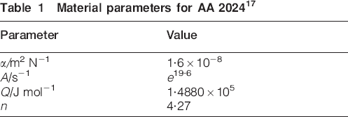
The resulting effective viscosity η_eff for the range of temperature and shear rate of interest in this context is shown in Fig. 3.

Figure 3

Effective viscosity η_eff (IHSL)

As the viscosity is described by a very non-linear function, a parametric solver approach can help to achieve convergence. Hereby, the effective viscosity is increased using a convergence parameter n_conv going from 10 to 1, according to equation (7). The necessity of this approach as well as the selection of the range of the convergence factor depends on the solver settings and the complexity of the geometry under investigation, i.e. (7)

Boundary conditions

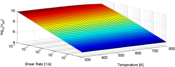
Figure 4 shows the different boundary groups of the CFD model.

Figure 4

CFD model boundary conditions

The boundary conditions of the inlet surface (Fig. 4a) define a constant material flow velocity in the welding direction. The same is true for the side walls, as shown in Fig. 4d. This represents the actual behaviour of the material, which does not deform outside a small shear layer around the tool. The outlet surface (Fig. 4b) prescribes a constant relative pressure of zero. The free surface (Fig. 4c) of the plate is set to have a slip condition (u.n = 0) so that no material can leave the plate. The pin and shoulder surfaces (Fig. 4e) prescribe a defined tangential velocity v_tangent compatible with the tool's rotation speed ω according to equation (8) (8) where, r is the distance from the tool axis, ω is the tool angular velocity and δ is the contact state variable (0<δ<1) that defines the ratio of sticking and slipping at the interface, as described by Schmidt and Hattel. 18 18,19

Predictions

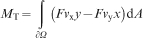
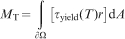
The torque M_T acting in the pin can be calculated according to equation (9) (9) where Fv is the viscous force per area acting on a location on the pin surface, and x and y are the distances from the tool axis.

The contact condition is difficult to determine experimentally. It can, however, be predicted by the CFD model, as shown by Nandan et al. 20 In the present study, this is performed by prescribing a global constraint to the torque variable in the CFD model. The correct value is predicted by the TPM model and validated experimentally. This way, the contact state variable δ can be solved for as an additional degree of freedom during the solution of the model.

Temperature and torque

The temperature fields and torque values used in the CFD model are predicted by a thermal model presented by Hilgert et al. 3 There, the experimental validation of the thermal predictions is also presented. The model uses a TPM heat source defined in equation (10), as proposed by Schmidt and Hattel.18 Therefore, the only a priori unknown input parameter is the material property shear yield stress, which is a function of temperature. Once these data are found experimentally, no further calibration is needed when changing other process parameters like welding speed, tool rotational speed or plate thickness (10) A unique capability of the TPM heat source is to predict the machine torque from a numerical simulation with only thermal degrees of freedom. This is performed by integrating the temperature dependent material flow stress τ_yield(T) multiplied with the distance from the rotational axis of the tool r over the contact surface of the tool and the workpiece according to equation (11). This assumes the stresses to be in tangential direction only, which has to be taken into account when working with complex geometry features on the pin (11)

Analytic shear layer model

In order to correctly predict the thermal field in the TPM model, a convective heat flux representing the material flow in the shear layer around the tool is included. With such a shear layer model, the inherent asymmetry of the FSW process can be captured. In this study, the ASLM that was described along with the TPM model by Hilgert et al. 3 is calibrated. The equations are based on previous work by Schmidt and Hattel21 on conventional FSW tool shear layers. The ASLM defines a velocity field in close vicinity of the tool. This velocity is used to generate the convective heat flux resembling the material moved around the tool. The model uses a coordinate system based on r and z directions, as the shear layer is simplified to be axisymmetric. The formulation of the ASLM guarantees continuity at the interface between the tool and the workpiece. The shape and velocity profile are defined by four parameters m_shape, m_r, m_z and R_m that need to be calibrated.

Here, m_shape controls the slope of the outer contour of the shear layer that corresponds to the boundary of the thermomechanically affected zone and the heat affected zone in a cross-section. Higher values result in a shear layer shape with a more pronounced influence of the shoulder. The parameters m_r and m_z govern the slope of the shear layer velocity in the radial and thickness directions. Higher values result in increasing velocity gradient. R_m governs the minimal diameter of the shear layer in the centre of the workpiece.

Calibration with ANN

The ASLM is designed to save computational time. It is meant to eliminate the need for CFD calculations for every set of new process parameters. Therefore, the input parameters need to be determined in a fast but reliable way. In this study, an ANN is trained with the predictions of the CFD model for a set of process parameter combinations. The well trained ANN is then used to predict the ASLM parameters with marginal computational effort.

The ANN used for this purpose is composed of an input layer, two hidden layers and an output layer. The input layer consists of two neurons representing the process parameters welding speed and tool rotational speed, as these are the controlling parameters of the CFD model. The hidden layers consist of three neurons each. The output layer consists of four output neurons representing the calibration parameters for the ASLM, i.e. m_shape, m_r, m_z and R_m. The topology is plotted in Fig. 5. The neural weights are indicated by the colour of the neural connections, where red indicates a small (negative) weight, and green indicates a high weight.

Figure 5

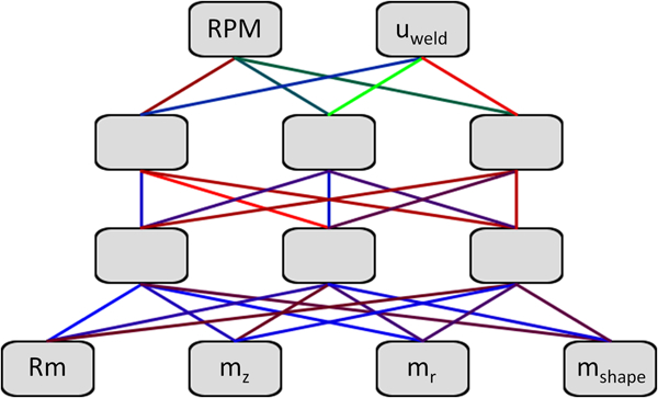
Topology of ANN

The training patterns are created by fitting the parameters of the ASLM to the flow field predictions of the CFD model at the retreating side of the weld. The fitting is performed using non-linear minimisation capabilities from Matlab's Optimisation Toolbox.

Of course, the prediction of the ASLM is only an approximation of the actual shape and velocity profile of the material flow around the tool. The true material flow is not axisymmetic but has a pronounced difference between the retreating and advancing sides. It has to be emphasised that calibration of the ASLM is performed from steady state solutions of flow around tools with simplified geometry. This is, however, sufficient to accurately reproduce the temperature difference between the advancing and retreating sides in the far field of the temperature distribution.

Experimental

The shape and size of the predicted shear layer as well as the torque M_T that is predicted by the thermal model and used by the CFD model have been validated experimentally. The material used is a sheet of 4 mm thick aluminium alloy 2024 in T351 condition. It is welded using a bobbin tool with 8 mm pin and 15 mm scrolled shoulders, as shown in Fig. 1.

Results and discussion

An example of the velocity field predicted by the CFD model is given in Fig. 6.

Figure 6

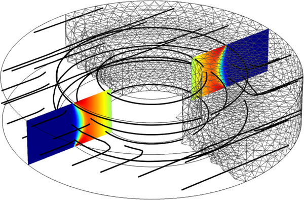
Predicted flow velocity profile

The material flow velocity profile at the retreating side is used to calibrate the ASLM. The velocity profile predicted with the CFD model is compared to the macrograph of an experimental weld in Fig. 7. After welding, a sample is taken from the joint and polished and etched with Keller's solution to reveal the shear layer shape.

Figure 7

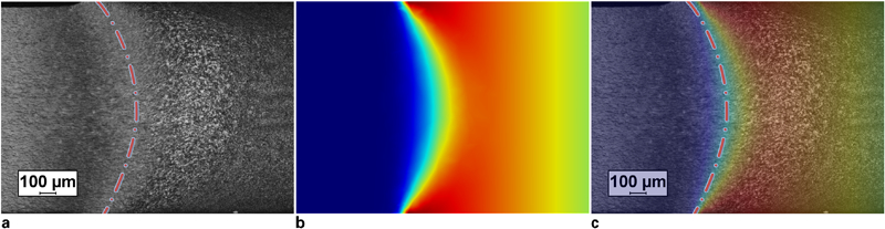
Comparison between predicted shear layer (red colour indicates high velocity) and microstructure

The comparison is based on the assumption that the boundary between the thermomechanically affected zone and the heat affected zone of the microstructure corresponds to the maximum extent of the shear layer during welding. This boundary can be empirically found on the etched macrograph by comparing the microstructure to the base material microstructure. Areas that show signs of deformation, reorientation or recrystallisation are attributed to the shear layer.

The prediction shows good agreement in shear layer shape. The absolute value of the predicted shear layer velocity is not easy to validate experimentally. New experiments based on marker material investigation need to be developed.

An ANN was trained with a total of 64 data patterns generated from CFD results. The process parameters reach from 400 to 1200 rev min⁻¹ for the tool rotation and from 0·5 to 5 mm s⁻¹ for the welding speed. The training algorithm used was resilient backpropagation.

The comparison between trained and predicted values is plotted in Fig. 8. The blue circles correspond to a pattern that has been used for training. The red circles correspond to validation patterns that have not been used for training. Figure 9 shows the predictions for the shear layer parameter fields.

Figure 8

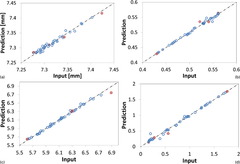
Comparison between trained and predicted values for shear layer parameters a R_m, b m_z, c m_r and d m_shape

Figure 9

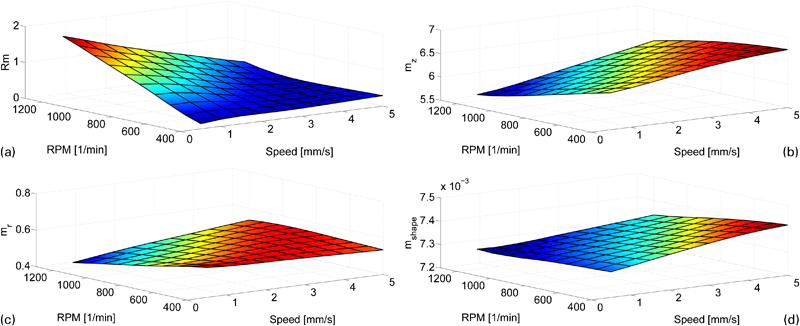
Predicted values for shear layer parameters a R_m, b m_z, c m_r and d m_shape

The trained ANN is able to predict the optimal inputs for the ASLM with adequate precision. The valid range of predictions can be extended by generating more training patterns with the CFD model in the desired region of the parameter space.

As described above, the TPM heat source can be used to predict the acting torque on the tool from the resolved shear stresses on the tool surface. A series of predictions for welds with 600 rev min⁻¹ are shown in Fig. 10 together with experimental validation data derived from measurements of spindle motor current and voltage.

Figure 10

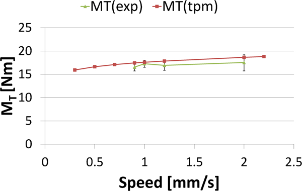
Predictions for torque

The predictions are sufficiently accurate to be used in the CFD model.

Of course, equation (8) includes the assumption that the same contact state is present at all interfaces between tool and workpiece. This is a common assumption in the literature, e.g. by Schmidt and Hattel22 and Colegrove and Shercliff.23 Still, it may well be possible to find different contact states at the pin and shoulders of the tool. This cannot be taken into account using the methods described here.

The geometry is kept simple and does not include details of the shoulder and pin. This approximation gives reasonable results for simple tools. Featured tools can be dealt with in a similar manner, as demonstrated by Schmidt and Hattel,24 but the computational cost makes parameter studies slow and resource demanding. Additionally, it has to be stated that this only applies to a steady state approximation of a featured tool. The CFD model presented here has been extended to include transient rotating featured tools. Details will be published separately.

The TPM model uses material data as an input for τ. These data are considered to be a function of temperature only. It has been shown that very good results can be achieved in this way. Still, improvements seem possible when including the shear rate known from CFD results into the TPM equation. This is the subject of continuing work.

Conclusions

A 3D CFD model of the material flow around a bobbin tool is presented. The predicted shape of the shear layer is found to be in good agreement with experimental observations. The contact state δ between the tool and the joined material is part of the predictions rather than necessary input of the model.

In order to achieve fast predictions, an ASLM can be calibrated with predictions of this CFD model. The calibration is achieved with small computational cost using an ANN. This ANN is trained with CFD predictions for different process parameter sets. It has been shown that ANN is capable of predicting the input parameters of the ASLM for new sets of process parameters with good accuracy. This combination of numerical and analytical methods allows for process modelling in BT-FSW with high accuracy and low computational time. The TPM model with calibrated ASLM can be used in iterative process development cycles due to its low computational cost. It allows for accurate prediction of temperature and torque while solving for thermal degrees of freedom only.

It has to be emphasised, though, that this mixed approach is designed for fast predictions only. A deeper insight into the physics of the problem can only be gained through the 3D coupled thermomechanical model.

References

Thomas

, Nicholas

, Needham

, Murch

, Templesmith

, Dawes

: ‘Friction stir welding’, GB 9125978·8, 1991.

Mishra

, Mahoney

, (ed.): ‘Friction stir welding and processing’; 2007, Materials Park, OH, ASM International.

Hilgert

, Schmidt

, dos Santos

, Huber

: J. Mater. Process. Technol., 2010, 211, (2), 197–204.

Hattingh

, Blignault

, van Niekerk

, James

: J. Mater. Process. Technol., 2008, 203, (1–3), 46–57.

Heurtier

, Jones

, Desrayaud

, Driver

, Montheillet

, Allehaux

: J. Mater. Process. Technol., 2006, 171, (3), 348–357.

Seidel

, Reynolds

: Sci. Technol. Weld. Join., 2003, 8, 175–183.

Schmidt

: ‘Modelling the thermomechanical conditions in friction stir welding’, PhD thesis, Department of Manufacturing Engineering and Management, Technical University of Denmark, Lyngby, Denmark, 2004.

Colegrove

, Shercliff

: Sci. Technol. Weld. Join., 2004, 9, 483–492.

Colegrove

, Shercliff

: Sci. Technol. Weld. Join., 2003, 8, 360–368.

10.

Colegrove

, Shercliff

: J. Mater. Process. Technol., 2005, 169, 320–327.

11.

Schmidt

, Hattel

: Proc. COMSOL Conf., Hannover, Germany, November 2008, COMSOL. Paper no. 141.

12.

Atharifar

, Lin

, Kovacevic

: J. Mater. Eng. Perform., 2009, 18, (4), 339–350.

13.

Guerdoux

, Fourment

: Modell. Simul. Mater. Sci. Eng., 2009, 17, (7), 075001.

14.

Arora

, Nandan

, Reynolds

, DebRoy

: ‘Torque, power requirement and stir zone geometry in friction stir welding through modeling and experiments’, Scr. Mater., 2009, 60, 13–16.

15.

Deloison

, Jacquin

, Gurin

, Desrayaud

, Marie

: Proc. 3rd FSW Modelling and Material Flow Visualisation Sem., Geesthacht, Germany, April 2008, GKSS, 122–149.

16.

Aukrust

, LaZghab

: Int. J. Plast., 2000, 16, (1), 59–71.

17.

Sheppard

: Mater. Sci. Technol., 1993, 9, (11), 430–440.

18.

Schmidt

, Hattel

: Scr. Mater., 2008, 58, (5), 332–337.

19.

Schmidt

, Hattel

: Int. J. Offshore Polar Eng., 2004, 14, (4), 294–304.

20.

Nandan

, Roy

, Lienert

, DebRoy

: ‘Three dimensional heat and material flow during friction stir welding of mild steel’, Acta Mater., 2007, 55, (3), 883–895.

21.

Schmidt

, Hattel

: Sci. Technol. Weld. Join., 2005, 10, (2), 167–186.

22.

Schmidt

, Hattel

: Modell. Simul. Mater. Sci. Eng., 2005, 13, 77–93.

23.

Colegrove

, Shercliff

: Sci. Technol. Weld. Join., 2006, 11, (13), 429–441.

24.

Schmidt

, Hattel

: Proc. 7th Int. Symp. on ‘Friction stir welding’, Awaji Island, Japan, May 2008, TWI.