
Abstract
Many finite element models use adjustable parameters that control the heat loss to the backing bar, as well as the heat input to the weld. In this paper, we describe a method for determining these parameters with a hybrid artificial neural network (ANN) coupled thermal flow process model of the friction stir welding process. The method successfully determined temperature dependent boundary condition parameters for a series of friction stir welds in 3·2 mm thick 7449 aluminium alloy. The success of the technique depended on the method used to input thermal data into the ANN and the ANN topology. Using this technique to obtain the adjustable parameters of a model is more efficient than the conventional trial and error approach, especially where complex boundary conditions are implemented.
Keywords
Introduction
In friction stir welding (FSW) modelling, two major approaches have been used to describe the heat loss from the workpiece to the backing bar. The first method simplifies the heat loss using a convective transfer and has been used by Khandkar et al., 1 Nandan et al. 2 and Arora et al. 3 The second method uses a contact gap conductance to represent the imperfect contact at the interface between the workpiece and the backing bar.1, 4, 5 The contact gap conductance k is defined as k = Q/(T0−TA), where Q is the heat flux from the workpiece to the backing bar, T0 is the temperature of the workpiece and TA is the temperature of the backing bar. Khandkar et al. 1 found that using the contact gap conductance method was more accurate than the convective heat transfer coefficient. Simar et al., 4 Colegrove et al. 5 and Shi et al. 6 have used a variable contact gap conductance in their models. Shi et al. 6 applied a temperature dependent contact gap conductance method where the value increased with temperature to simulate the better contact under the tool.
Process models can be linked to artificial neural network (ANN) models to find the unknown boundary coefficients. Such models have been called ‘hybrid models’ due to the combination of the two model types. Sablani7 and Sreekanth et al. 8 have applied similar concepts in their analysis of the heat transfer between the solid particles and a fluid. The general procedure for developing a hybrid model is:7
obtaining a group of temperature versus time curves from analytic or numerical thermal models using different boundary conditions
training the ANN model using the outputs from the thermal model as inputs, while using the boundary condition inputs of the thermal model as outputs to the ANN model
inputting experimental thermal data into the trained ANN to find the corresponding boundary conditions, once the ANN has been trained.
Artificial neural network models have also been applied to welding processes.9 The main purpose of this study is to investigate the thermal boundary conditions using a hybrid model of the FSW process. This will be applied to a series of welds produced with the ‘Flexi-Stir’ FSW machine, which is used to analyse the phase changes that occur during welding with synchrotron radiation. The study investigates different methods for inputting the thermal data into the ANN as well as different ANN topologies.
Friction stir welding experiments
The experimental FSW work was performed on 3·2 mm thick 7449-T7 plates at Helmholtz-Zentrum Geesthacht. The length of the plate was 250 mm, and the width was 150 mm. The tool shoulder was flat with a scroll feature, and its radius is 6·5 mm. The threaded triflat pin had a radius at the top of 2·5 mm and tip radius of 1·9 mm, with an overall length of 3·2 mm. The tool tilt angle was 3°. The ‘Flexi-Stir’ machine10 developed at Helmholtz-Zentrum Geesthacht used two backing bars: a 1 mm thick, 19 mm wide copper backing bar underneath the workpiece that was supported by two steel blocks (geometries as shown in Fig. 1). A 3 mm gap was provided between the steel blocks underneath the copper backing bar. The thin copper backing bar underneath the tool allowed the synchrotron radiation to pass through the workpiece to the target while providing minimal support to the underside of the weld. The copper backing bar deformed during processing; the support provided with this set-up is much poorer than that provided by a conventional backing bar. Nevertheless, good thermal contact is maintained throughout: the workpiece and the copper backing deformed together during welding. In addition, the workpieces were clamped to the steel blocks, and the copper bar was correspondingly clamped in between the workpiece and the steel blocks.

Diagram of geometry used for process model
Travel speeds of 2, 3, 4, 5, 6 and 8 mm s−1 with a rotation speed of 1300 rev min−1 were used for the welds. K type thermocouples were used for measuring the thermal profile. The thermocouples were positioned 8±0·5, 13±0·5 and 18±0·5 mm away from the centre of the weld. They were inserted into 1·6±0·1 mm deep, ø1 mm holes, and a polysynthetic silver thermal compound (including aluminium and zinc oxides particles) was applied to aid heat transfer between the thermocouple and the workpiece material. Thermal tape was used to hold the thermocouples in position. The actual position of the thermocouples was validated by measuring the distance from the centreline on the weld macrosections. The thermocouple at 8 mm away from the weld centre was within the heat affected zone but close to the thermomechanically affected zone (TMAZ) boundary for the 3 mm s−1 travel speed weld. As the travel speed increased, the distance to the TMAZ boundary increased. Therefore, all the thermocouples were sufficiently far from the TMAZ so their position was not affected by the welding process. This enabled direct comparison with the temperature measurements from the numerical model. The thermal profiles from the retreating and advancing sides were averaged before inputting into the ANN model. The average temperature difference between the advancing and retreating sides was measured to be 13°C. The welds were completed with position control. The Flexi-Stir machine did not allow measurement of either the axial load or the torque.
Hybrid model development
Structure of hybrid model
The hybrid modelling procedure consists of the following steps:
applying several groups of hypothetical boundary condition values to the FSW process model and obtain the corresponding thermal data
abstracting or summarising the thermal data so that the characteristics of the thermal curves can be represented by key data values
training the ANN models with the data values from step 2; note that during training, the thermal data are inputs and the boundary condition values are outputs
abstracting the experimental thermal data using the same method that was used for the model data and input into the trained ANN; obtaining the predicted boundary condition values
enter the predicted boundary conditions into the FSW process model and obtain the corresponding thermal data
comparing the predicted thermal data with experimental thermal data.
Friction stir welding process model
The FSW process model is a three-dimensional fully coupled model developed with FLUENT CFD solver and is similar to that described by Colegrove et al. 5 The model was solved in the steady state mode, which was found suitable for all travel speeds according to the procedure described by Grong.11 This strategy resulted in a more rapid solution than a full transient simulation.
The geometry of the model is given in Fig. 1. The overall geometry of the tool was described previously. The profiled features on the shoulder (scroll) and the pin (threads and flats) were ignored to simplify the mesh generation: the shoulder was modelled as an annulus and the pin as a truncated cone. In addition, the tool tilt was not included in the model. In models where the material sticks to the surface of the tool, such as the one presented in this paper, the effect of the tool features on the heat generation is minimal.12 Ignoring the features on the tool is a common simplification in FSW process models.1, 4
In the flow model, the Navier–Stokes equation13 is solved. The material viscosity is found from the following relationship12

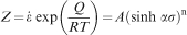
 is the effective strain rate. The material flow stress was calculated from a modified version of Zener–Holloman law proposed by Sellars and Tegart,14 which is widely used for aluminium alloys.15,
16 The Zener–Holloman equation is given by
is the effective strain rate. The material flow stress was calculated from a modified version of Zener–Holloman law proposed by Sellars and Tegart,14 which is widely used for aluminium alloys.15,
16 The Zener–Holloman equation is given by
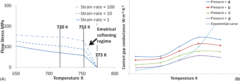
(A) material flow stress as function of temperature and strain rate for 7449-T7 aluminium alloy17 and (B) schematic plot of contact gap conductance versus temperature and pressure based on values from Zhu et al. 21 (note pressure values from large to small are a–d, and numerical values for axis are not included due to copyright consideration)
Constitutive constants for 7449-T7

A sticking condition was assumed between the workpiece material and the tool. Full contact between the shoulder of the tool and the workpiece material was not used. During FSW, the shoulder is often not in full contact with the workpiece material because there is often a loss of contact along the front edge due to the tilt angle. In addition, there may be some slip between the tool and the workpiece material in the real weld. One way of dealing with these issues involves applying a reduced shoulder contact radius.5 Hence, the sticking condition was only applied to the reduced shoulder contact radius, and the contact shoulder radius ratio (CSRR) was defined as the ratio of the contact shoulder radius to the original radius of the tool. Since the shoulder contact radius has a direct impact on the heat generation, it is one of the adjustable parameters in the hybrid model.
Since the material movement away from the welding tool is negligible, the workpiece was divided into a liquid-like aluminium region beside the tool in which the momentum and heat equations were solved, and a solid aluminium region in the far field in which only the heat equation was solved.
The heat equation was solved in the thermal model.18 The flow stress and strain rate from the flow model were used to calculate the viscous heat generation from the following equation13


The main difference between this model and the one reported by Colegrove et al.
5 is the thermal boundary conditions due to the unique design of the machine. To model the imperfect contact between the aluminium workpiece and the backing bars, temperature dependent contact gap conductance boundary conditions were applied. As shown in Fig. 1, there are three interfacial boundaries that need to be determined: the boundary condition between the aluminium workpiece and the copper backing bar k1, the aluminium workpiece and the steel backing bar k2 and between the copper and steel backing bars k3. An experimental investigation of the contact gap conductance by Yüncü19 showed that the values between aluminium and steel, and copper and steel were similar and approximately a quarter of the value between copper and aluminium. As stated in the ‘Introduction’ section, temperature dependent contact gap conductance between the aluminium workpiece and steel backing bar was used by Shi et al.
6 and Rohsenow and Hartnett.20 Although discrete values in the form of a lookup table were used, the values approximate an exponential curve. The justification for this approach can be seen in the schematic plot of contact conductance versus temperature and pressure based on the experimental results from Zhu et al.
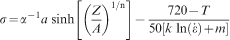
21 in Fig. 2B. In the far field, both the temperature and interfacial pressure are low, which leads to a low contact gap conductance. Near the tool, both the temperature and pressure increase, leading to an exponential increase in the contact gap conductance with temperature (if the pressure is not included as a parameter). Therefore, the temperature dependent contact gap conductance values in the hybrid model were represented by

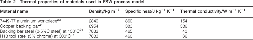
The convective heat loss from the top surface of aluminium workpiece was 10 W m−2 K−1,22 and the convective heat loss from the bottom of the steel backing bars was 1000 W m−2 K−1, which was used by Colegrove et al. 5 The thermal material properties of the materials used in the model are shown in Table 2.
Thermal properties of materials used in FSW process model
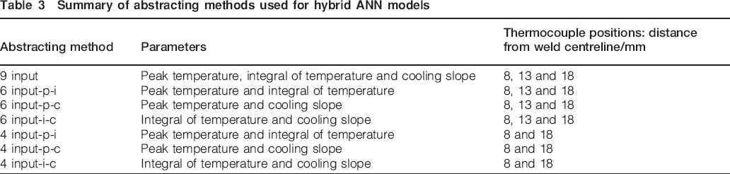
Summary of abstracting methods used for hybrid ANN models
Describing the material flow behaviour is one of the most essential parts for modelling the FSW process. This work used a modified version of Zener–Holloman law proposed by Sellars and Tegart,14 which is widely used for aluminium alloys.15, 16 Figure 2 shows the modified constitutive behaviour used in this work, which includes softening as the temperature approaches the solidus.
Artificial neural network model development
As described in the section on ‘Structure of hybrid model’, the aim of the ANN is to find the values of the CSRR and contact gap conductance parameters a and b. Travel speed was not included because it was known from the welding experiment. One of the key requirements of the hybrid model was abstracting the thermal curves before inputting them into the ANN. Several abstracting methods were investigated and are shown in Fig. 3 and are summarised in Table 2.
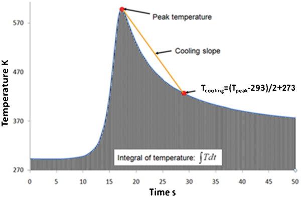
Methods for abstracting thermal profile
The three methods are the peak temperature, cooling slope and integral of temperature. The cooling slope is the slope of the line between the peak temperature and the temperature at half this value. When calculating the integral, the time over which the temperature was integrated varied for the different travel speeds and equalled the length of plate divided by the travel speed. The three methods were applied at distances of 8, 13 and 18 mm from the weld centreline, which correspond to the location of the thermocouples.
The fundamental components of the ANN model are the ANN topology, transfer function and training algorithms.25 The overall applied transfer function was the sigmoid equation. The back propagation algorithm was used throughout the study with the Levenberg–Marquardt gradient decent method. Three ANN topologies were investigated in this study:
the multilayer perceptrons network with three hidden layers: nine in the first, six in the second and third in the third.
the generalised feedforward network (GFF) with three hidden layers: nine in the first, six in the second and three in the third.
the modular feedforward network with three hidden layers: five in the first, five in the second and five in the third.
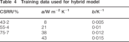
To train the hybrid model, three CSRR values and four values of the backing bar constants a and b were used, giving 48 combinations at each travel speed. The applied values are shown in Table 4.
Training data used for hybrid model
To compare the predicted thermal profiles with the experimental curves, the mean relative error (MRE) was found using
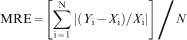
Results and discussion
Topology and abstraction method investigation
The average prediction qualities were calculated by averaging across the six travel speeds for each abstracting method and ANN topology and are shown in Fig. 4, with the error bars indicating the 95% confidence interval of the mean. Overall, the difference in MRE values for the different abstracting methods is relatively small, particularly when taking into account the variance in the mean, which is also shown in Fig. 4. Nevertheless, the 4 input-i-c method, which used the integral of temperature versus time and the cooling slope, had consistently lower MRE for the three ANN topologies. The lowest overall MRE was obtained when the GFF topology was used with this abstracting method. Table 5 shows the individual MRE values at the different travel speeds for this abstracting method and indicates that the MRE was greatest for the 4 mm s−1 travel speed.
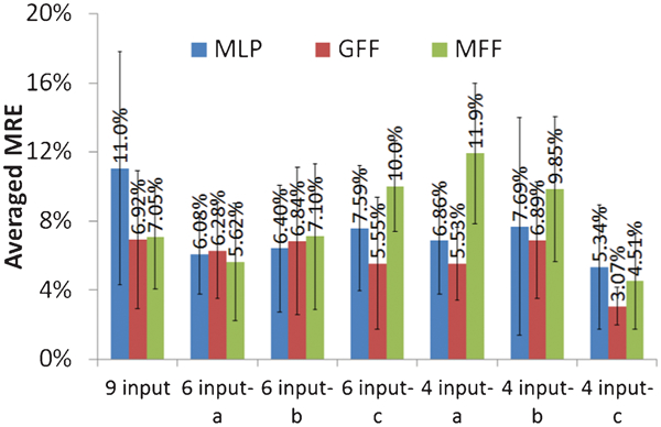
Average MRE for different abstracting methods and ANN topologies including 95% confidence interval of mean (note that different abstracting methods are defined in Table 3)
Mean relative error for 4 input-i-c abstracting method with GFF topology for different travel speeds

Hence, the additional information provided by the 6 and 9 input methods, which include the peak temperature at more locations, did not lead to any improvement in the overall prediction quality. Any changes in the overall temperature were captured adequately by the integral of temperature against time with the 4 input-i-c method. Of the three ANN topologies, the GFF method provided the best predictions.
A visual comparison between the experimental measurements and those from the 4 input-i-c method is shown in Fig. 5. The comparison shows that all the predicted curves were able to give good predictions of the thermal cycles, particularly the peak temperature. In most cases, the hybrid models were able to give accurate predictions of the cooling slopes.
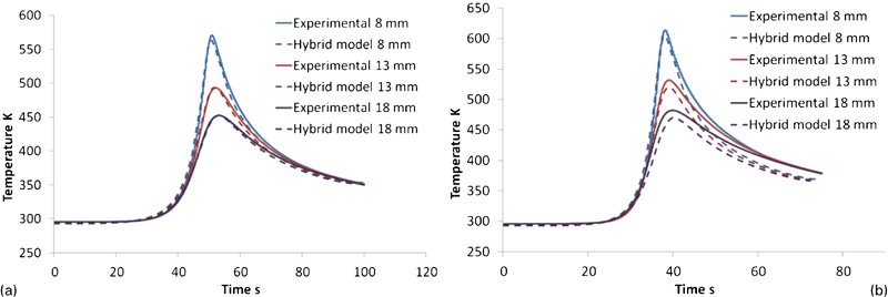
Comparison between thermal profiles predicted from hybrid model that used 4 input-i-c abstracting method with GFF topology and experimental thermal profiles for travel speeds of best fitting one (a 3 mm s−1) and worst (b 4 mm s−1)
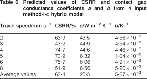
The predicted CSRR and boundary conditions for the different travel speeds are shown in Table 6 for this abstracting method and topology. The predicted values of the contact gap conductance parameters a and b from Table 6 were used to plot the contact gap conductance as a function of temperature in Fig. 6. The visual comparisons and the predicted values in Table 6 suggest that the thermal boundary condition performance and the CSRR are not independent of each other. For instance, the 5 mm s−1 case had a larger contact gap conductance, while the CSRR value is also higher at 70·9%. Hence, the larger CSRR, which resulted in more heat being generated, is balanced by a higher contact gap conductance, which increased the heat loss. The situation is also complicated by variations in the welding process. These issues are investigated in greater depth in the next section.
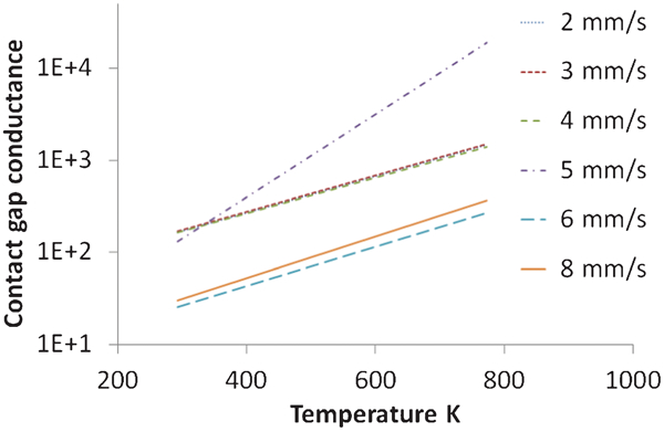
Contact gap conductance versus temperature from predicted contact gap conductance coefficients a and b in Table 6
Predicted values of CSRR and contact gap conductance coefficients a and b from 4 input method-i-c hybrid model
Investigation into variable fitting constants
Colegrove et al. 5 showed that it was possible to find a universal set of fitting constants that suit all welding parameters. The previous section found that the fitting constants depended on the travel speed. Therefore, the average values from Table 5 were applied to each of the welds, and the quality of the fit was determined.
The cooling slope was predicted well in all cases. However, there were some discrepancies in the peak temperature, which are summarised in Fig. 7. The predictions for the 2, 5 and 8 mm s−1 welds were reasonably good, with the difference in the peak temperature being <16 K. The 4 and 6 mm s−1 models have largely underpredicted the experimental results, while the 3 mm s−1 model largely overpredicted them.
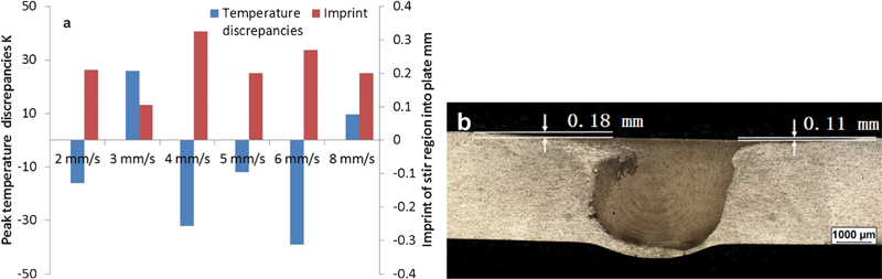
a discrepancies in peak temperature (positive for overprediction and negative for underprediction) between experimental and predicted thermal curves with averaged fitting coefficients, and measured imprint of stir region into plate and b measurement of imprint of FSW tool into workpiece material (this particular macro is from 3 mm s−1 travel speed weld where there was less penetration)
One of the reasons for variability in thermal measurements between nominally identical welding conditions is the plunge depth or the plunge force (depending on whether the FSW machine works in force or displacement control). Tang et al. 26 showed that the temperature increases with plunge depth. The Flexi-Stir machine used displacement control, and different values were used for the different welding conditions. To understand the variation in displacement between the welds, the imprint of each weld into the plate was measured as shown in Fig. 7b. Note that considerable deformation occurred under the weld due to the copper backing bar used for Flexi-stir machine (see Fig. 1). The imprints were measured on both sides of the weld stir region, and the values were averaged. These values are summarised in Fig. 7a.
The results showed that where there was a good temperature prediction, (2, 5 and 8 mm s−1), the imprint depth was ∼0·20±0·01 mm. For the 3 mm s−1 weld, the temperature was overpredicted by the model and the imprint was only 0·105 mm. This indicates that during the welding process, the tool position was higher compared to those with an imprint of 0·2 mm. Hence, the contact between the shoulder and the material was poorer, leading to less heat generation. This was also reflected in a lack of coalescence defect for this weld, which is shown in Fig. 7b. The poorer prediction may also be due to a poor contact between the workpiece and the copper backing bar from the plate lifting reflected by the large bulge on the bottom of the workpiece. For the 4 and 6 mm s−1 welds, the temperature values were underpredicted by the model. The imprint depths were 0·325 and 0·27 mm for these welds, indicating that the tool plunged further into the material. This leads to better contact with the material and greater heat generation, so the model underpredicted the temperature. Therefore, the discrepancies between the model that used averaged input parameters and the experiments may be due to the variability in the plunge depth used during the welding experiments.
Conclusions
A hybrid model of FSW was developed by combining a process model with an ANN model. The technique was used to investigate the thermal boundary conditions at the interface between the workpiece and backing bar, as well as the CSRR. The following were demonstrated.
The hybrid model was able to predict suitable values for the temperature dependent thermal boundary condition parameters and the CSRR.
A GFF topology for the ANN with four abstracted inputs based on the integrated temperature versus time and the cooling slope gave the best prediction of the experimental temperature.
The analysis indicated that the CSRR and the thermal boundary conditions were not independent of each other. Hence, a high CSRR could be offset by a high heat loss to the backing bar.
Although the initial analysis indicated that it was not possible to find a universal set of fitting parameters for these welds, further analysis indicated that when average values were applied across the welds, good predictions of the weld thermal cycles were obtained across the travel speeds. The variability that was observed could be attributed to the variation in the plunge depth, which was reflected in the weld imprints.
Footnotes
Acknowledgements
The authors would like to acknowledge the support from the Virtual Institute for Improving Performance and Productivity of Integral Structures through Fundamental Understanding of Metallurgical Reactions in Metallic Joints (VI-IPSUS). The VI-IPSUS is an initiative of the Helmholtz Association coordinated by the Helmholtz-Zentrum Geesthacht.