Estimation of current path area during small scale resistance spot welding of bulk metallic glass to stainless steel

Abstract

The current path area is a significant factor in estimating the temperature distribution via numerical modelling for resistance spot welding. This paper presents a method for the estimation of the current path area at the faying surface during small scale resistance spot welding between bulk metallic glass and stainless steel. Observation of cross-sections and fracture surfaces reveals the welding process at the faying surface for both dissimilar and similar welding. The equipotential surface that depends on the difference between the contact area of the electrode-to-sheet and sheet-to-sheet interfaces is estimated by numerical modelling. The current path area at the faying surface is estimated by measuring the electric potential between the sheets, taking into account the current distribution.

Keywords

Current path area Dynamic resistance Resistance spot welding Equipotential surface Fringing field Microjoining

Introduction

Bulk metallic glasses (BMGs) are candidates for use as widely functional materials because of their unique properties, such as a low Young's modulus and high strength. In order to take advantage of their unique properties, they need to be welded to other conventional structural alloys, such as stainless steels. However, it is well known that most amorphous alloys are embrittled by the application of heat, which leads to structural relaxation, phase separation, and crystallisation. Fast heating and cooling rates are necessary for the successful welding of BMGs.

BMGs were recently reported to be successfully welded without crystallisation via fusion processes, such as electron beam welding,1, 2 laser welding,3, 4 and resistance spot welding (RSW).5 Among them, RSW is the only process that does not require a controlled atmosphere, because the molten metal is never exposed to the atmosphere. This is a significant advantage, particularly for the fusion welding of Zr based BMGs, because they are sensitive to oxidisation. Although RSW is a suitable fusion process for similar welding of BMGs, there are issues that need to be resolved before the application of RSW to dissimilar welding of BMGs. The formation of brittle intermetallic compounds (IMCs) when two different metals are welded is unfavourable. In dissimilar welding of a Zr based BMG to stainless steel via small scale resistance welding, the stainless steel can melt, forming a brittle IMC weld nugget at the weld interface, which degrades the joint quality.6 Therefore, controlling the distribution and hysteresis of the temperature is vital in order to avoid either the crystallisation of BMGs or the formation of brittle IMCs at the RSW interface. However, it is impossible to measure the temperature in the weld directly using a thermocouple because a high current, on the order of several hundreds of amperes in small scale RSW, flows between sheets. Moreover, when at a small scale, the weld zone is too small to place a thermocouple in. Harlin et al.7 reported that the approximate distribution of temperature in RSW steels could be estimated by microstructural observation. However, the weld nugget of BMGs is invisible because no significant microstructural change is observed in both the weld and the heat affected zone (HAZ) if no crystallisation occurs.5 Therefore, it is difficult to approximate the temperature distribution via microstructural observation in the case of RSW of BMGs. Cho et al.8 observed nugget formation in a 1·4 mm thick steel directly by using half-section-truncated dome-type electrodes and a high speed camera. However, the phenomenon observed by using half-section electrodes is different from what is observed by using regular electrodes. Moreover, as described above, it is difficult to directly observe the molten nugget in small scale welding owing to its small size. Therefore, numerical simulations, such as finite element method (FEM) analysis, are often applied to calculate the temperature distribution and hysteresis in RSW. Wei et al. 9 precisely calculated the temperature hysteresis and distribution, accounting for the electromagnetic force, heat generation at the electrode-to-sheet and sheet-to-sheet interfaces, and dynamic electric resistance. The model carefully considered the contact and bulk resistances. However, for the simulation of the RSW process through analytical models, both the current path area and the contact resistance should be estimated carefully because the heat generation is proportional to the forth power of the current path area. Khan et al.10 estimated the contact area at the faying surface by the stress distribution, taking into account the plastic deformation of the workpiece and the electrode. In some cases, the contact area is assumed to be the same as the current path area.8 However, the current path area is not always equal to the contact area. Nakata et al. 11 estimated the current path area by measuring the electric potential between the electrodes for the RSW of steels. Similarly, many studies have been reported on the modelling of conventional large scale RSW.10,12^– 14 However, only a few studies have addressed the FEM analysis of small scale RSW.15 Moreover, the physical properties of BMGs are vastly different from those of conventional alloys. Table 1 lists several physical properties of a Zr based BMG and stainless steel. The electric resistivity of the Zr based BMG is three times that of the stainless steel, and the thermal conductivity is smaller than that of stainless steel. In addition, the BMGs have a wide supercooled liquid region between the solid and liquid phases. Because the supercooled liquid has a high viscosity, the simulation must include the potential for large deformation. As just described, prior research lacks essential data to estimate the temperature distribution, such as the current path area, contact resistance, and material properties at elevated temperatures.

Table 1

Physical properties of Zr₅₀Cu₃₀Ni₁₀Al₁₀ alloy and stainless steel

	Zr₅₀Cu₃₀Ni₁₀Al₁₀	SUS304
Electric resistivity (293 K)/10⁻⁸ Ω m	205	72
Electric resistivity (at melting point T_m)/10⁻⁸ Ω m	164	140
Thermal conductivity/W m⁻¹ K⁻¹	∼10	16·3–25·1
Melting point T_m/K	1133*	1673–1723
Glass transition temperature/K	706*	…

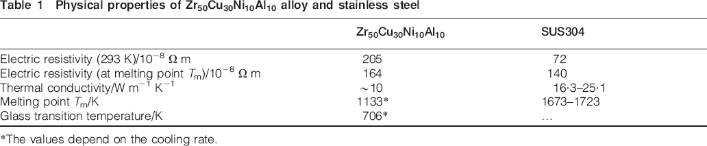
*The values depend on the cooling rate.

In the present study, small scale RSW was carried out between a BMG and stainless steel. The cross-sections of the joints and the fracture surfaces were observed. The main objective of this work was to estimate the current path area, which is a significant factor for heat generation, at the weld interface by measuring the electric potential between the sheets and accounting for the current distribution.

Experimental procedures

The materials used in this study are a Zr₅₀Cu₃₀Ni₁₀Al₁₀ BMG alloy and austenitic stainless steel (SUS304) that were 200 μm thick. The BMGs were prepared via ladle arc melt squeeze casting. The ingot material was ground to 200 μm thickness, and a sample piece approximately 25 mm in length and 5 mm in width was cut from it. The surface of the BMG sheets was polished using a no. 4000 emery paper, and the stainless steel sheets were used as received. They were cleaned with acetone before welding. The welding process was performed with a Miyachi MDB-2000B transistor type DC power supply and a Miyachi MH-D20A weld head. Cu–Cr electrodes with a diameter of 3 mm and a round tip surface with a curvature of 3·8 mm were used. Small scale RSW was carried out with a welding current of 500 A and a weld time of 1–9 ms. The electrode force was 49 N. The experimental setup is shown in Fig. 1. The dynamic signals were monitored using a data acquisition system. The voltage U₀ measured by the current sensor was converted to the welding current I. The electric potential drop across the sheet-to-sheet interface was recorded as U₁ with a sampling rate of 25 kHz. The dynamic resistance through the interface was represented by U₁/I. An end terminal was placed at the end of each sheet (Fig. 1b).

Figure 1

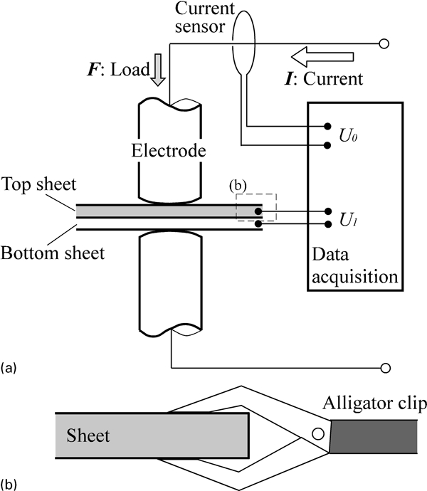
Experimental set-up of resistance spot welding

The as welded joints were fractured by peel tests and the fractured surfaces were observed by scanning electron microscopy (SEM). The cross-sections of the joints were also observed by SEM after electrochemical etching with oxalic acid. The footprint of the electrode on the sheet surface was observed by a laser microscope. In order to measure the distribution of the pressure at the sheet-to-sheet interface, that is, the faying surface, three types of pressure sensitive papers were used. The pressure measurement ranges of the papers were 2·5–10, 10–50 and 50–130 MPa.

An axisymmetric electrical model for RSW was solved by ANSYS to predict the map of the equipotential surface for a sheet (Fig. 2). This model simulates the current flow from the top of the electrode-to-sheet interface to the faying surface of the top sheet. The parameters r_es and r correspond to the radii of the current path area at the electrode-to-sheet and sheet-to-sheet interfaces respectively. The current flows from the area of a circle with radius r_es to the area of a circle with radius r. A rectangular current distribution of 500 A was provided to the current path area at the electrode-to-sheet surface. The electric potential of the current path area at the sheet-to-sheet interface was set to zero. The mesh size was 10×10 μm. The current distribution after 1×10⁻⁵ s of current flow was calculated. The following major assumptions were incorporated:

Figure 2

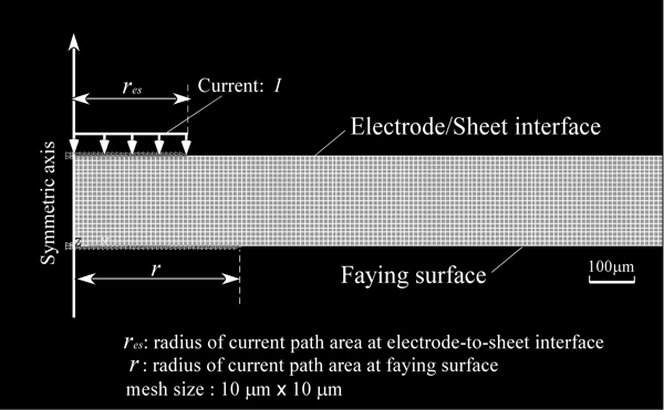
Finite element model to calculate distribution of current and equipotential surface

the temperature distribution in the sheet does not affect the current distribution

the physical properties shown in Table 1 at room temperature were used

iii

the deformation of the sheet is negligible

the current distribution at the electrode-to-sheet interface is uniform.

Results

Cross-sections

The results of the metallurgical examination of weld cross-sections for similar and dissimilar joints are shown in Fig. 3. In the case of the similar welding of SUS304, a weld nugget and a HAZ formed quickly at a weld time of 2 ms. The weld nugget and HAZ grew with increasing weld time. Alternatively, when the stainless steel was welded to the BMG sheet, no weld nugget was observed at a weld time of 2 ms. Squeezed out metallic glass was observed at the end of the weld interface, which is shown by the arrows in Fig. 3a. The formation of the squeezed-out BMG suggests that a liquid phase of BMG could have existed near the weld interface, even at a weld time of 2 ms. No significant weld zone was formed in the stainless sheet with a dissimilar joint at a weld time of 2 ms, despite the weld nugget formation for the similar welding of stainless sheets at the same weld time, as shown in Fig. 3d. When a weld was formed without an IMC nugget, as in Fig. 3a, only a limited fusion of stainless steel occurred at the centre of the weld interface to form a weld.15 For the RSW, the heat generated can be expressed as (1) where Q is the heat generation, I is the current, R is the resistance (including contact and bulk), and t is the weld time. The resistivity of the BMG is much larger than that of the stainless steel. As long as the current path area in dissimilar welding is equal to that in similar welding, the resistance heat in dissimilar welding must be larger than of similar welding. A rapid increase in the current path area due to the liquefaction of the BMG decreased the resistance during dissimilar welding, which caused no fusion in the stainless steel sheet at a weld time of 2 ms. The stainless steel began to melt at a weld time of 4 ms, resulting in the formation of an IMC nugget owing to the mixture of both molten metals. The IMC nugget grew with increasing weld time.

Figure 3

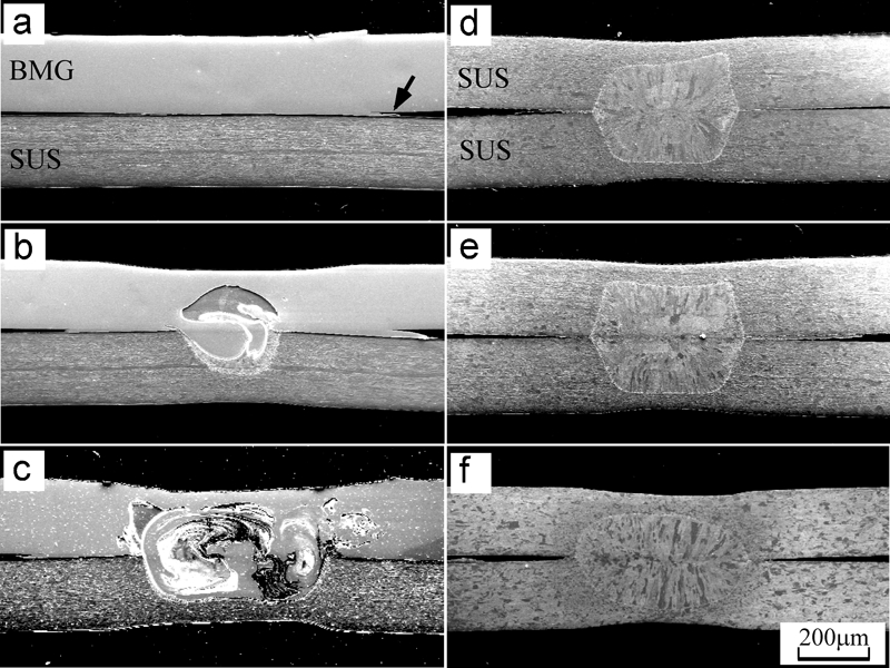
Cross-sections of a–c dissimilar and d–f similar joints made with different weld times, from 2 to 9 ms, at welding current of 500 A: arrow shows squeezed-out metallic glass

Fractured surfaces

Fractured surfaces of a BMG in a dissimilar joint and stainless steel in a similar joint are shown in Figs. 4 and 5 respectively. The squeezed-out BMG shown in Fig. 3a was observed in the outermost region of the dissimilar welding. Two types of regions, in addition to the squeezed-out BMG, were observed on the fracture surface of the BMG. For the squeezed-out BMG, a region with many straight lines in one direction was observed. These line patterns were transferred from the surface of the stainless steel, but no Cr or Fe was detected there. The stainless steel in a solid state did not react, but when it contacted the BMG in a liquid or supercooled liquid state, it did react in a region, which is termed region I. Inside region I, there was a bright region that contained a small amount of Fe and Cr from the stainless steel, which is termed region II. Region II is where the liquid of the BMG reacts with the stainless steel in a solid state.16 With increasing weld time, the temperature rises above the melting point of stainless steel, which leads to the formation of an IMC nugget. In contrast, in the similar welding of stainless steel, there were two regions: a weld nugget and an HAZ on the fracture surfaces. The HAZ was visible around the weld nugget.

Figure 4

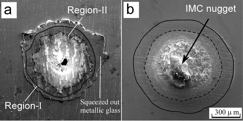
Fractured surfaces of BMG of dissimilar joints made with different weld times of a 2 ms and b 9 ms: solid and broken lines show region I and region II respectively.

Figure 5

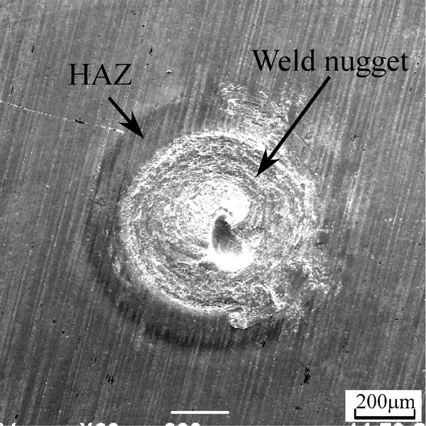
Typical fractured surface of SUS304 similar joint made with weld time of 9 ms

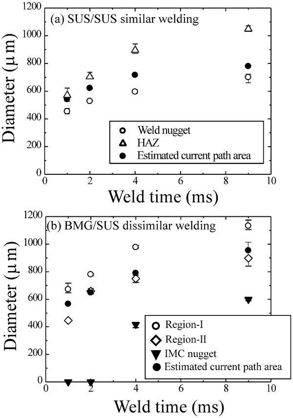
The changes in each region with respect to the weld time area are shown in Fig. 6. Also plotted in Fig. 6 are the areas of the footprint of the electrode on the sheets. For similar welding, the weld nugget grew gradually with increasing weld time, and the weld nugget size was nearly saturated at a weld time of 9 ms because of the competition between thermal conductivity and heat generation. For dissimilar welding, region I and region II also grew with increasing weld time, but the growth rate of the region II for the first 2 ms was slightly larger than that of the weld nugget for similar welding.

Figure 6

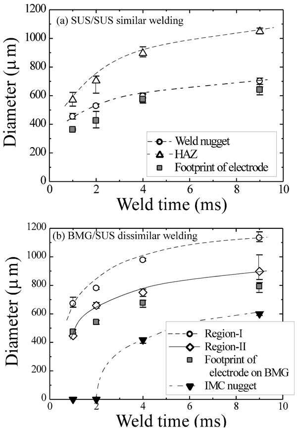
Change in each region as function of weld time: a SUS/SUS similar welding and b BMG/SUS dissimilar welding

Dynamic resistance

The mechanism of RSW is known to be based on Joule heat, which can be mathematically described by equation (1). The resistance includes a contact resistance at the electrode-to-sheet and sheet-to-sheet interfaces, and a bulk resistance of the base materials. Much research on the dynamic resistance measurements of large scale RSW has been reported because the dynamic resistance curve is suggested to be suitable for quality control. Dickson et al. 17 summarised the theoretical dynamic resistance curves of the large scale RSW of steels, and proposed six stages to characterise the dynamic resistance based on the competition between the bulk and contact resistances. At the beginning of the welding, the sheet-to-sheet resistance experiences a very sharp drop because of the oxide film or contamination breakdown. Subsequently, asperity softening causes the resistance to decrease further. However, the increasing temperature results in an increase in the bulk resistivity. With increasing temperature, the change in the dynamic resistance depends on phenomena such as melting, nugget growth, and increase in the contact area for current flow and expulsion. Tan et al. 18 reported the detailed dynamic resistance curve for the small scale RSW of nickel sheets. However, compared to the research on large scale RSW, limited research has been conducted on the dynamic resistance in microscale or small scale RSW.

Figure 7 shows the sheet-to-sheet dynamic resistance at a welding current of 500 A for similar and dissimilar welding. Although the dynamic resistance decreased during the current carrying in both cases, some differences were observed between similar and dissimilar welding, especially in the early stage. For similar welding, the resistance first increased and then decreased after reaching a peak value. It continuously decreased until 2 ms passed, and then, it remained approximately constant. As Wen et al. 18 reported, the first increase in the resistance was probably caused by asperity heating. The decrease after the peak may have been due to the asperity softening and an increase in the real contact area. In the same stage, a weld nugget also formed (see Fig. 3d), although an obvious increase in the resistance was not detected. For dissimilar welding, the initial increase in resistance due to asperity heating was not observed. The resistance then sharply dropped for 0·2 ms and continuously decreased until 2 ms. Because the resistivity of the BMG is three times that of stainless steel (see Table 1), the temperature increases drastically once the current flows. This caused the BMG to melt in a short amount of time, rapidly increasing the contact area, which caused the drastic drop in resistance at the beginning of the welding. The rate of decrease in resistance is smaller than that during the first drastic drop because of the temperature increase. The small peak observed at 2 ms was possibly caused by the melting of the stainless steel. The resistance gradually decreased with increasing weld time because of the increase in the current path area after 2 ms.

Figure 7

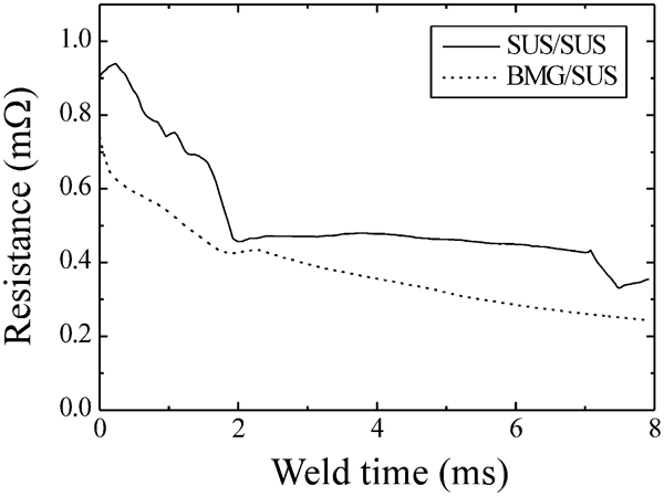
Dynamic resistance curves for similar and dissimilar welding at 500 A

Electric potential in measurement

The sheet-to-sheet resistance R includes the bulk resistance as well as the contact resistance at the faying surface. The bulk resistance R_B is calculated using the following equation (2) where ρ is the resistivity, L is the length of the current path and A is the area of the current path.18 In the present study, the sheet-to-sheet electric potential drop U₁ was measured at the ends of both the top and bottom sheets, as shown in Fig. 1; this is the general method for measuring electric resistance in RSW. Figure 8 shows a schematic illustration of the welding setup, including the current path, equipotential lines, and measurement points. The equipotential lines are determined according to the current path. The current flows in a curved path in the sheet near the edge of the electrode, which forms a fringing field. As a result, the equipotential map depends on the current distribution at the edge of the electrode. As shown in Fig. 8, both the top and the bottom surfaces of the sheet have the same electric potential at the end of the sheet, as long as the measurement point is at a sufficient distance from the current path area. The potential drop measured at the end of the sheets corresponds to a part of the sheets, which is denoted as 2l in Fig. 8. Therefore, the net length of the current path of 2l is used in equation (2) instead of L. The distribution of the current depends on the difference between the diameters of the electrode-to-sheet contact area (2r_es) and the sheet-to-sheet contact area (2r). The difference is hereafter described as ΔD ( = 2r−2r_es). The distribution of the current path as a function of ΔD was calculated via finite element analysis. Figure 9 shows results of an FEM analysis of the dependence of the equipotential surface maps on ΔD. Additionally, the net length of the current path in a sheet l changes with ΔD. Figure 10 shows the relationship between ΔD and the net length of the current path l in a sheet. The net length of the current path decreases with increasing ΔD. The regression formula is expressed as follows (3)

Figure 8

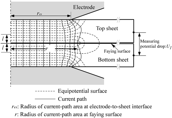
Schematic illustration of relationship between equipotential lines and current path during RSW: value of 2l corresponds to net length of current path, which contributes to electric potential drop U₁ between sheets

Figure 9

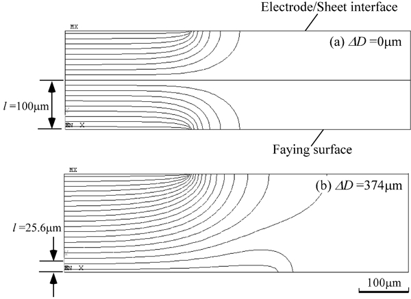
Effect of current path area on equipotential surface: difference of current path area between sheet-to-sheet (faying surface) and electrode-to-sheet interfaces (ΔD) affects measured potential; equipotential lines are drawn at every 5% of total potential from electrode-to-sheet interface to faying surface

Figure 10

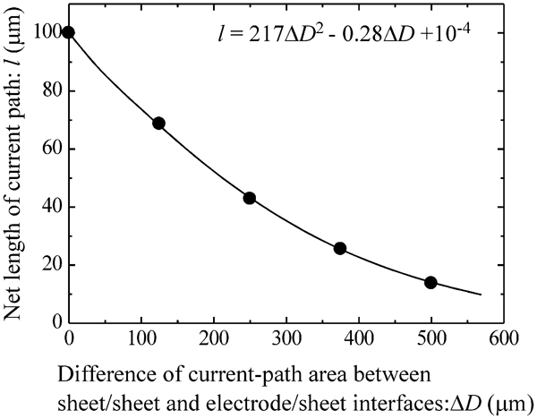
Relationship between current path length l and difference of current path area between electrode-to-sheet and sheet-to-sheet interfaces ΔD

Discussion

Estimation of current path area

The initial pressure distribution at the faying surface under electrode force without current was measured with pressure sensitive papers (Fig. 11). The pressure decreased from the centre to the periphery in both the similar and the dissimilar sheet combinations. This suggests that the static contact resistance at the faying surface differs from the centre to the periphery. The contribution of the contact resistance to the heat generation is significant for RSW, especially for smaller scales. However, it is difficult to estimate the contact resistance through the stress distribution. It is assumed that the contact resistance vanishes immediately once the current begins flowing in the case of dissimilar welding. In fact, the dynamic resistance dropped sharply at the beginning of the welding owing to the rapid increase in contact area (see Figs. 3a and 7). After a weld time of 1 ms, the contact resistance is negligible.

Figure 11

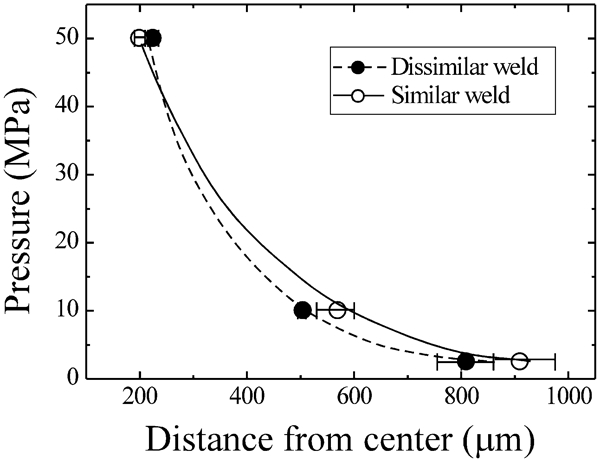
Initial pressure distribution at faying surface

In order to estimate the current path area at the faying surface, two types of models were used in which current flows were considered for dissimilar welding. Figure 12 shows the models of the current path that contributes to the measurement of electric potential. As shown in Fig. 3b, the stainless steel begins to melt after a weld time of 4 ms for dissimilar welding. In model 1, the liquid BMG is welded to solid stainless steel for 2 ms. In model 2, the liquid BMG, molten nugget, and solid stainless steel coexist after a weld time of 4 ms. The weld zone included both materials. Since the resistivity of the molten IMC nugget was not known, the resistivity of molten stainless steel was adopted in place of the molten nugget in model-2. Since this is an axisymmetric model, the measured resistance corresponds to the resistance of the cylinder that composes several phases; it has a diameter of 2r and a height of 2l. Model-1 is composed of only serial resistances and model-2 is a combination of serial and parallel resistances. Similar welding of stainless steel corresponds to model 2, except that there are only two phases, SUS(S) and SUS(L). The resistance of the models can be determined by the following parameters: l, r, and r₀, and the resistivity of each phase. r₀ is the radius of the molten nugget. The measured electric potential drop U₁ is expressed as (4) The relation among R_B, ΔD, and l is shown with equations (2) and (3).

Figure 12

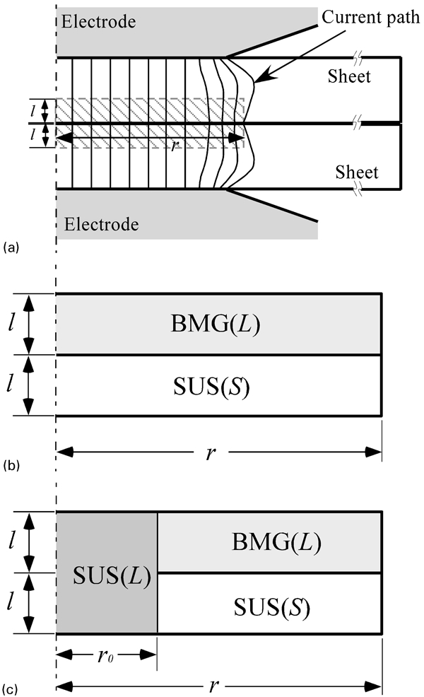
Models of measurement region b before and c after formation of molten nugget: images b and c show hatched area in a; r₀, radius of molten stainless steel; r, radius of current path area at faying surface

Therefore, the diameter of the current path area at the faying surface (2r) can be estimated by measuring the sheet-to-sheet resistance, diameter of the weld nugget, and diameter of the current path area at the electrode-to-sheet interface (2r_es). Table 1 gives the resistivity of each phase used in the presented models. The resistivity of the stainless steel just above the melting point is adopted as that of liquid stainless steel in model 2. The resistivity of the Zr₅₀Cu₃₀Ni₁₀Al₁₀ metallic glass in the liquid state has not been reported. However, the resistivity of a similar Z based metallic glass, Zr₆₀Al₁₅Ni_7·5Co_2·5Cu₁₅, has been reported; the resistivity just above the melting point is 80% of that at room temperature.19 Therefore, 80% of the resistivity of Zr₅₀Cu₃₀Ni₁₀Al₁₀ metallic glass at room temperature was adopted as the liquid state value. The diameter of the current path area at the electrode-to-sheet interface (2r_es) was measured by observing a footprint of the electrode on the sheets (Fig. 6). The change in the equipotential lines and the distribution of the current path with a varying temperature is neglected in the models. The estimated diameter of the current path area at the faying surface is shown in Fig. 13. The estimated current path area in similar welding by this method is slightly larger than a weld nugget and smaller than the HAZ. The current possibly flows in the molten region, and the HAZ is formed because of heat conduction. In the case of dissimilar welding, the estimated current path area is larger than region II and smaller than region I, corresponding more so to region II, which suggests that a reaction occurred between the liquid BMG and the stainless steel where current flowed at the faying surface.

Figure 13

Estimated current path area by dynamic resistance measurements at faying surface in comparison with various areas

After the disappearance of the contact resistance, the current path area can be estimated by monitoring the electric potential between two sheets by considering the current fringing field in the present study. Further works on the physical properties of BMGs as a function of temperature are expected.

Conclusions

The current path area at the faying surface was estimated for the dissimilar small scale RSW of bulk metallic glass to stainless steel. The major conclusions are summarised as follows.

No visible weld nugget formed in the BMG/stainless steel welding at a weld time of 2 ms because of a rapid increase in contact area. Once the stainless steel is melted, liquid metallic glass mixed with liquid stainless steel, resulting in the formation of an intermetallic compound nugget.

Dynamic resistance curves suggest that the contact resistance at the faying surface disappeared immediately at the beginning during dissimilar welding, and the current path area also increased rapidly.

The current distribution and equipotential surface varied depending on the difference between the electrode-to-sheet and sheet-to-sheet areas. They affect the net length of the current path, which contributes to the measured electric potential at the end of the sheet. The measured electric potential at the end of the sheets includes both the bulk and the contact resistances. The net volume of the bulk, which contributes to the measured potential drop, depends on the current distribution.

The current path area at the faying surface can be estimated by measuring the electric potential at the end of the sheets by considering the equipotential surfaces after the disappearance of the contact resistance. However, the temperature-dependent material properties of BMGs are necessary to estimate the current path area more accurately.

Footnotes

Acknowledgements

A part of this work was performed under the interuniversity cooperative research programme of the Institute for Materials Research, Tohoku University. Furthermore, this work was also supported by the Ministry of Education, Culture, Sports, Science and Technology of Japan via a Grant-in-Aid for Scientific Research (C), 21560750, in 2011.

References

Yokoyama

, Abe

, Fukaura

, Shinohara

, Inoue

: ‘Electron beam welding of Zr₅₀Cu₃₀Ni₁₀Al₁₀ bulk glassy alloys’, Mater. Trans., 2002, 43, 2509–2515.

Kawamura

, Ohno

: ‘Successful electron-beam welding of bulk metallic glass’, Mater. Trans., 2001, 42, 2476–2478.

Kim

, Lee

, Sun

, Shin

, Bae

: ‘Pulsed Nd:YAG laser welding Cu₅₄Ni₆Zr₂₂Ti₁₈ bulk metallic glass’, Mater. Sci. Eng. A, 2007, A449–A451, 872–875.

, Li

, Xiong

, Xing

, Wang

, Li

: ‘Laser welding of Zr₄₅Cu₄₈Al₇ bulk glassy alloy’, J. Alloys Compd, 2006, 413, 118–121.

Fujiwara

, Fukumoto

, Yokoyama

, Nishijima

, Yamamoto

: ‘Weldability of Zr₅₀Cu₃₀Al₁₀Ni₁₀ bulk glassy alloy by small-scale resistant spot welding’, Mater. Sci. Eng. A, 2008, A498, 302–307.

Fukumoto

, Minami

, Soeda

, Matsushima

, Yokoyama

, Fujimoto

: ‘Microstructural control for dissimilar joints between metallic glasses and stainless steel by resistance microwelding’, Proc. 16th Symp. on ‘Microjoining and assembly technology in electronics’, 2010, 247–250.

Harlin

, Jones

, Parker

: ‘Weld growth mechanisms during resistance spot welding of two and three thickness lap joints’, Sci. Technol. Weld. Join., 2002, 7, (1), 35–41.

Cho

, Rhee

: ‘Experimental study of nugget formation in resistance spot welding’ Weld. J., 2003, 82, (8), 195s–201s.

Wei

, Wu

: ‘Effect of electrical current on transport processes in resistance spot welding’, Sci. Technol. Weld. Join., 2010, 15, (6), 448–456.

10.

Khan

, Xu

, Chao

Y.-J

: ‘Prediction of nugget development during resistance spot welding using couple thermal-electrical-mechanical model’, Sci. Technol. Weld. Join., 1999, 4, (4), 201–207.

11.

Nakada

, Nishimura

, Otani

, Tamada

: ‘Real-time measurement of current path area of spot welds by resistance between electrode tips’, Q. J. Jpn Weld. Soc., 1984, 2, (2), 253–259.

12.

: ‘Finite element modelling of resistance spot welding of aluminium with spherical tip electrode’, Sci. Technol. Weld. Join., 2002, 7, (2), 119–124.

13.

Tsai

, Jammal

, Papritan

, Dickinson

: ‘Modeling of resistance spot weld nugget growth’, Weld. J., 1992, 71, (2), 47s–54s.

14.

Cho

, Cho

: ‘A study of the thermal behavior in resistance spot welds’, Weld. J., 1989, 68, (6), 236s–244s.

15.

Chang

, Li

, Zhou

: ‘Comparative study of small scale and ‘large scale’ resistance spot welding’, Sci. Technol. Weld. Join., 2001, 6, (5), 273–280.

16.

Fukumoto

, Minami

, Soeda

, Matsushima

, Takahashi

, Yokoyama

, Fujimoto

: ‘Microstructural development at weld interface between Zr-based glassy alloy and stainless steel by resistance microwelding’, J. Phys., Conference Series, 379, 2012, 012027.

17.

Dickinson

, Franklin

, Stanya

: ‘Characterization of spot welding behavior by dynamic electrical parameter monitoring’, Weld. J., 1980, 59, (6), 170s–176s.

18.

Tan

, Zhou

, Kerr

, Lawson

: ‘A study of dynamic resistance during small scale resistance spot welding of thin Ni sheets’, J. Phys. D: Appl. Phys., 2004, 37, 1998–2008.

19.

Kimura

, Kishida

, Kaneko

: ‘Physical and mechanical properties of Zr-based metallic glasses’, Mater. Trans. JIM, 1995, 36, (7), 890–895.