Neural network based toughness prediction in HAZ of low alloy steel produced by temper bead welding repair technology

Abstract

The pressure vessels of aged nuclear power plants are needed to repair or maintain, and temper bead welding (TBW) is one effective repair welding method instead of post weld heat treatment. For TBW, toughness is the key criteria to evaluate the tempering effect. A neural network based method for toughness prediction in heat affected zone (HAZ) of low alloy steel has been investigated to evaluate the tempering effect in TBW. On the basis of experimentally obtained database, the new toughness prediction system was constructed by using radial basis function neural network. With it, the toughness distribution in HAZ of TBW was calculated based on the thermal cycles numerically obtained by finite element method (FEM). The predicted toughness was in good accordance with the experimental results. It follows that our new prediction system is effective for estimating the tempering effect during TBW and hence enables us to assess the effectiveness of TBW before the actual repair welding.

Keywords

Toughness Neural network Temper bead welding low alloy steel FEM

Introduction

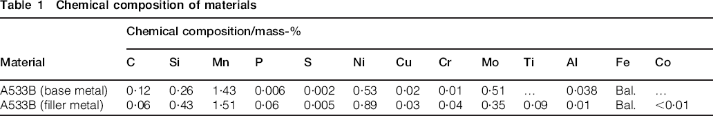
Pressure vessels are in general fabricated from steels with excellent mechanical properties. Low alloy steel ASTM A533B (equivalent to JIS SQV2A, as shown in Table 1) possessing superior low temperature toughness and weldability is widely used to build pressurised water reactor vessels in nuclear power plants. However, the excellent mechanical properties of the base metal will be altered by the thermal cycles imposed by welding processes, and the increase in hardness and the loss of toughness always occur in the heat affected zone (HAZ) of the welds.1 Serious damage may occur in some cases in the coarse grained heat affected zone (CGHAZ).2 Therefore, post-weld heat treatment (PWHT) is normally required to improve the toughness, eliminate the residual stress and decrease the hardness.

Table 1

Chemical composition of materials

Material	Chemical composition/mass-%
Material	C	Si	Mn	P	S	Ni	Cu	Cr	Mo	Ti	Al	Fe	Co
A533B (base metal)	0·12	0·26	1·43	0·006	0·002	0·53	0·02	0·01	0·51	…	0·038	Bal.	…
A533B (filler metal)	0·06	0·43	1·51	0·06	0·005	0·89	0·03	0·04	0·35	0·09	0·01	Bal.	<0·01

However, PWHT is sometimes difficult to perform in operation when repairing large scale structures. In practice, the temper bead welding technique is an effective repair welding method instead of PWHT.3, 4 Temper bead welding is a kind of multipass welding, in which the tempering effect is caused by the heat arising from the following multilayer weld thermal cycles. To achieve the required tempering effect during temper bead welding, it is very important to select the proper thermal cycle. Toughness and hardness are the key criteria to evaluate the tempering effect in temper bead welding. The toughness and hardness in the HAZ are affected by various factors such as peak temperature and cooling rate during the weld thermal cycle and the number of tempering thermal cycles. The hardness prediction systems of temper bead welding have been reported by the authors before.5 Therefore, in the present study, the toughness prediction system has been constructed using a neural network that can process the complex data involved. The proposed toughness prediction system has been verified with comparing the predicted toughness with the measured ones in the HAZ of low alloy steel A533B when temper bead welding is applied.

Temper bead welding

Four subzones of HAZ

The HAZ is that portion of the parent metal adjacent to the weld that has not been melted but whose microstructure and hence mechanical properties have been altered by the heat of welding. During welding, there can be up to four subzones within the HAZ created according to the maximum temperature reached and the duration of time at that temperature. As illustrated in Fig. 1, these four subzones are: coarse grained HAZ (CGHAZ), fine grained HAZ (FGHAZ), intercritical HAZ (ICHAZ) and subcritical HAZ (SCHAZ). Among these, CGHAZ always has poor mechanical properties due to the increase in hardness and loss of toughness.1, 2, 6 Therefore, tempering is required to improve the mechanical properties.

Figure 1

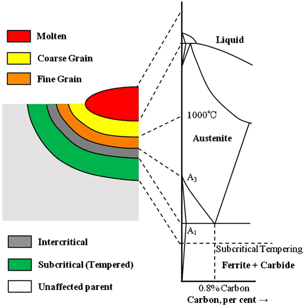
Iron carbon phase diagram showing transition points relating to weld HAZ

Definition and technique of temper bead welding

The ASME Boiler and Pressure Vessel code defines temper bead welding as follows: ‘A weld bead placed at a specific location in or at the surface of a weld for the purpose of affecting the metallurgical properties of the heat affected zone or previously deposited weld metal’. It has applications in the pressure equipment industry for repairs and modifications.

Five temper bead welding techniques have been developed over the past 20 years: (a) half bead technique; (b) consistent layer technique; (c) alternate temper bead technique; (d) controlled deposition technique; and (e) weld toe tempering technique.7 All techniques are similar in the goal of tempering the CGHAZ in the parent metal.

In the present study, consistent layer technique is mainly considered, because this technique is theoretically most orthodox one.

Thermal cycle analysis of consistent layer technique

For the one-layer welding, as shown in Fig. 2, there are two kinds of thermal cycles occurred in HAZ of temper bead welding: single cycle (one-cycle) (Fig. 2b), which is effected by one-pass welding; double cycles (two-cycle) (Fig. 2b), in the middle overlapped region of two-pass welding.

Figure 2

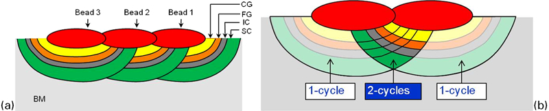
Schematic illustration of one-layer welding

Figure 3 presents a schematic illustration of multilayer welding produced by the consistent layer technique.7 In this technique, the HAZ of the first layer is only tempered but has not retransformed by the subsequent layers, because this technique places the Ac₁ retransformation line of the second layer welding within the fusion zone produced by the first layer welding, as shown in Fig. 3b. Therefore, this technique can produce a HAZ microstructure that consists predominantly of tempered martensite with small amounts of bainite, resulting in good toughness properties. Because there are only tempering thermal cycles from the second layer welding in consistent layer technique, the possible thermal cycles after multilayer welding are one-cycle+temper and two-cycle+temper.

Figure 3

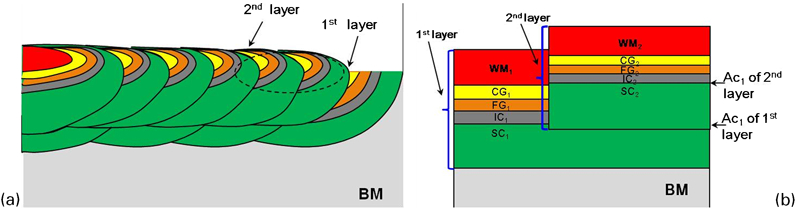
Schematic illustration of temper bead welding produced by consistent layer technique

Therefore, as shown in Fig. 4, the thermal cycles in the HAZ of temper bead welding produced by the consistent layer technique are most simply classified as the following four types: (1) one-cycle; (2) two-cycle; (3) one-cycle+temper; (4) two-cycle+temper.

Figure 4

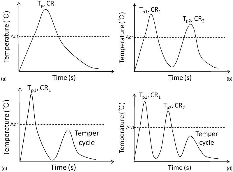
Possible thermal cycles arose in temper bead welding produced by consistent layer technique

For the one-cycle, the toughness is mainly dependent on two factors: T_p and CR.1,8^– 10 The two-cycle is more complicated, with four factors governing the toughness: T_p1 and CR₁ of the first thermal cycle, and T_p2 and CR₂ of the second thermal cycle. Here, T_pi is the peak temperature of the ith pass thermal cycle, and generally CR_i means the cooling rate from 800 to 500°C of the ith pass thermal cycle, that is, CR_i = 300/t_8,5 (°C s⁻¹). While when the T_pi of the thermal cycle is lower than 800°C, the cooling rate from T_pi to 400°C is taken as CR_i, CR_i = (T_pi−400)/Δt (°C s⁻¹). Besides these factors, the temper parameter is also included in the one-cycle+temper and two-cycle+temper. And the tempering effect of all the temper thermal cycles can be considered to be expressed as a factor, thermal cycle tempering parameter (TCTP), proposed by the authors, by extending the Larson–Miller parameter (LMP) to non-isothermal heat treatment.5

To apply LMP to temper thermal cycle process, the thermal cycle was divided into small increments where each increment could be regarded as an isothermal heat treatment with a ‘short’ holding time. The overall tempering effect during the thermal cycle process is considered as the sum of the ‘short’ isothermal heat treatments.

The temper parameter of the first segment at T₁ with holding time t₁ is equal to that at T₂ with equivalent holding time t_1,2, shown as (1) Thus, the temper parameter of the combined first and second segments can be expressed as (2) Similarly, the overall temper parameter from the first segment to third segment can be obtained as (3) In turn, the temper parameter of the whole thermal cycle, from the first segment to the n^th segment (the last segment), can be expressed as (4) where T_n is the temperature of the n^th segment, t_n is the holding time of the n^th segment and t_n−1,n is the equivalent holding time from the first to the (n−1)^th segment at the temperature of T_n. T_n is calculated as (T_i+T_i+1)/2. T_i and T_i+1 are the temperature of the start point and the end point of the segment respectively.

The proposed TCTP has been proved can be applied to evaluate quantitatively the tempering effect and the hardness change during both thermal cycle tempering processes and multipass isothermal heat treatment.5 In a word, the mechanical properties (hardness, toughness, etc.) after all kinds of thermal cycles are determined by the following five parameters: T_p1, CR₁, T_p2, CR₂ and TCTP.

Materials and experimental procedures

The chemical compositions of the base metal, low alloy steel A533B, and filler material A533B (MG-S56X) used are shown in Table 1. Samples of low alloy steel were heated by Gleeble 1500 to synthesise the as welded and temper processed HAZs. The shape and size of the sample are shown in Fig. 5a. Samples with size of Φ15×60 mm were heated by Gleeble 1500 to prepare for the Charpy impact test. In order to avoid fracture path deviation (FPD), side notched Charpy V-notch specimens were prepared from samples subjected to the simulated thermal cycles, and the size was shown in Fig. 5b. Charpy impact test was carried out at −12°C, which is the required test temperature of Charpy impact validity qualification test for TBW in nuclear power industries. The toughness was evaluated from the absorbed energy vE.

Figure 5

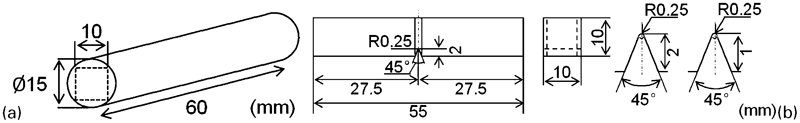
Schematic illustration of samples

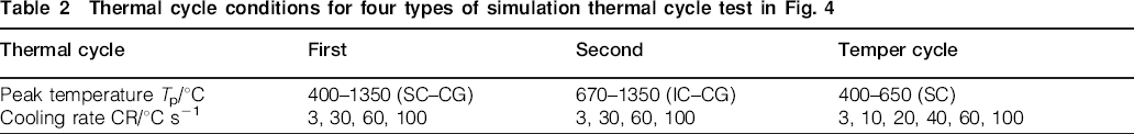
Figure 4 illustrates four types of thermal cycle patterns to simulate the thermal cycles in HAZ of temper bead welding with consistent layer technique.7 The Ac₁ and Ac₃ temperature of A533B is 670 and 837°C respectively. The thermal cycle conditions for 4 types of simulation thermal cycle test in Fig. 4 are listed in Table 2. In one-cycle, T_p1 was ranged from 400 to 1350°C, which covered the temperature range of HAZ in low alloy steel (SC–CG). In the other three types of thermal cycle, T_p1 and T_p2 were higher than Ac₁, which were used to simulate the CGHAZ, FGHAZ and ICHAZ. Therefore, T_p1 and T_p2 varied from 670 to 1350°C (IC–CG). For the tempering thermal cycle, tempering temperature is lower than Ac₁; thus, it was changed in the range of 400–650°C (SC). In all thermal cycles, CR_i covered the possible cooling rate range in HAZ of TIG welding; therefore, it varied from the lowest 3°C s⁻¹ to the highest 100°C s⁻¹.

Table 2

Thermal cycle conditions for four types of simulation thermal cycle test in Fig. 4

Thermal cycle	First	Second	Temper cycle
Peak temperature T_p/°C	400–1350 (SC–CG)	670–1350 (IC–CG)	400–650 (SC)
Cooling rate CR/°C s⁻¹	3, 30, 60, 100	3, 30, 60, 100	3, 10, 20, 40, 60, 100

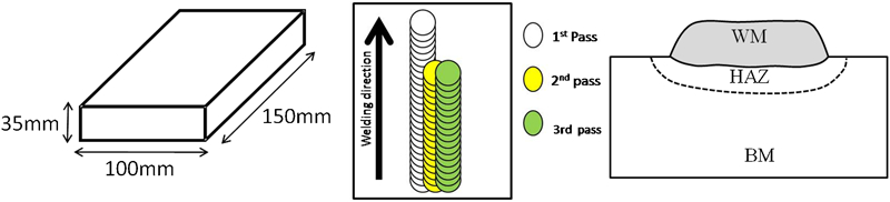
The multipass welded sample (100×35×150 mm, Fig. 6) was produced by TIG welding with the welding conditions shown in Table 3, which included seven-layer–88-pass welds. The temper bead welding was performed using consistent layer technique.7 The section surface was cut from the multipass welded sample. The side notched Charpy specimens of temper bead welding were prepared as illustrated in Fig. 7. First, the welding part was cut from the welding sample, as shown in Fig. 7a. Then, the cut part was extended by electronic beam welding (EBW) using the same material of low alloy steel A533B as presented in Fig. 7b. The distance from EBW line to bead line of TBW is farther than 4 mm to avoid the heat affect of EBW. Finally, the side notched Charpy impact samples were cut from the extended sample, as illustrated in Fig. 7c. The prepared side notched Charpy impact sample was shown in Fig. 7d, with the notch in HAZ position. Using this method, the toughness of the temper bead welded sample was evaluated from the absorbed energy vE. The thermal cycles in temper bead welding were calculated using finite element method (FEM) software developed specifically for welding simulation.11

Figure 6

Specimen of temper bead welding test

Figure 7

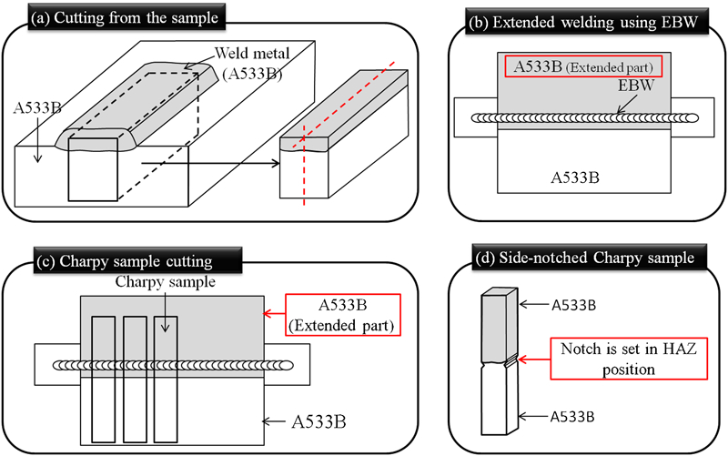
Procedure of preparing Charpy impact test specimens of TBW

Table 3

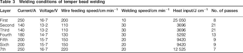
Welding conditions of temper bead welding

Layer	Current/A	Voltage/V	Wire feeding speed/cm min⁻¹	Welding speed/cm min⁻¹	Heat input/J cm⁻¹	No. of passes
First	250	16·7	200	10	25 050	8
Second	140	13·2	110	30	3696	21
Third	140	13·2	110	30	3696	21
Fourth	180	14·7	130	30	5292	13
Fifth	200	15·7	150	20	9420	9
Sixth	200	15·7	150	20	9420	9
7th	250	16·7	220	20	12 525	7

Experimentally measured toughness database

It is very important to have a correct evaluation of toughness in HAZ. However, due to the HAZ narrowness and microstructural and mechanical gradients, FPD phenomenon often occurred in standard Charpy testing,12 as shown in Fig. 8a. In order to avoid FPD, the absorbed energy of side notched Charpy impact samples was used as the database. The relationship between absorbed energy of side nothed Charpy V-notch samples (vE_SN) and standard Charpy V-notch samples (vE_STD) are shown in Fig. 8 b, which can be expressed as follows (5) The toughness database used in the present study is the absorbed energy of side notched Charpy impact samples.

Figure 8

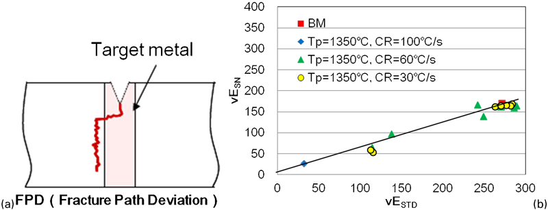
Comparison of standard and side notched absorbed energy

Toughness database of one-cycle

Figure 9 shows the relationship between the absorbed energy of the side notched Charpy impact test and the peak temperature of one-cycle for four cooling rates (3–100°C s⁻¹). The perk temperature has great influence on the absorbed energy after one-cycle, and the absorbed energy in CGHAZ is very low. However, the absorbed energy increased significantly in FGHAZ (especially at 850°C), and then decreased obviously in ICHAZ (700–800°C). When the peak temperature was lower than Ac₁, the absorbed energy recovered similar to that of base metal (about 160 J). In addition, with decreasing cooling rate, especially for that at 3°C s⁻¹ cooling rate, the absorbed energy is lower than that at the other cooling rate. This may be caused by the large grain size at the lowest cooling rate.

Figure 9

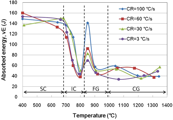
Relationship between absorbed energy and peak temperature of one-cycle

The microstructures of the simulated HAZ thermal cycle sample with the cooling rate of 60°C s⁻¹ are shown in Fig. 10. As presented in Fig. 10a, there are some big blocks in the matrix at the peak temperature of 800°C. These products are considered as M–A constituents, which explained the low absorbed energy.7^– 9 When T_p = 850°C, just higher than Ac₃ shown in Fig. 10b, the grain size became very fine, indicating the high absorbed energy in FGHAZ. However, when the perk temperature was 1350°C, the grain size grew bigger and the microstructure became to martensite and bainite, as illustrated in Fig. 10c, which explained the low absorbed energy in CGHAZ. In addition, the fractographs of the Charpy impact samples at 800 and 850°C are shown in Fig. 11. The fractograph of the sample with T_p of 800°C (ICHAZ) was characterised as brittle fracture. While in the fractograph of the sample heated to 850°C (FGHAZ), mainly dimple fracture was observed. These also explained the difference toughness in ICHAZ and FGHAZ.

Figure 10

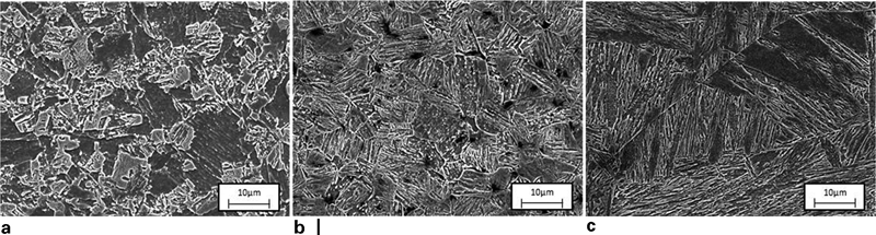
Microstructures of one-cycle specimen (CR = 60°C s⁻¹)

Figure 11

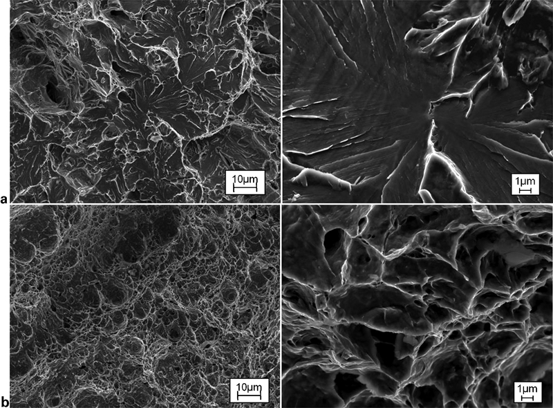
Fractography comparison of Charpy impact samples when a T_p = 800°C and b T_p = 850°C with same cooling rate of 60°C s⁻¹

Toughness database of one-cycle+temper

A new TCTP to characterise the tempering effect during multipass thermal cycles has been proposed by the authors,5 by extending the LMP to non-isothermal heat treatment. And the proposed TCTP which has been proved can be applied to evaluate quantitatively the tempering effect and the hardness change during both thermal cycle tempering processes and multipass isothermal heat treatment.5

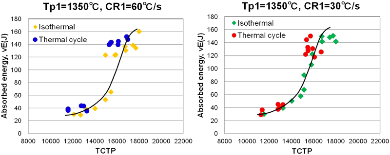
The relationship between the absorbed energy and TCTP after isothermal heat treatment and thermal cycle is illustrated in Fig. 12. With the same initial toughness (the same T_p1 and CR₁), the absorbed energy after both isothermal heat treatment and thermal cycle increased monotonously with increasing TCTP, along the same curve. It follows that the TCTP can be applied to evaluate quantitatively the tempering effect and the toughness change during both thermal cycle tempering process and multipass isothermal heat treatment. As a result, the absorbed energy after one-cycle+temper is determined by three parameters: T_p1 and CR₁ of the first thermal cycle, and TCTP of the following temper cycles.

Figure 12

Relationship between absorbed energy and TCTP after isothermal heat treatment and temper thermal cycle

Figure 13 shows the relationship between the absorbed energy and TCTP of one-cycle+temper with different values of T_p1. With increasing TCTP, the absorbed energy increased significantly for all T_p1 conditions. However, at the cooling rate of 3°C s⁻¹, the absorbed energy of the whole process is relatively lower than that with the other cooling rates.

Figure 13

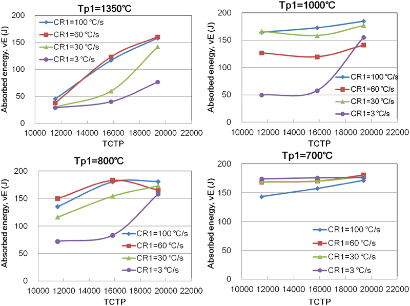
Relationship between absorbed energy and TCTP after one-cycle+temper

The microstructures of CGHAZ (T_p1 = 1350°C) before and after tempering were characterised by SEM observation as presented in Fig. 14. Before tempering, there was lath martensite structure in the matrix. While after the tempering of 1 h at 650°C, the bright interlath carbide was precipitated in the martensite structure, which explained the improvement of toughness after tempering.

Figure 14

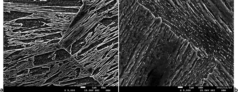
Microstructure comparison before and after tempering (one-cycle+temper, T_p1 = 1350°C, CR₁ = 100°C s⁻¹)

Toughness database of two-cycle and two-cycle+temper

There are thousands of specimens used to simulate two-cycle and two-cycle+temper in HAZ of temper bead welding, because the absorbed energy is determined by four and five parameters respectively. Figures 15 and 16 show some examples of the Charpy impact test results of two-cycle and two-cycle+temper. Because there are more than two parameters in the systems, the relationship between the absorbed energy and only two parameters are shown in each figure with the other parameters being fixed.

Figure 15

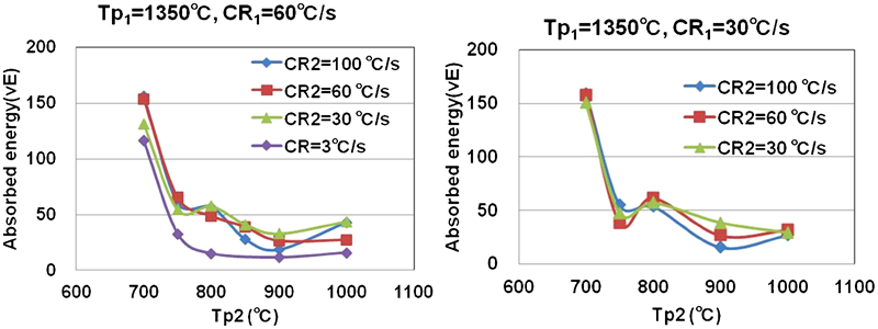
Relationship between absorbed energy and T_p2 after two-cycle

Figure 16

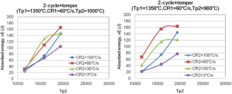
Relationship between absorbed energy and TCTP after two-cycle+temper

For example, Fig. 15a shows the relationship between the absorbed energy and T_p2/CR₂ of the second thermal cycle, when the first thermal cycle is fixed as T_p1 = 1350°C and CR₁ = 60°C s⁻¹ in the two-cycle. The embrittlement in intercritically reheated CGHAZ occurred significantly, which could be attributed to the formation of coarse necklace-like M–A constituent along the prior austenite grain boundary region and fine elongated M-A constituent within the prior austenite grain.8

The relationship between the absorbed energy and TCTP/CR₂ of two-cycle+temper is presented in Fig. 16, with the constant three parameters. It indicates that the absorbed energy increased significantly with increasing the TCTP for all conditions, attributing to the precipitation of carbide with the increasing of temper effect.

Neural network based toughness prediction subsystem

Because the toughness after all kinds of thermal cycles is determined by the parameters: T_pi, CR_i and TCTP, the prediction systems of toughness are constructed with using a Neural Network. A neural network (NN) method is a powerful tool which can process such complex data as involved in the present research.

RBF-NN

NN13, 14 is a mathematical model or computational model that simulates the structure and/or functional aspects of biological neural networks. In most cases, a NN is an adaptive system that changes its structure based on external or internal information that flows through the network during the learning phase. Modern neural networks have become useful modelling tools for non-linear statistical data. They are usually used to model complex relationships between inputs and outputs or to find patterns in data.

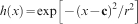
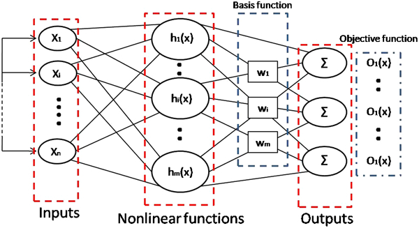
The radial basis function (RBF)15 is a powerful technique for interpolation of multidimensional space in a NN. Figure 17 illustrates the RBF-NN model. RBF networks typically have three layers: an input layer, a hidden layer with a non-linear RBF activation function and a linear output layer. The hidden layer can be described by a Gaussian basis function (6) where x is the input data, c is the centre vector and r is the Euclidean distance. In the basic form all inputs are connected to each hidden neuron.

Figure 17

Radial basis function neural network model

The output O(x_i) of the network is thus (7) where n is the number of neurons in the hidden layer, c_j is the centre vector for neuron j, and w_j are the weights of the linear output neuron. The weights w_j, c_j and r are determined in a manner that optimises the fit between O(x_i) and the data.

Prediction subsystem of toughness

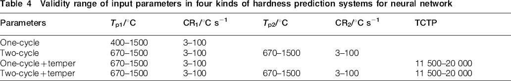
In the present study, the thermal cycle parameters (for example, T_pi, CR_i and TCTP of the tempering thermal cycle) are the input data, and the toughness is the output data. The validity range of the input parameters for neural network is shown in Table 4. There are only two input parameters in one-cycle subsystem, but there are three, four and five input parameters in one-cycle+temper, two-cycle and two-cycle+temper subsystems respectively. Thus, the main question is the determination of w_i, c_i and r, which depend on practical experimental results. Based on the experimental results, the thermal cycle parameters (such as T_pi, CR_i and TCTP) and toughness data were fed into the RBF-NN, and as a result, w_i, c_i and r were determined. It should be noted that every input data set has produced one weight w_i; therefore, thousands of weights w_i have been produced according to the thousands of experimental results. By using these obtained constants, the toughness prediction subsystem for multipass thermal cycles was constructed.

Table 4

Validity range of input parameters in four kinds of hardness prediction systems for neural network

Parameters	T_p1/°C	CR₁/°C s⁻¹	T_p2/°C	CR₂/°C s⁻¹	TCTP
One-cycle	400–1500	3–100
Two-cycle	670–1500	3–100	670–1500	3–100
One-cycle+temper	670–1500	3–100			11 500–20 000
Two-cycle+temper	670–1500	3–100	670–1500	3–100	11 500–20 000

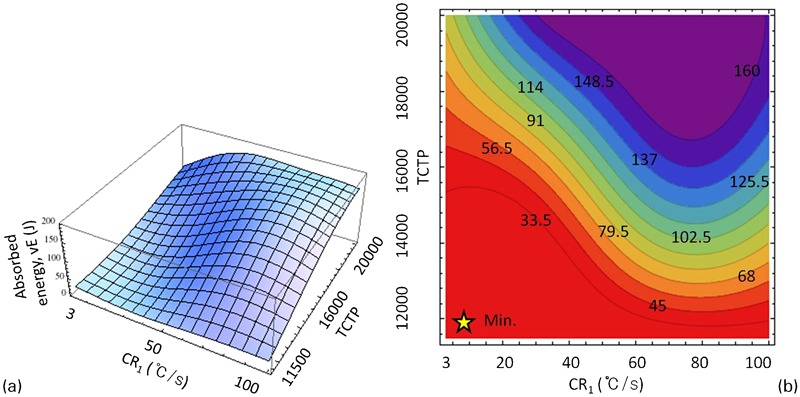
Based on plentiful experimental results, the toughness prediction subsystem for the four types of thermal cycle pattern has been constructed, as illustrated in Figs. 18–21. Figure 18 represents the calculated 3D and 2D contour figures of the complex relationship between toughness and T_p/CR for one-cycle. In the 2D contour figure of Fig. 18b, different toughness ranges are shown in different colours. The star mark indicates the lowest toughness, which occurred in CGHAZ with the lowest cooling rate of 3°C s⁻¹ because of the large grain size formed at the low cooling rate. Furthermore, an valley appears in the range between 700 and 800°C, indicating that toughness in ICHAZ (Ac₁–Ac₃) has decreased possibly caused by the presence of M–A constituents.8^– 10 With this prediction subsystem of one-cycle, as shown in Fig. 18, the toughness of low alloy steel A533B subjected to any single thermal cycle can be calculated if the T_p and CR of the thermal cycle process are known.

Figure 18

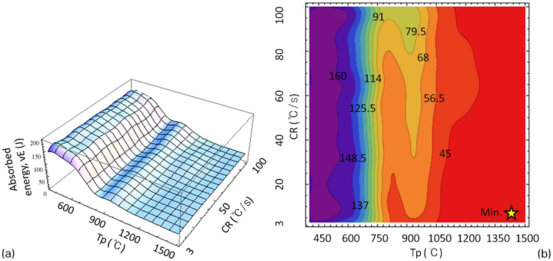
Toughness prediction system of one-cycle

Figure 19

Toughness prediction system of two-cycle when T_p1 = 1350°C and CR₁ = 3°C s⁻¹

Figure 20

Toughness prediction system of one-cycle+temper with constant T_p1 = 1350°C

Figure 21

Toughness prediction of two-cycle+temper when T_p1 = 1350°C, CR₁ = 90°C s⁻¹ and T_p2 = 750°C

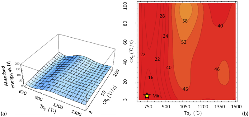
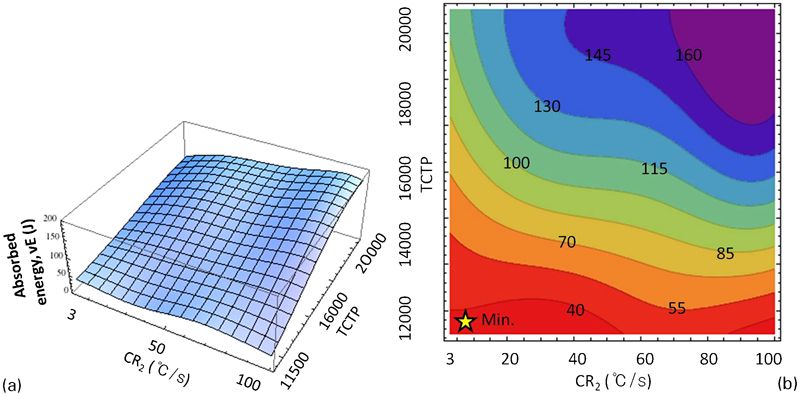
Figure 19 shows an example of the toughness prediction subsystem for a double thermal cycle (two-cycle). In this subsystem, there are four input parameters: T_p1 and CR₁ of the first thermal cycle, and T_p2 and CR₂ of the second thermal cycle. Together with the output toughness, it is a five-dimensional space. To enable visualisation of the results, two of these parameters must be fixed. Figure 19 shows the 3D and 2D contour relationship figure between toughness and T_p2/CR₂ of the second thermal cycle, when T_p1 and CR₁ of the first thermal cycle are fixed at 1350°C and 3°C s⁻¹ respectively. Here, all the 2D contour figures use the same colour–toughness scale. These data show that the loss in toughness always occurred in ICCGHAZ.9

Figure 20 presents an example of the toughness prediction subsystem for a one-cycle+temper thermal cycle. There are three variable parameters: T_p1 and CR₁ of the first thermal cycle, and TCTP of the following temper thermal cycles with the peak temperature between 400 and 670°C. The relationship between toughness and CR₁/TCTP is shown in Fig. 20, with a constant T_p1 of 1350°C. With decreasing CR₁ and TCTP, toughness of the simulated CGHAZ decreased. As a result, the valley value of vE appeared with the lowest CR₁ and the lowest TCTP.

Among these four toughness prediction subsystems, the two-cycle+temper thermal cycle is the most complicated for toughness prediction. In this subsystem, five parameters have been included: T_p1 and CR₁ of the first thermal cycle, T_p2 and CR₂ of the second thermal cycle, and TCTP of the following temper thermal cycles. Therefore, three parameters need to be fixed for visualisation of the results. Figure 21 shows the relationship between toughness and CR₂/TCTP, when T_p1/CR₁ of the first thermal cycle and T_p2 of the second thermal cycle are fixed.

Using these four types of toughness prediction subsystems, the toughness of A533B can be calculated when the thermal cycle parameters are known. Based on any thermal cycles measured in the experiments or calculated by FEM simulation, the toughness after the thermal cycles can be calculated.

Effectiveness of toughness prediction subsystem

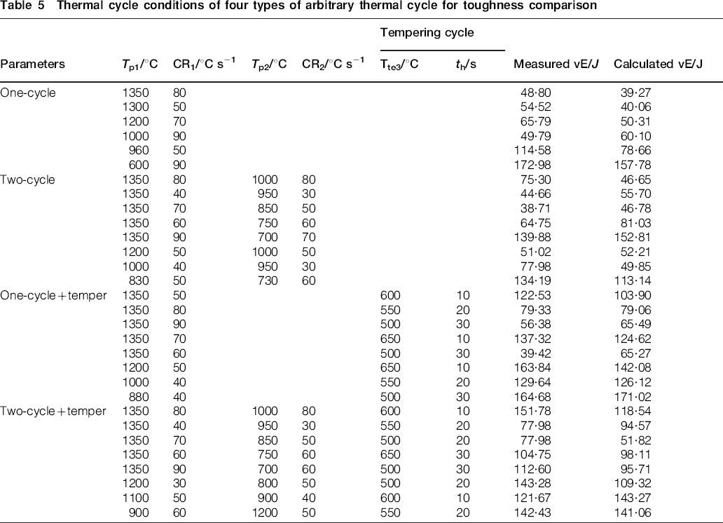
In order to verify the effectiveness of the toughness prediction subsystem, samples heated with arbitrary thermal cycles by Gleeble 1500 have been used to investigate the toughness. The details of the arbitrary thermal cycle conditions are shown in Table 5. Thirty thermal cycles were chosen, which included six one-cycle, and eight two-cycle, one-cycle+temper and two-cycle+temper respectively.

Table 5

Thermal cycle conditions of four types of arbitrary thermal cycle for toughness comparison

Parameters	T_p1/°C	CR₁/°C s⁻¹	T_p2/°C	CR₂/°C s⁻¹	Tempering cycle		Measured vE/J	Calculated vE/J
Parameters	T_p1/°C	CR₁/°C s⁻¹	T_p2/°C	CR₂/°C s⁻¹	T_te3/°C	t_h/s	Measured vE/J	Calculated vE/J
One-cycle	1350	80					48·80	39·27
	1300	50					54·52	40·06
	1200	70					65·79	50·31
	1000	90					49·79	60·10
	960	50					114·58	78·66
	600	90					172·98	157·78
Two-cycle	1350	80	1000	80			75·30	46·65
	1350	40	950	30			44·66	55·70
	1350	70	850	50			38·71	46·78
	1350	60	750	60			64·75	81·03
	1350	90	700	70			139·88	152·81
	1200	50	1000	50			51·02	52·21
	1000	40	950	30			77·98	49·85
	830	50	730	60			134·19	113·14
One-cycle+temper	1350	50			600	10	122·53	103·90
	1350	80			550	20	79·33	79·06
	1350	90			500	30	56·38	65·49
	1350	70			650	10	137·32	124·62
	1350	60			500	30	39·42	65·27
	1200	50			650	10	163·84	142·08
	1000	40			550	20	129·64	126·12
	880	40			500	30	164·68	171·02
Two-cycle+temper	1350	80	1000	80	600	10	151·78	118·54
	1350	40	950	30	550	20	77·98	94·57
	1350	70	850	50	500	20	77·98	51·82
	1350	60	750	60	650	30	104·75	98·11
	1350	90	700	60	500	30	112·60	95·71
	1200	30	800	50	500	20	143·28	109·32
	1100	50	900	40	600	10	121·67	143·27
	900	60	1200	50	550	20	142·43	141·06

The toughness of the samples after the arbitrary thermal cycles being applied is compared with the calculated results by the previously mentioned NN based toughness prediction subsystem, as illustrated in Fig. 22. The y coordinate presents the experimentally measured absorbed energy vE, and the x coordinate shows the calculated ones. It can be found that there is a good agreement between the calculated absorbed energy and the measured one. This result indicates that the toughness of the steel after any thermal cycles being applied, which may occur in HAZ of temper bead welding, can be calculated using the proposed toughness prediction subsystem when the thermal cycle parameters are known.

Figure 22

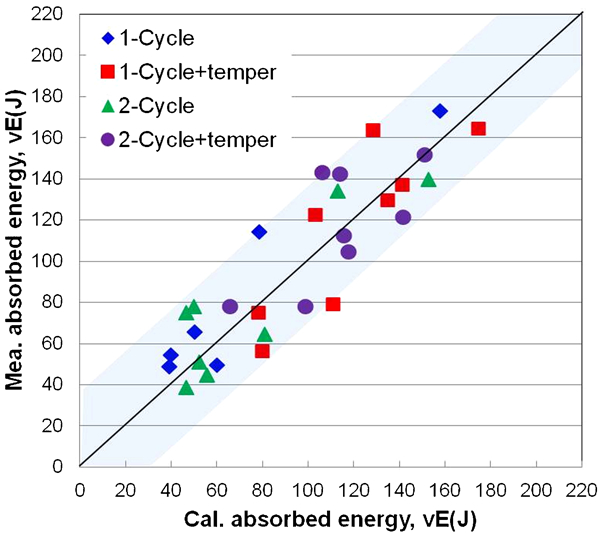
Comparison between measured and calculated toughness of arbitrary thermal cycles

Toughness prediction system in HAZ of temper bead welding

Toughness prediction system for temper bead welding

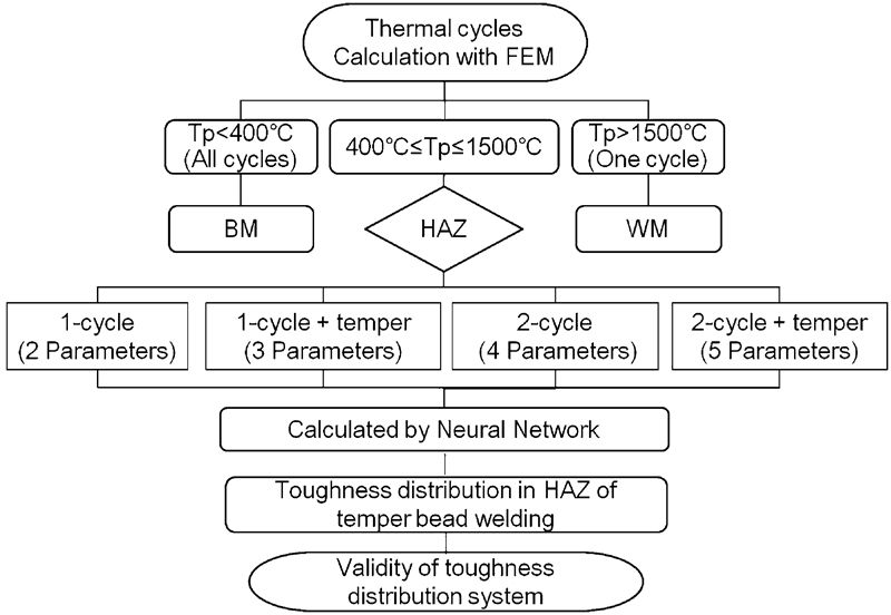
Figure 23 shows the whole toughness prediction system in HAZ of temper bead welding, which includes following subsystems. First, the thermal cycles in HAZ of temper bead welding are simulated by FEM. Second, the base metal (BM), HAZ and the weld metal (WM) were judged according to the peak temperatures of the simulated multi-pass thermal cycles. If all the peak temperatures of the multipass thermal cycle are lower than 400°C, the grid node is considered as BM. If any peak temperature is over 1500°C, then the grid node is classified as WM. All other nodes, with at least one peak temperature during the thermal cycles between 400 and 1500°C, are considered to be HAZ, which is the target region to be calculated. Within this part of the data, according to the thermal history, the thermal cycles of the grid nodes are also classified into four types: one-cycle, one-cycle+temper, two-cycle and two-cycle+temper. Third, the thermal cycle parameters (T_pi, CR_i and TCTP) will be fed into the proposed NN based prediction subsystem, and the toughness at every grid node is calculated. It should be noted that for the multipass thermal cycles with temper thermal cycles, the TCTP of the temper thermal cycles is calculated before feeding into the NN prediction subsystem. Fourth, according to the calculated toughness of every grid node, the visual toughness distribution in HAZ of temper bead welding can be shown as colour charts using Mathematica software. Finally, the predicted toughness is compared with the experimentally measured one to verify the effectiveness of the toughness prediction system.

Figure 23

Toughness prediction system for temper bead welding

Temperature analysis in HAZ of temper bead welding by FEM

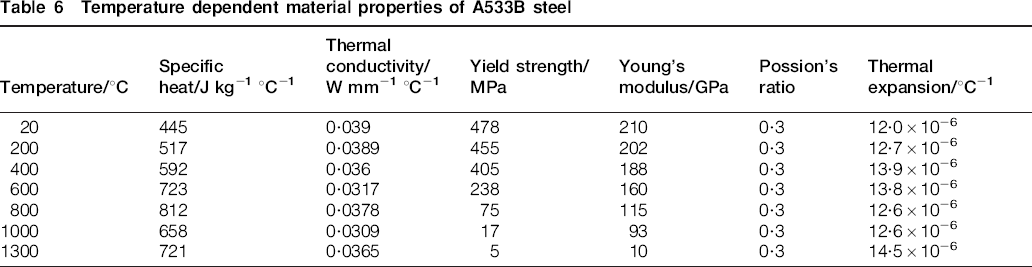
The temperature distributions produced by multi-pass thermal cycles in welds during temper bead welding were calculated using 3D finite element analysis code, developed specifically for welding simulation. The mesh model is shown in Fig. 24, which is the same size with the experimental welding sample. The notch positions of the side notched Charpy samples are shown in red lines of P1–P5, with different distances far from the bead line. The mesh near the WM is finer than that in BM. The temperature dependent physical properties of A533B are illustrated in Table 6. The welding conditions were the same as the experimental conditions shown in Table 3, which followed the consistent layer technique. Figure 25 presents the calculated peak temperature distribution in the middle section of seven-layer–88-pass welds. Different peak temperatures are presented in different colours.

Figure 24

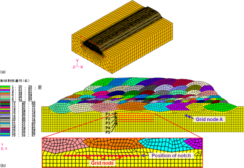
Mesh model for FEM analysis (seven-layer–88-pass welding)

Figure 25

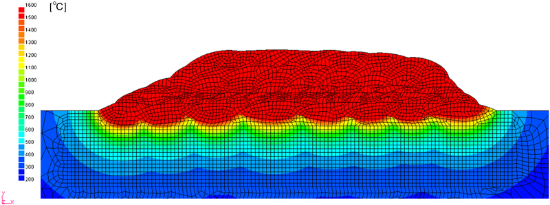
Simulated peak temperature distribution of seven-layer–88-pass welding

Table 6

Temperature dependent material properties of A533B steel

Temperature/°C	Specific heat/J kg⁻¹ °C⁻¹	Thermal conductivity/W mm⁻¹ °C⁻¹	Yield strength/MPa	Young's modulus/GPa	Possion's ratio	Thermal expansion/°C⁻¹
20	445	0·039	478	210	0·3	12·0×10⁻⁶
200	517	0·0389	455	202	0·3	12·7×10⁻⁶
400	592	0·036	405	188	0·3	13·9×10⁻⁶
600	723	0·0317	238	160	0·3	13·8×10⁻⁶
800	812	0·0378	75	115	0·3	12·6×10⁻⁶
1000	658	0·0309	17	93	0·3	12·6×10⁻⁶
1300	721	0·0365	5	10	0·3	14·5×10⁻⁶

Toughness calculation based on simulated thermal cycles

As explained in the section on ‘Toughness prediction system for temper bead welding’, according to the thermal history, the simulated thermal cycles of the grid nodes in HAZ are also classified into four types: one-cycle, one-cycle+temper, two-cycle and two-cycle+temper. And then, the thermal cycle parameters are fed into the proposed NN based prediction subsystem, and the toughness at every grid node is calculated.

Figure 26 illustrates an example of toughness calculation based on a multipass thermal cycle at grid node A in Fig. 24b. In these thermal cycles, there are two-pass thermal cycles with a peak temperature higher than Ac₁, followed by multipass temper thermal cycles with the peak temperature between 400°C and Ac₁. It should be noted that the first thermal cycle with peak temperature lower than 400°C is disregarded in the calculation, because it has little effect on the toughness. Thus, this multipass thermal cycle can be calculated as two-cycle+temper type. First, the TCTP of the temper thermal cycles is calculated, and then T_p1/CR₁ of the first thermal cycle, T_p2/CR₂ of the second thermal cycle and the calculated TCTP five parameters are input into the toughness prediction subsystem for two-cycle+temper constructed from the NN, and the toughness is calculated. Using this method, the toughnesses in all positions of the HAZ can be predicted using the four different toughness prediction subsystems.

Figure 26

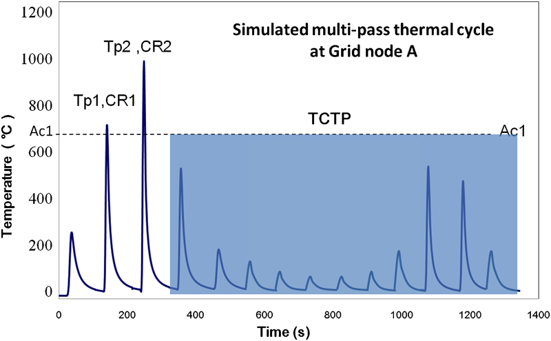
Toughness calculation based on simulated multipass thermal cycle at Grid node A in Fig. 24b

Predicted toughness distribution of temper bead welding

Based on the calculated thermal history of every grid node, the toughness at the grid node was also calculated using the proposed NN based toughness prediction systems. The visual toughness distribution in the HAZ is shown as colour chart maps in Fig. 27 using the Mathematica software. Besides the red WM and grey BM regions, the toughness in the HAZ is shown with rainbow colours according to the different toughness levels. It shows that the low toughness appeared in the CGHAZ near to WM. And the absorbed energy in the whole HAZ region is higher than 40 J (the required specification in industry) after the temper bead welding.

Figure 27

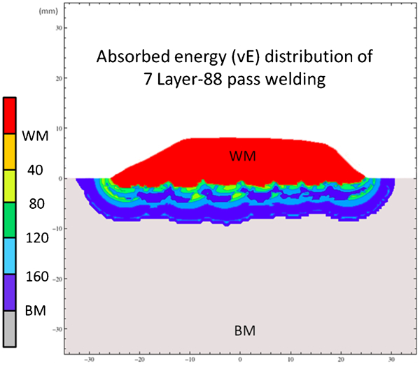
Calculated toughness distribution in HAZ of seven-layer–88-pass welding based on FEM analysis

Validity of toughness prediction system

The predicted toughness and the experimentally measured results for the HAZ of A533B low alloy steel after seven-layer–88-pass welding are shown in Fig. 28. The notch of the Charpy impact sample is in HAZ region of temper bead welded sample using the method illustrated in Fig. 7. The red points are the experimentally measured toughness, and the blues points are the calculated toughness using our NN based toughness prediction systems, based on the FEM simulated thermal history. The calculated toughness was obtained as the average toughness of 20 calculated values according to the mixing rules, which is employed rather successfully, especially for calculating elastic and thermal properties.16^– 19 The predicted toughness is in good accordance with the experimentally measured toughness, and both the predicted absorbed energy and the measured one are higher than 40 J. It follows that the proposed system for toughness prediction is useful and effective at estimating the tempering effect in temper bead welding.

Figure 28

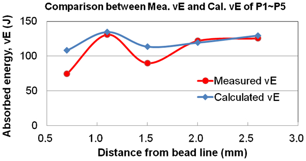
Relationship between measured and calculated absorbed energy according to distance from bead line (P1–P5 shown in Fig. 24b)

In sum, through the above method, the toughness can be predicted before the actual temper bead welding. If the calculated toughness in HAZ is lower than 40J (it means it cannot fit the required specification in industry), the welding conditions would be modified. Thus, the appropriate welding conditions can be selected before the actual welding. It is useful for the repair welding for the large structures.

Conclusions

A NN based system for toughness prediction in the HAZ of low alloy steel when temper bead welding is applied has been investigated. The following conclusions can be drawn:

The NN based subsystem for toughness prediction was constructed based on the experimentally obtained database.

On the basis of the FEM simulated thermal cycle parameters, the toughness distribution in HAZ of temper bead welding was predicted using the NN prediction system.

The predicted toughness was found to be in good accordance with the experimentally measured results. It follows that the proposed toughness prediction system is effective for estimating the tempering effect in temper bead welding.

References

Yurioka

, Horii

: ‘Recent developments in repair welding technologies in Japan’, Sci. Technol. Weld. Join., 2006, 11, 255–264.

Nakao

, Oshige

, Noi

, Nishi

: ‘Distribution of toughness in HAZ of multi-pass welded high strength steel’, Q. J. Jpn Weld. Soc., 1985, 3, 773–781.

Mizuno

, Brziak

, Lomozik

, Matsuda

: ‘Appropriate welding conditions of temper bead weld repair for SQV2A pressure vessel steel’, Proc. 30th MPA-Sem. in conjunction with the 9th German-Japanese Sem., Stuttgart, Germany, October 2004, MPA, 7·1–7·9.

Deng

, Murakawa

: ‘Prediction of welding residual stress in multi-pass butt-welded modified 9Cr–1Mo steel pipe considering phase transformation effects’, Comput. Mater. Sci., 2006, 37, 209–219.

, Nakabayashi

, SaSa

, Itoh

, Kameyama

, Hirano

, Chigusa

, Saida

, Mochizuki

, Nishimoto

: ‘Neural network prediction of hardness in HAZ of temper bead welding using the proposed thermal cycle tempering parameter (TCTP)’, ISIJ Int., 2011, 51, 1506–1515.

Yurioka

, Horii

: ‘Recent developments in repair welding technologies in Japan’, Sci. Technol. Weld. Join., 2006, 11, 255–264.

Viswanathan

, Gandy

, Findlan

: ‘Temper bead welding of P-Nos. 4 and 5 materials’, EPRI TR-111757, EPRI, Palo Alto, CA, USA, December 1998.

Matsuda

, Ikeuchi

, Liao

: ‘Weld HAZ toughness and its improvement of low alloy steel SQV-2A for pressure vessels (Report 1)’, Trans. JWRI, 1993, 22, 271–279.

Matsuda

, Ikeuchi

, Liao

: ‘Weld HAZ toughness and its improvement of low alloy steel SQV-2A for pressure vessels (Report 2)’, Trans. JWRI, 1994, 23, 49–57.

10.

Liao

, Ikeuchi

, Matsuda

: ‘Weld HAZ toughness and its improvement of low alloy steel SQV-2A for pressure vessels (Report 3)’, Trans. JWRI, 1994, 23, 223–230.

11.

Deng

, Murakawa

, Shibahara

: ‘Investigations on welding distortion in an asymmetrical curved block by means of numerical simulation technology and experimental method’, Comput. Mater. Sci., 2010, 48, 187–194.

12.

Bayraktar

, Hugele

, Jansen

, Kaplan

: ‘Evaluation of pipeline laser girth weld properties by Charpy (V) toughness and impact tensile tests’, J. Mater. Process. Technol., 2004, 147, 155–162.

13.

Manvatkar

, Arora

, De

, DebRoy

: ‘Neural network models of peak temperature, torque, traverse force, bending stress and maximum shear stress during friction stir welding’, Sci. Technol. Weld. Join., 2012, 17, 460–466.

14.

Metzbower

, Olson

, Yurioka

: ‘Neural network analysis of oxygen in weld metals’, Sci. Technol. Weld. Join., 2009, 14, 566–569.

15.

Casasent

, Chen

: ‘Radial basis function neural networks for nonlinear Fisher discrimination and Neyman–Pearson classification’, Neural Networks, 2003, 16, 529–535.

16.

Hartwig

: ‘Polymer properties at room and cryogenic temperatures’, International Cryogenics Monograph Series; 1995, New York, Plenum.

17.

Grellmann

, Seidler

: ‘Deformation and fracture behaviour of polymers’; 2001, Berlin, Springer.

18.

Solorzano-Zavala

, Barragan-Aroche

, Bazua

: ‘Comparative study of mixing rules for cubic equations of state in the prediction of multicomponent vapour–liquid equilibria’, Fluid Phase Equilib., 1996, 122, 99–116.

19.

Valderrama

, Alvarez

: ‘Temperature independent mixing rules to correlate the solubility of solids in supercritical carbon dioxide’, J. Supercrit. Fluids, 2004, 32, 37–46.