Finite element simulation of butt welded 2·25Cr–1·6W steel pipe incorporating bainite phase transformation

Abstract

This article presents a newly developed global optimisation method for the finite element simulation of welding process considering bainite transformation. In this method, the pattern search algorithm was applied to determine kinetic parameters in Johnson–Mehl–Avrami–Kolmogorov (JMAK) equation during a continuous cooling process. Meanwhile, the JMAK equation was modified into an explicit form as a function of welding temperature field to improve calculation efficiency in the optimisation process. This methodology improves the accuracy as calculating the temperature dependent volume fraction of bainite transformation in finite element simulation. The calculated welding residual stresses considering phase transformation effects exhibited better agreement with the measured results than those calculated without phase transformation. The influences of variable cooling rates on welding residual stresses were also investigated.

Keywords

Welding residual stress Pattern search method Finite element modelling Bainite transformation Optimisation

Introduction

Welding induced residual stress mainly results in brittle fracture, buckling deformation and stress corrosion cracking, and reduces the fatigue life of welded structures in service. Accurate prediction and quantitative estimation of welding residual stresses are of significant interest to the safety of the structures. It has been recognised that solid state phase transformation during cooling can significantly affect the development of residual stresses in steel welds.1^– 3

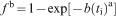
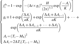
For the diffusional phase transformation, many researchers have used the Johnson–Mehl–Avrami–Kolmogorov (JMAK) equation to predict the change of phase volume fraction during continuous cooling.1,4^– 10 The JMAK equation was given by (1) where f^b is the volume fraction of bainite, and t is time. Kinetic parameters b and a are usually obtained in isothermal conditions over a range of temperatures.1,9^– 11 Although the JMAK equation is obtained from the isothermal solution, it constitutes the basis for analysing phase transformation under non-isothermal condition.12 Garcia et al. 13, 14 developed a mathematical model to produce the kinetics of the pearlite–austenite transformation in a eutectoid steel during continuous heating. This model considered the influence of structural parameters, such as interlamellar spacing and edge length of pearlite colonies. Some researchers indicated that the parameters obtained by Garcia et al. can only be used for specific microstructure whose grain size and interlamellar spacing lie along a straight line.12 Tszeng and Shi11 developed an algorithm to identify the kinetics of diffusional phase transformations from dilatometry data. The fundamental parameters governing the nucleation and growth of the new phase were determined by minimising the error between the measured dilatometry curves and that calculated by the prespecified kinetic model. However, some important parameters were obtained from the knowledge of crystallography of each phase and the data of lattice parameters depending on temperature and composition.15 Therefore, this method cannot be applied to steel that lack such parameters. The JMAK model with Scheil's additivity rule has been widely used to investigate the effects of bainite transformation during quenching and welding process.9, 10 Scheil's additive rule describes a non-isothermal cooling process by subdividing the cooling curve into various small isothermal steps.9 In this method, the kinetic parameters in JMAK model were calculated by a couple of volume fractions at a specified temperature from the time–temperature–transformation diagrams. If two different sets of percentiles were used to regress the parameters in JMAK, the results would be deviated from each other. Furthermore, in finite element (FE) simulation, the volume fraction of bainite phase is strongly sensitive to the increment time and the total number of increments during phase transformation process. Especially, with the identical kinetic parameter, different FE computational conditions would result in disparate phase fractions.

Pattern search method is widely used to determine the parameters for optimisation problems, especially when the formulas are in complicated forms. This method is characterised by a series of exploratory moves, which consider the behaviour of the objective function at a pattern of points, all of which lie on a rational lattice.16 Moreover, the pattern search inherits some properties of the imported global optimisation technique, without jeopardising the convergence for local stationarity.17

This paper presents a new numerical optimisation method based on pattern search algorithm to determine the parameters in JMAK equation. Meanwhile, in order to improve the efficiency of global optimisation process, the JMAK equation was modified to an explicit form. Finally, FE simulation for the welding process of butt welded 2·25Cr–1·6W steel pipes was performed using the optimisation technique. The temperature and residual stress calculated from FE simulation were compared with experimental results. The effects of the cool rates on residual stress were also analysed in detail.

Numerical implementation of JMAK equation

Transformation experiment

Cylindrical specimens with 4 mm in diameter and 10 mm in length were prepared for dilatometric tests to measure transformation strains. Dilatometric specimens were heated to 1050°C at a rate of 100°C min⁻¹ and held for 10 min to assure complete austenitising,18 followed by continuous cooling to room temperature at rates ranging from 1 to 30°C s⁻¹. The 2·25Cr–1·6W steel can be completely converted to bainite phase in such range of cooling rates.19 In actual welding process, the cooling rate in the air cooling condition is between 1 and 10°C s⁻¹ contained in the rate range of this experiment. Figure 1 shows the dilatometric curves. It is seen that the expansion occurs at temperatures between 450 and 600°C during cooling. Owing to the nonlinear relationship, the increase in transformation strain is gradually larger when temperature drifts lower at the beginning of phase transformation. For all cooling rates, the phase transformation process is related to bainitic transformation. Different cooling rates have resulted in a change of B_s as well as of volumetric strain listed in Table 1.

Figure 1

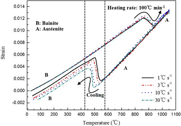
Dilatometric curve of 2·25Cr–1·6W steel at cooling rates of 1–30°C s⁻¹

Table 1

B_s, volumetric strain of bainite–austenite and austenite–bainite transformation at different cooling rates

Cooling rate/°C s⁻¹	B_s/°C	Volumetric strain of bainite–austenite	Volumetric strain of austenite–bainite
1	547	−2·65×10⁻³	4·68×10⁻³
3	536	−2·84×10⁻³	4·68×10⁻³
10	517	−2·79×10⁻³	4·49×10⁻³
30	494	−2·76×10⁻³	3·92×10⁻³

Determination of kinetic parameters in JMAK equation

Most researchers used JMAK equation to describe bainite phase transformations.1, 9, 10 The parameter a in equation (1) is often assumed to be temperature independent.20 The parameter b was fitted to a modified Gaussian distribution function depending on temperature.10 Therefore, the JMAK equation can be expressed as (2) where indicates volume fraction of the bainite phase in the ith time step, time increment Δt_i is assumed to be constant and is a fictitious time.10

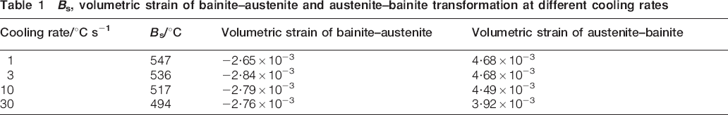
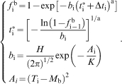
The pattern search method was then used to identify the optimal H and K. As shown in equation (2), the calculation of is actually an iterative process. By transforming equation (2) into explicit form as a function of temperature (see Appendix), the efficiency of pattern search method would be improved significantly. The explicit equations are derived as (3) For the sequentially coupled thermal–mechanical FE simulation, A_i and ΔA_i can be obtained from transient temperature fields resulting from thermal analysis.

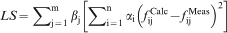
According to the dilatation curves in Fig. 1, the temperature dependent bainite volume fraction curves (Fig. 2) under the various cooling rates were obtained,21 which were the objective curves in pattern search method. The errors between measured and calculated curves are summarised into a least square function (4) where m is the number of elements, n is the number of points on the curve j, α_i and β_j are the scaling factors and are used to guide the optimisation process and the superscripts Calc and Meas denote the calculated and measured phase transformation volume fraction values respectively.

Figure 2

Temperature dependent bainite transformation volume fraction curves

Welding simulation

Finite element model

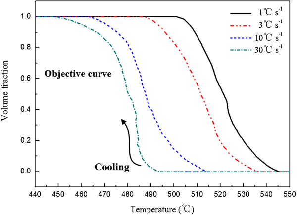
A sequentially coupled thermal–mechanical FE analysis was performed based on ABAQUS. The material used in this study was 2·25Cr–1·6W steel pipes with an outer diameter of 56 mm, thickness of 13 mm and length of 100 mm. The pipe was welded by a multipass welding process. Because of symmetry, one half of the structure was modelled. The 3D FE model with 33040 eight-node hexahedral elements is shown in Fig. 3. The FE mesh was refined in the weld bead and heat affected zone with element size between 0·5 and 1·5 mm to assure that the molten zone can cover at least 5×4×3 elements (length×width×depth), which can assure that more accurate simulated results can be obtained. The model in this study adopted the technique of element ‘birth and death’ to simulate the weld filler. Meanwhile, the heat transfer and constraint boundary conditions were also modified after the new elements were added. The temperature dependent thermal mechanical properties of the 2·25Cr–1·6W steels are shown in Fig. 4.

Figure 3

Finite element model

Figure 4

Temperature dependent thermal and mechanical properties

Thermal analysis

In thermal analysis, a moving double ellipsoidal volumetric heat source22 was applied to model heat input. The fluid flow of material cannot be directly considered because coupled solid–liquid problem is not involved in ABAQUS. If the effect of the fluid flow is neglected, the highest temperature in weld pool will be >3000°C when the double ellipsoidal heat source model is used.23 This phenomenon is much different from the realistic situation. Okagaito et al. 24 suggest that the highest temperature on the molten pool surface is ∼1750°C. In this study, the thermal conductivity above the melting temperature was assumed to be twice as that of room temperature.23

Generally, the weld shape is also controlled by heat transfer because of a combination of convection and conduction in the liquid pool. The heat transfer in the weld pool is dominated by conduction for Pe<<1.25, 26 The welding speed in this study was 5 mm s⁻¹. It meant that it was a rapidly travelling heat source. Therefore, the heat transfer in the liquid pool was dominated by the transverse conduction.27

The thermal effects due to solidification are modelled by considering the latent heat for fusion. The value of the latent heat is 270 J g⁻¹.10 The liquidus and solidus temperature are 1500 and 1460°C respectively. To account for heat losses, both the thermal radiation and heat transfer on surface were modelled. The preheating and interpass temperature were assumed to be 150°C.

Mechanical analysis

The mechanical analysis was conducted using the temperature distributions calculated by the thermal analysis as the input thermal loading. In this model, the stress versus strain curve was assumed to be expressed by linear kinematic hardening.

Austenitic transformation occurs during heating at a relatively high temperature (820–950°C). The mechanical properties are weak at such high temperatures. Therefore, the influence of austenitic transformation on stresses is relatively smaller than that of bainite transformation. A linear relation was assumed to estimate the increment of austenite volume fraction, as follows10 (5) The modified JMAK equations were used to describe the bainite transformation. The parameters H and K were obtained by the global optimisation method mentioned above.

In this study, transformation induced plasticity was not taken into account. Ignoring this component, the strain increment can be then expressed by the following equation (6) The increment of volumetric strain at the ith step during the bainite transformation process can be determined by the following equation (7)

Results and discussion

Temperature results

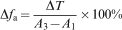
The temperature history of experiment and simulation is compared for the position of weld toe in Fig. 5. It is obvious that the results have generally good conformity, but the difference between the results is noticeable at the beginning of temperature rise stage. It is probably due to molten spattering during fusion welding and the selection of heat source model. The calculated highest temperature of the weld pool is ∼1800°C, which is much closer to the realistic situation.23, 24

Figure 5

Measured and calculated temperature history at weld toe

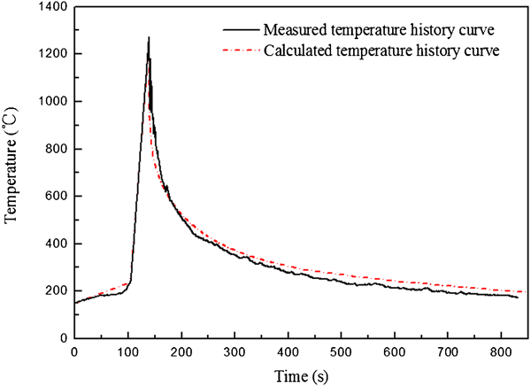
Figure 6 shows calculated and measured cooling curves at various positions in temperature range of 450–550°C. Bainite transformation of 2·25Cr–1·6W occurs in such temperature range. It is observed that the cooling rates are almost similar and keep 3°C s⁻¹ in different positions, which is attributed to small size of the pipe. Therefore, we can use the unique set of H and K to calculate phase transformation during a thermal cycle.

Figure 6

Calculated cooling curves versus measured cooling curve

Welding residual stress results

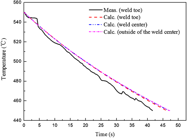
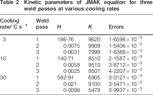
The kinetic parameters obtained by pattern search method are listed in Table 2. All errors are within the specified tolerance of 0·5%. Figures 7 and 8 show the hoop and axial residual stresses on the outside surface at a cooling rate of 3°C s⁻¹ calculated by two different cases, with and without considering solid state phase transformation effects respectively. The stress profiles are reported as a function of axial distance from the weld centreline. From the results, it can be observed that residual stresses calculated by those two models show similar trends. Within and near the weld area, the axial and hoop residual stresses are compressive. It is due to circumferential strain brought by the radial expansion and subsequent contraction. The circumferential shrinkage in the vicinity of the weld generates bending moment.28 Comparing with experimental results, residual stresses predicted by the model with phase transformation were much closer to measured values than those without phase transformation. Compressive stresses calculated by the case with phase transformation were much lower than those without phase transformation. The lower stresses can be explained by the volumetric increase in the material that undergoes the austenite–bainite phase transformation. The results reveal that the final welding residual stresses in 2·25Cr–1·6W steel pipes are significantly affected by volumetric change brought by bainite transformation.

Figure 7

Hoop stress distribution on outside surface

Figure 8

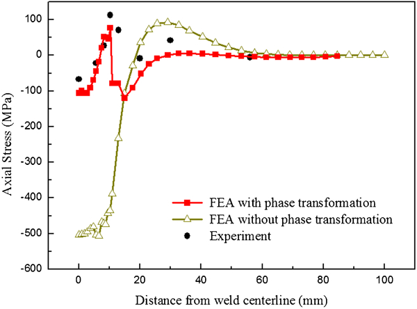
Axial stress distribution on outside surface

Table 2

Kinetic parameters of JMAK equation for three weld passes at various cooling rates

Cooling rate/°C s⁻¹	Weld pass	H	K	Errors
3	1	186·76	9620	1·6598×10⁻³
	2	0·0075	9909	1·5406×10⁻³
	3	0·0031	7999	1·6388×10⁻³
10	1	140·71	8510	2·1587×10⁻³
	2	0·0058	9510	3·8712×10⁻³
	3	0·0025	9501	4·2207×10⁻³
30	1	582·91	6905	3·0121×10⁻³
	2	0·021	9100	3·5471×10⁻³
	3	0·0098	5478	3·9937×10⁻³

Results are presented for the investigation of the various cooling rates effects. Welding started at circumferential angle θ = 0° and ended at the same location. Figure 9 shows the axial residual stresses at circumferential angle θ = 225°, distribution on the outside surface away from the weld centreline, at different cooling rates. It can be seen that at weld centre, the axial residual stresses at low cooling rate are larger than those at high cooling rate as shown in Fig. 11. This is because that strain increment of bainite transformation decreases with the increasing cooling rate plotted in Fig. 11. For the hoop residual stresses, it can be observed in Fig. 10 that the effects of various cooling rates are very small.

Figure 9

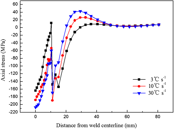
Axial stress at circumferential angle θ = 225° on outside surface

Figure 10

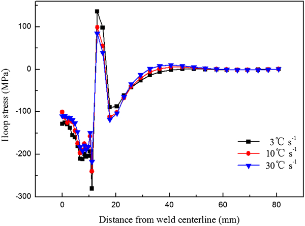
Hoop stress at circumferential angle θ = 225° on outside surface

Figure 11

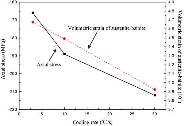
Variations in axial stresses at weld centre and volumetric strain of austenite–bainite transformation with cooling rate

Conclusions

Based on the pattern search algorithm, a global optimisation methodology was developed to accurately determine kinetic parameters in the JMAK equation. The JMAK equation was changed from an iterative form into an explicit expression to improve calculation efficiency.

The values of B_s and bainite transformation strains of 2·25Cr–1·6W, measured from the dilatometric curves at different cooling rates, separately decreased with increasing cooling rates. The bainite volume fraction curves of 2·25Cr–1·6W at different cooling rates were measured and used as objective curves in pattern search method. The kinetic parameters in JMAK model were obtained for multipass butt welded of 2·25Cr–1·6W steel pipes by the optimisation method.

Finite element simulation using the newly developed optimisation technique was performed to calculate welding residual stresses in multipass butt weld of 2·25Cr–1·6W steel pipes. The axial and hoop stresses with solid state phase transformation effects on outside surface showed much better agreement with the measured results than those calculated without solid state phase transformation. In addition, through the comparison of residual stresses at various cooling rates, it was apparent that the residual stresses were greatly influenced by volumetric change of bainite transformation.

Footnotes

Acknowledgements

This work was supported by the National Natural Science Foundation of China (Grant Nos. 50975176 and 51105251) and National Science and Technology Major Project (No. 2012ZX04010-091).

Appendix

This paper is part of a special issue on computed-aided welding engineering

References

, DebRoy

: ‘A perspective on residual stresses in welding’, Sci. Technol. Weld. Join., 2011, 16, 204–208.

Francis

, Bhadeshia

HKDH

, Withers

: ‘Welding residual stresses in ferritic power plant steels’, Mater. Sci. Technol., 2007, 23, 1009–1020.

Cho

S.-H

, Kim

J.-W

: ‘Analysis of residual stress in carbon steel weldment incorporating phase transformations’, Sci. Technol. Weld. Join., 2002, 7, 212–216.

Avrami

: ‘Kinetics of phase change. I. General theory’, J. Chem. Phys., 1939, 7, 1103–1112.

Avrami

: ‘Kinetics of phase change. II. Transformation–time relations for random distribution of nuclei’, J. Chem. Phys., 1940, 8, 212–224.

Avrami

: ‘Kinetics of phase change. III. Granulation, phase change, and microstructure’, J. Chem. Phys., 1941, 9, 177–184.

Johnson

, Mehl

: ‘Reaction kinetics in processes of nucleation and growth’, Trans. Am. Inst. Min. Metall. Eng., 1939, 135, 416–458.

Kolmogorov

: ‘On the statistical theory of the crystallization of metals’, Izv. Akad. Nauk USSR Ser. Mat., 1937, 3, 355–359.

Kanga

S.-H

, Im

Y.-T

: ‘Thermo-elasto-plastic finite element analysis of quenching process of carbon steel’, J. Mater. Process. Technol., 2007, 192–193, 381–390.

10.

Deng

, Murakawa

: ‘Finite element analysis of temperature field, microstructure and residual stress in multi-pass butt-welded 2·25Cr–1Mo steel pipes’, Comput. Mater. Sci., 2008, 43, 681–695.

11.

Tszeng

, Shi

: ‘A global optimization technique to identify overall transformation kinetics using dilatometry data-applications to austenitization of steels’, Mater. Sci. Eng. A, 2004, A380, 123–136.

12.

Farjas

, Roura

: ‘Modification of the Kolmogorov–Johnson–Mehl–Avrami rate equation for non-isothermal experiments and its analytical solution’, Acta Mater., 2006, 54, 5573–5579.

13.

Garcia de Andres

, Caballero

, Capdevila

, Bhadeshia

HKDH

: ‘Modelling of kinetics and dilatometric behavior of non-isothermal pearlite-to-austenite transformation in an eutectoid steel’, Scr. Mater., 1998, 39, 791–796.

14.

Caballero

, Capdevila

, Garcia de Andres

: ‘Influence of pearlite morphology and heating rate on the kinetics of continuously heated austenite formation in a eutectoid steel’, Metall. Mater. Trans. A, 2001, 32A, 1283–1291.

15.

Kop

, Sietsma

, van der Zwaag

: ‘Dilatometric analysis of phase transformations in hypo-eutectoid steels’, J. Mater. Sci., 2001, 36, 519–526.

16.

Lewis

, Torczon

, Trosset

: ‘Direct search methods: then and now’, J. Comput. Appl. Math., 2000, 124, 191–207.

17.

Vaz

, Vicente

: ‘A particle swarm pattern search method for bound constrained global optimization’, J. Global Optim., 2007, 39, 197–219.

18.

ASME : ‘ASME boiler and pressure vessel code – CASE 2199-4. 2·25Cr–1·6W–V–Cb material’; 2009, New York, ASME.

19.

, Cui

, Wei

, Bin

, Zhang

: ‘Continuous cooling transformation curve of T23 steel’, Trans. Mater. Heat Treat., 2010, 31, 77–80.

20.

Rios

: ‘Relationship between non-isothermal transformation curves and isothermal and non-isothermal kinetics’, Acta Mater., 2005, 53, 4893–4901.

21.

Liu

, Sommer

, Mittemeijer

: ‘Abnormal austenite–ferrite transformation behaviour in substitutional Fe-based alloys’, Acta Mater., 2003, 51, 507–519.

22.

Goldak

, Chakravarti

, Bibby

, ‘A new finite element model for welding heat sources’, Metall. Mater. Trans. B, 1984, 15B, 299–305.

23.

Deng

: ‘FEM prediction of welding residual stress and distortion in carbon steel considering phase transformation effects’, Mater. Des., 2009, 30, 359–366.

24.

Okagaito

, Ohji

, Miyasaka

: ‘UV radiation thermometry of TIG weld pool-development of UV radiation thermometry (Report 1)’, Q. J. Jpn Weld. Soc., 2004, 22, 21–26.

25.

, Fujii

, Nogi

: ‘Sensitivity of Marangoni convection and weld shape variations to welding parameters in O₂–Ar shielded GTA welding’, Scr. Mater., 2004, 51, 271–277.

26.

, Fujii

, Nogi

: ‘Weld shape variation and electrode oxidation behavior under Ar–(Ar–CO₂) double shielded GTA welding’, J. Mater. Sci. Technol., 2010, 2, 170–176.

27.

, Gilles

, Duan

: ‘Simulation and validation of welding residual stresses based on non-linear mixed hardening model’, Strain, 2012, 48, 406–414.

28.

Lee

, Chang

: ‘Three-dimensional finite element simulation of residual stresses in circumferential welds of steel pipe including pipe diameter effects’, Mater. Sci. Eng. A, 2008, A487, 210–218.