Shear localisation modelling of friction stir weld formation process

Abstract

This paper presents a shear localisation model for studying friction stir welding (FSW) formation process. With this model, shear band (SB) width, SB formation time, and SB propagation speed can be theoretically estimated. The SB propagation speed in this context serves as a theoretical estimate of the maximum welding speed possible for a given material and prescribed welding conditions, such as stir pin rotation speed and torque level. The model is shown to provide reasonable estimates of shear localisation parameters against a set of recent experimental data on FSW of titanium alloy Ti–6Al–4V. With this model, titanium alloy Ti–6Al–4V, high strength low-alloy steel 4340, and aluminium alloy 2024 are compared in terms of shear localisation parameters, such as maximum SB propagation speeds (or welding speeds).

Keywords

Friction stir welding Deformation localisation Banded structure Rotational speed Translational speed

List of symbols

Dimensional parameters

yield strength, Pa

strain hardening strength, Pa

strain rate hardening coefficient

specific heat, J kg⁻¹ K⁻¹

frictional stress, Pa

height of the pin, m

length of physical domain modelled, m

H _c

characteristic length in thermal diffusion, m

thermal conductivity

strain hardening exponent

temperature softening exponent

heat flux at workpiece/pin interface

radius of the pin, m

time, s

t _c

time per revolution, s

torque, Nm

velocity, m s⁻¹

V _pin

pin surface velocity, m s⁻¹

V _W

workpiece surface material velocity, m s⁻¹

physical coordinate in y, m

thermal diffusivity, m² s⁻¹

shear strain

γ_e

elastic shear strain

γ_p

plastic shear strain

nominal strain rate, 1 s⁻¹

temperature, K

material reference temperature, K

θ_r

room temperature, K

θ_m

melting temperature, K

shear modulus, Pa

density, kg m⁻³

shear stress, Pa

angular velocity of pin, rev min⁻¹

Non-dimensional parameters

Introduction

Friction stir welding (FSW) is a relatively new solid state joining process, as first reported by Dawes and Thomas,¹ and has many advantages over traditional welding and joining processes as recently reviewed by Nandan et al.² It can be used either to join advanced high strength materials deemed not weldable or modify material surface conditions for improved fracture and fatigue resistance of a structure that may be subjected to a hostile service environment, such as space vehicle launch and operation, as discussed by Nandan et al.² and Nunes.³ Recognising the needs for an improved understanding of weld formation process associated with FSW, there have been numerous investigations into various aspects of FSW process over the last decade, which resulted in many important findings as recently discussed elsewhere.² One significant finding that is of a particular interest to the authors of this paper is that plastic flow phenomena in form of shear banding seem to govern weld development process as shown experimentally by Schneider and Nunes⁴ and, Yang et al.⁵ for high strength aluminium alloys, by Knipling and Fonda⁶ and Pilchak et al.⁷ for titanium alloys. As a result, computational modelling methods that are capable of elucidating shear band (SB) formation process and its governing parameters should be of a great value to achieving both an improved understanding of the process physics and a rapid development of optimum process parameters for new applications.

Numerous computational procedures have been attempted over the years to simulate one or a few aspects of the complex multi-physics and multi-scale mechanics phenomena associated with various stages of weld formation process in FSW. Along this line, Dong et al.⁸ employed a finite element method and established that in addition to friction heating, plastic dissipation induced heating also plays an important role in facilitating the development of a favourable plastic flow field around stir pin. As a result, an FSW model solely considering friction heating such as those by Schmidt et al.⁹ may not be adequate in revealing some of the important mechanisms in stir zone formation process. As a case in point, an orderly banded structure (see Fig. 1) typically seen in quality friction stir welds by various researchers^3–6 coincides with an incremental distance travelled by stir pin per revolution, suggesting that an essentially displacement controlled weld formation process is at play, or more precisely, through a local shear deformation process.

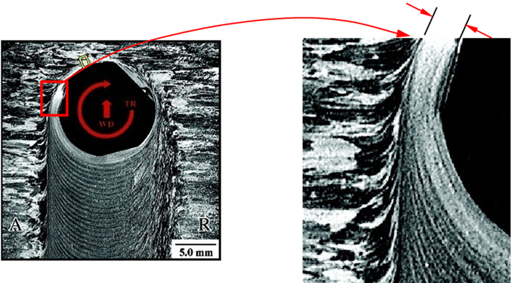
a FSW top cross-section;¹³ b shear band definition

A two-dimensional fully coupled thermal fluid model by Seidel and Reynolds¹⁰ considered lamina viscous and non-Newtonian flow around an ideal cylinder. Their results suggested that material transport occurs mainly around the pin on the retreating side. Similarly, Colegrove and Shercliff¹¹ used commercial fluid dynamics software and simulated coupled heat conduction and fluid flow effect FSW of 7075 Al alloy. A review summary on various modelling approaches is given by Nandan et al.¹²

Although a plenty of numerical models for FSW have been proposed or attempted over the last two decades, a modelling capability for process parameter window estimation¹ in terms of friction stir pin rotational and translational speed for a given material of interest remains elusive today. Recognising the dominance of local plastic deformation characteristics discussed in aforementioned work,^3–6 this paper presents a rather different approach to friction stir weld formation modelling by focusing on shear localisation process dynamics which should be directly applicable to the SB formation process shown in Fig. 1 as reported elsewhere.¹³ We start with a coupled thermal and visco-plastic formulation by idealising the shear formation process as a one-dimensional (1D) problem following the framework by Batra and Wei,¹⁴ but with different definitions of boundary and initial conditions that are directly relevant to FSW process.

Within this context, definitions of both time scale that governs the formation of an SB and length scale measuring SB width will be introduced. Together, these two parameters provide a theoretical estimate of the maximum SB propagation speed or maximum welding speed possible for a given material and a set of welding parameters. Friction stir welding experiments reported by Pilchak et al.⁷ and conducted in this study on FSW of Ti–6Al–4V alloy are then used to validate the theoretical estimates of maximum welding speeds observed in experiments. Finally, three drastically different metals are examined to gain insight on their friction stir weldability in terms of shear localisation parameters.

Note that material constitutive behaviour in this study is assumed to follow Johnson–Cook law in terms of dependency on temperature, strain and strain rate. One reason is that Johnson–Cook parameters for the materials of interest in this investigation have been well documented in a number of authoritative publications.^{15, 16} The other reason is that prior investigations into shear localisation instability in high strain rate thermal contact problems by Batra and Wei¹⁴ suggested the applicability of Johnson–Cook material model for modelling FSW processes Therefore, one additional objective of this investigation is to examine if Johnson–Cook material model is adequate in describing material behaviour in the strain rate and temperature regime that are relevant to friction stir weld formation process.

Shear localisation model

Model definition

As shown in Fig. 1b, a localised SB just formed neighbouring stir spin can be clearly identified with its width representing the tool advance for each tool revolution. The nearby material remains essentially stationary beyond a small distance from the SB boundary. At a peak strain rate of order of 10²–10⁴ s⁻¹ at SB surface in contact with stir pin, the associated heat transport process resulted from friction and plastic dissipation to its surrounding material can be reasonably assumed negligible, i.e. adiabatic.

As a result, relevant shear localisation problems can be further simplified as a thermal boundary layer problem (see Fig. 2) within which plastic deformation boundary layer is fully contained. Then, a governing characteristic length dimension (H) for such a thermal boundary problem can be treated as 1D transient heat conduction problem in the same way as illustrated in Fig. 2.

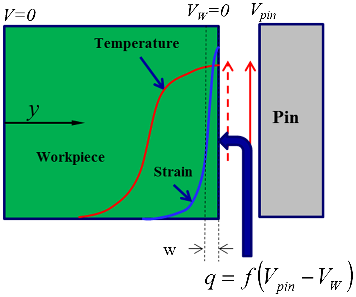
Definition of thermal boundary layer and plastic deformation boundary layer based shear localization problems

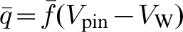
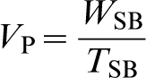
In Fig. 2, stir pin rotates at a constant speed V_pin while exerting a shear stress in contact with the workpiece (or base metal), where is frictional stress determined by applied torque. The resulting frictional heat flux generation 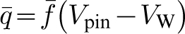is assumed to be fully consumed by the workpiece for simplicity. As the frictional heat builds up at base metal near stir pin surface, material softening occurs, resulting in rapid development of plastic straining at the base metal and stir pin interface. It should be pointed out that this modelling approach can be interpreted as taking a snap shot of SB formation process in time (within a time period of one revolution of the pin) and space (as described by the boundary layer problem in Fig. 2). As such, simulation terminates as soon as the relative velocity, i.e. V_pin−V_W approaches zero, i.e. sticking condition, or at the end of one revolution of the pin, depends on which comes first. After that a fully developed SB is realised. At this point, the corresponding SB width denoted as W_SB and the time elapse denoted as T_SB. Then, the corresponding SB propagation speed becomes (1) which can be interpreted as the theoretically maximum possible (or the optimum) welding speed we set out to investigate as one of the important FSW process parameters.

Governing equations

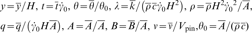
Consider a physical domain that occupies , which is subjected to applied frictional stress and a friction induced heat flux at the material/pin interface . Let the spatial coordinate ( ) be normalised by H, the shear stress by , time by H/V_pin and temperature by θ₀, where θ₀ is material reference temperature. In terms of non-dimensional variables, the domain now occupies the region bounded by planes with y = 0 and y = 1. Initially, the material behaves elastically with a rising temperature caused by frictional heating and associated conduction transfer. However, as yield strength of material decreases with increasing temperature, plastic deformation begins to develop. The governing equations for the thermal visco elastic– plastic problem can be written as follows (2) (3) (4) (5) (6)

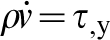
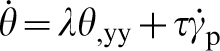
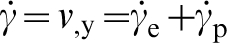
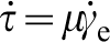
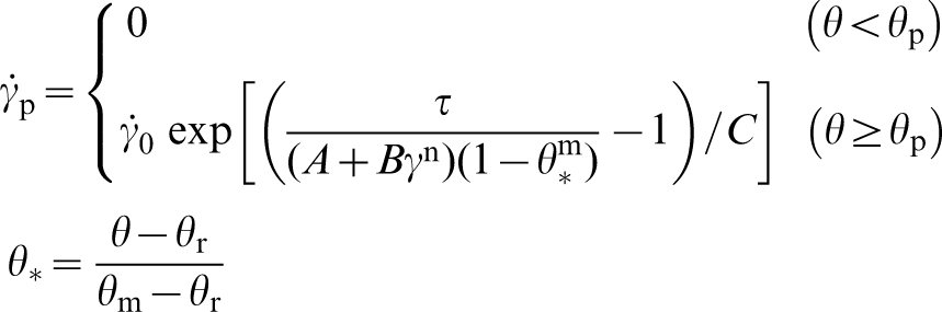
Here a superimposed dot signifies the time derivative; a comma followed by y indicates the partial differentiation with respect to y. In above equations, ρ is the mass density, v the velocity, τ the shear stress, θ the temperature, γ the shear strain which is partitioned into elastic part γ_e and plastic part γ_p. Furthermore, μ is the shear modulus and λ the thermal diffusivity of material. Equation (2) expresses momentum balance. Equation (3) is energy balance, in which plastic dissipation energy, represented by the second term on the right hand side, is assumed to be completely converted into heating. Equations (4) and (5) imply, respectively, the definition of strain rate and the Hooke's law written in rate form. Equation (6)¹⁶ is the constitutive equation of elasto-thermo-viscoplastic relationship, where θ_p is the temperature at which material yield strength equals to applied stress and θ_r, θ_m are room temperature and material melting temperature, respectively. All other material parameters are assumed to be independent of temperature.

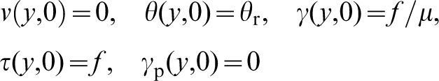
Note that the above formulations are introduced to simulate one single SB formation event corresponding to one revolution of pin rotation out of a continuous process of weld formation through shear localisation process. Therefore, the applied shear stress (f) on the boundary layer defined in Fig. 2 at t = 0 should be τ = f by definition due to equilibrium consideration. However due to adiabatic assumption for each individual shear localisation event, initial temperature at t = 0 within the boundary layer domain can be assumed to be room temperature. Then, at t = 0, initial conditions can be described as follows (7)

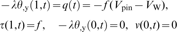
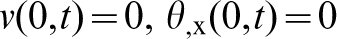
The corresponding boundary conditions are (8) which state that at the workpiece/pin interface, heat flux is induced by friction heating in the form of the product of applied frictional stress and relative velocity while at the other end of the domain (i.e. y = 0), can be realised as long as H is sufficiently large.

The non-dimensional parameters are related to their dimensional (barred) counterparts as follows (9) where is specific heat, thermal conductivity, and nominal strain rate. All are written in consistent dimensionless forms.

Numerical implementation

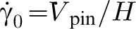
The shear localisation problem described by equations (2)–(9) can be conveniently solved numerically by means of a finite element method. In this investigation, the finite element implementation is through the use of the technical computing language supported by MATLAB.¹⁷ A MATLAB parametric programming code was developed using a weak form of the governing equations (equations (2)–(6)), initial conditions and boundary conditions (equations (7) and (8)) derived by a simple piecewise nonlinear Galerking/Petrov–Galerkin method. This discretisation method offers a good accuracy to the second order in space.¹⁸ The result is a system of coupled non-linear ordinary differential equations that can be integrated using MATLAB function ‘ode15s’. An adaptive time increment method is used to compute incremental solution over time within a prescribed accuracy requirement using built-in default tolerance settings, i.e. ‘Reltol’ = 10⁻³, ‘Abstol’ = 10⁻⁶, where Reltol and Abstol control the relative and absolute tolerances, respectively. The resulting MATLAB program developed can be used to obtain a full solution over time from t = 0 to a time at which material at workpiece/pin interface reaches to a prescribed pin surface linear velocity, i.e. v (1,t) = 1, at which time an SB of width W_SB in equation (1) is considered to be fully developed and the simulation terminates.

The coordinates of finite element model grid (i.e. nodal positions) is given by (10) with equation (10), a finer resolution is attained at material/pin interface (i.e. y = 1) where applied shear stress and heat flux are prescribed.

Modelling of welding experiments

In this section, the modelling procedures described above are used to simulate a set of selected FSW experiments reported by Pilchak et al.⁷ and conducted as a part of this study. Along with the discussions of experimental results, the definitions of shear localisation parameters described in equation (1) will be illustrated in detail.

Data by Pilchak et al.⁷

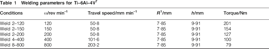
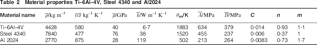
A total of five mill-annealed Ti–6Al–4V friction stir welded specimens (see Table 1) were produced with good weld quality by using a range of welding parameters through prior experiences.⁷ Table 1 shows welding parameters used in Ref. 7. The Johnson–Cook material constants are summarised in Table 2, taken directly from a Federal Aviation Administration report.¹⁵

Table 1

Welding parameters for Ti–6Al–4V⁷

Conditions	ω/rev min^–1	Travel speed/mm min^–1	R¹/mm	h/mm	Torque/Nm
Weld 2–120	120	50·8	7·85	9·91	201
Weld 2–150	150	50·8	7·85	9·91	154
Weld 2–200	200	50·8	7·85	9·91	127
Weld 4–400	400	101·6	7·85	9·91	100
Weld 8–800	800	203·2	7·85	9·91	79

Table 2

Material properties Ti–6Al–4V, Steel 4340 and Al2024

Material name	/kg m^–3	/J kg^–1 K^–1	/GPa	/W m^–1 K^–1	θ_m/K	/MPa	/MPa	C	n	m
Ti–6Al–4V	4428	580	40	6·7	1883	634	379	0·014	0·93	1·1
Steel 4340	7840	477	76	38	1520	455	237	0·006	0·37	1
Al 2024	2770	875	28	119	502	213	264	0·0083	0·73	1·7

In applying the shear localisation model described in the section on ‘Shear localisation model’ of this paper, we only need to investigate shear localisation within a time period of one revolution of stir pin in order to extract SB width and time required. As such, a time domain of interest becomes t_c = 1/ω, where ω is the angular velocity of pin rotation (revolution s^–1). A spatial domain H in Fig. 2 can be defined as H = 5H_c where 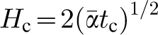is a characteristic length in thermal diffusion process and is thermal diffusivity of material. As to be shown in the next section, with H = 5H_c, an one-dimensional semi-infinite body condition is realised in Fig. 2. Frictional stress is estimated by the applied torque and stir pin geometric parameters used in these welding experiments, as summarised in Table 1, i.e. 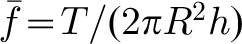, where T is the applied torque, R is the radius of the pin and h is the height of the pin.

Modelling results

For illustration purpose, modelling results corresponding to conditions under ‘Weld 2–120’ (see Table 1) are shown in Fig. 3. Note that predicted temperature (Fig. 3a) is normalised by material melting temperature and material flow velocity by stir pin velocity V_pin. In order to examine detailed transitional behaviour from elastically dominated deformation to plastic deformation, the vertical axes in Fig. 3b–d, are presented in logarithmic scale. Note that the analysis terminates when the relative velocity at the interface between base material and stir pin becomes zero, i.e.

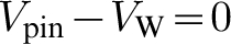
a temperature; b plastic strain rate; c plastic strain; d velocity

Figure 3a shows predicted special temperature distributions within base metal at different times in seconds. The material/pin interface temperature is relative low at the beginning (e.g. t≈0·11 s) and continue to increase over time. Before time reaches to about t≈1·06 s, temperature throughout the domain remains relatively low and the resulting plastic deformation is still barely noticeable (see Fig. 3b–c). The same can be said about material flow velocity, see Fig. 3d. As the interface temperature (y = 0) rapidly increases due to continued friction heating, thermal softening term in Johnson–Cook model (equation (6)) begins to take effect. As time reaches to t≈1·06 s and beyond, a localised development of plastic strain rate and plastic strain can be clearly seen near material/pin interface (i.e. y = 0). Material at and near the interface starts to accelerate, resulting in a rapid increase in velocity, as shown in Fig. 3d. Even though the temperature exhibits only a slight increase during t≈1·06–1·28 s, plastic strain, plastic strain rate, and interface material velocity increase rapidly. With the presence of high temperature gradient near the interface, e.g. y>0·95, both spatial plastic strain, plastic strain rate, and velocity distributions become increasingly localised, forming two distinct zones in space after t≥1·2 s, as shown in Fig. 3b–c. A demarcation position separating the two zones in space occurs at y≈0·985 from material/pin interface at t = 1·28 s, which can be seen in all three parameters predicted, i.e. plastic strain, strain rate, and velocity, suggesting the onset of SB development within the small region of y≈0·985∼1, often referred to as shear localisation in continuous mechanics terms.

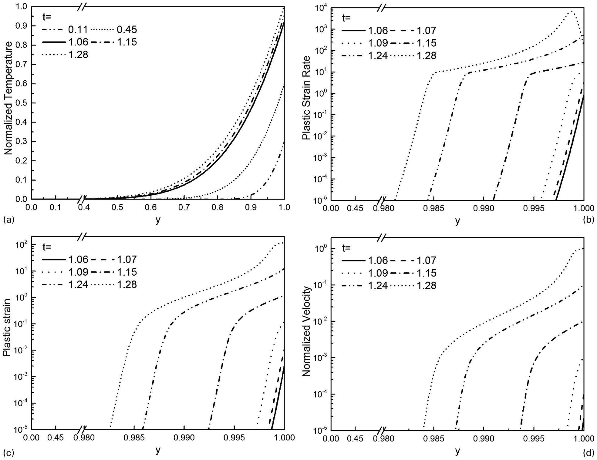
In order to verify the generality of the shear localisation phenomena observed for conditions corresponding to ‘Weld 2–120’ in Table 1, the modelling results for all five weld samples and associated welding conditions reported by Pilchak et al.⁷ are compared in Fig. 4. Although with rather similar spatial temperature distributions (Fig. 4a), the predicted plastic strain, strain rate, and velocity distributions show significant differences among the five sets of welding conditions (see Fig. 4b–d). However, a clearly defined deflection point can be identified in spatial distribution behaviour, which moves increasingly closer to the interface from y≈0·985 to y≈0·995, as pin rotation speed increases from 120 (Weld 2–120) to 800 rev min^–1 (Weld 8–800). Beyond the deflection point (or a further increase in y), plastic strain, plastic strain rate, and velocity exhibit similar distribution characteristics among all five cases, similar to the finding discussed earlier with respect to the case for ‘Weld 2–120’. Given the results obtained so far shown in Figs. 3 and 4, it can be concluded with a reasonable degree of confidence that SB localisation phenomena associated with friction stir weld formation process are adequately captured with the shear localisation model presented in the previous section. We can then proceed to estimate theoretical welding speed for each of the five cases by extracting SB width W_SB and SB formation time T_SB in equation (1).

a temperature; b plastic strain rate; c plastic strain; d velocity

Before proceeding, it is worth noting that the temperature distributions in Fig. 4a, show rather small spatial variation over the five sets of welding parameters, all of which reaches to the melting temperature (i.e. with normalised temperature being unity) at workpiece/pin interface. A careful examination of the modelling results associated with this phenomenon and the theoretical formulation in equation (6) suggests that this is solely due to the structure of John–Cook model. When the workpiece material at the interface rises to the pin rotational speed, the high plastic strain renders the strain hardening term so dominant that the resulting high yield stress accelerates friction heating at the interface until the interface temperature reaches to its melting point. This also points out one limitation of Johnson–Cook model for modelling FSW, which inevitably predicts melting temperature at the interface under typical welding conditions. In light of this finding, an alternative constitute model such as Zener Hollowman type has been shown to be more appropriate for modelling FSW¹⁹ in a follow on study, when it was incorporated for analysing the same set of experimental data.

Shear band width

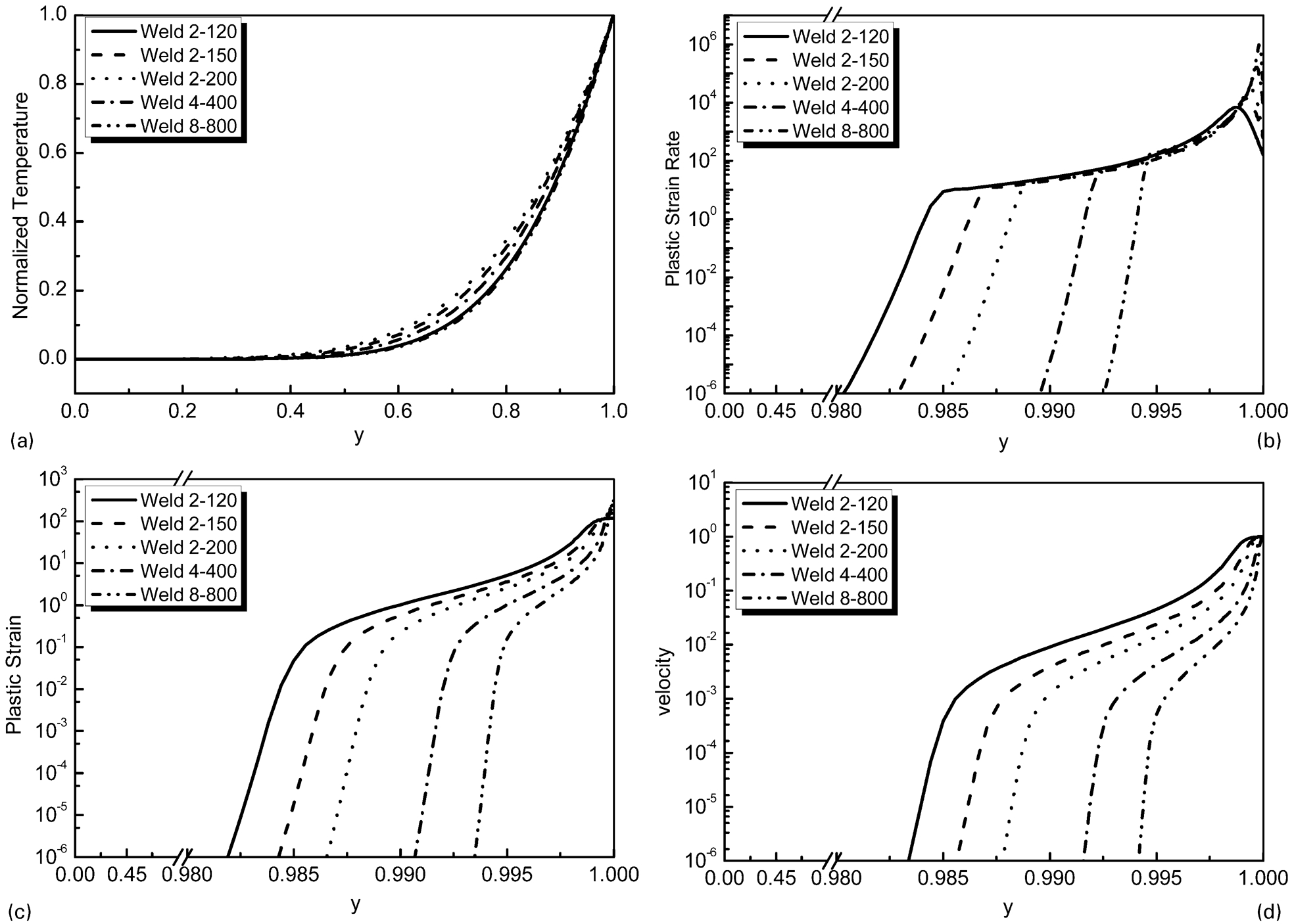
Figure 5 is a re-plot of the plastic strain, strain rate, and velocity fields in Fig. 3 by focusing attention in the region containing SB development. All three predicted field parameters (plastic strain, strain rate, and velocity) indicate an essentially same demarcation position in y, beyond which a distinct change in rate over spatial coordinate (y) can be clearly seen. The region from y≈0·985 to material/pin interface, i.e.y = 1 can be defined the SB width. Since y is normalised by H = 5H_c, the actual SB width becomes (1–0·985)×5H_c, yielding an SB width of 0·18 mm. Figure 6 shows a banded structure of a friction stir welded Ti–6Al–4V sample produced in this study, which shows a width of 0·23 mm. The comparison in terms of SB widths can be considered as being acceptable, given the simplicity of the 1D model (Fig. 2), temperature independent thermal–physical properties in equation (6), and uncertainties involved in the material constitutive model.

Log plot of spatial distributions of velocity, plastic strain, and plastic strain rate distribution for Weld ID 2–120

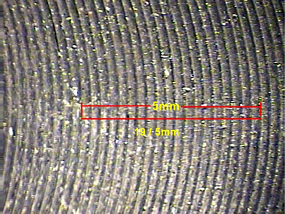
Banded structure of friction stir welded Ti–6Al–4V sample, showing band width about 0·23 mm

Shear band formation time

By considering the case for ‘Weld 2–120’ in Table 1, without losing generality, Fig. 7 shows time–history plots of normalised temperature, plastic strain rate, plastic strain, and velocity for material point at the material/pin interface, i.e. at y = 1. In logarithmic scale, plastic strain rate as a function of time shows a sudden change in its time rate at t = 1085 s, which can also been observed in plastic strain and velocity histories (see Fig. 7c and d). This deflection point in time signifies the initiation of SB. The time duration accumulated from this point to the completion of one full revolution of stir pin rotation (i.e. V_pin−V_W = 0) defines the SB formation time, T_SB. Furthermore, it is worth noting that after initiation, plastic strain and velocity histories continue to show a monotonic rise, although with a slower rate, plastic strain rate history at first increases rapidly and then show a drastic drop from its peak. Again, this phenomenon is unique to Johnson–Cook law in which plastic strain rate is governed by both thermal softening and strain hardening terms γⁿ where m and n are thermal softening and strain hardening exponents, respectively. Before reaching its peak, plastic strain remains nearly zero until temperature increases to about 0·9T_m or 90% of material melting temperature. Prior to reaching to this point, the strain hardening term dominates the strain rate development as a function of time. When temperature reaches to a neighbourhood around θ≈0·9T_m, thermal softening term starts to drive a rapid increase in plastic strain rate resulted from a rapid decrease in shear strength under applied constant shear traction stress. This leads to an explosive increase in plastic strain (Fig. 7c), which in turn increases shear strength, enabling the dominance of the strain hardening term again, resulting in a rapid decrease in plastic strain rate.

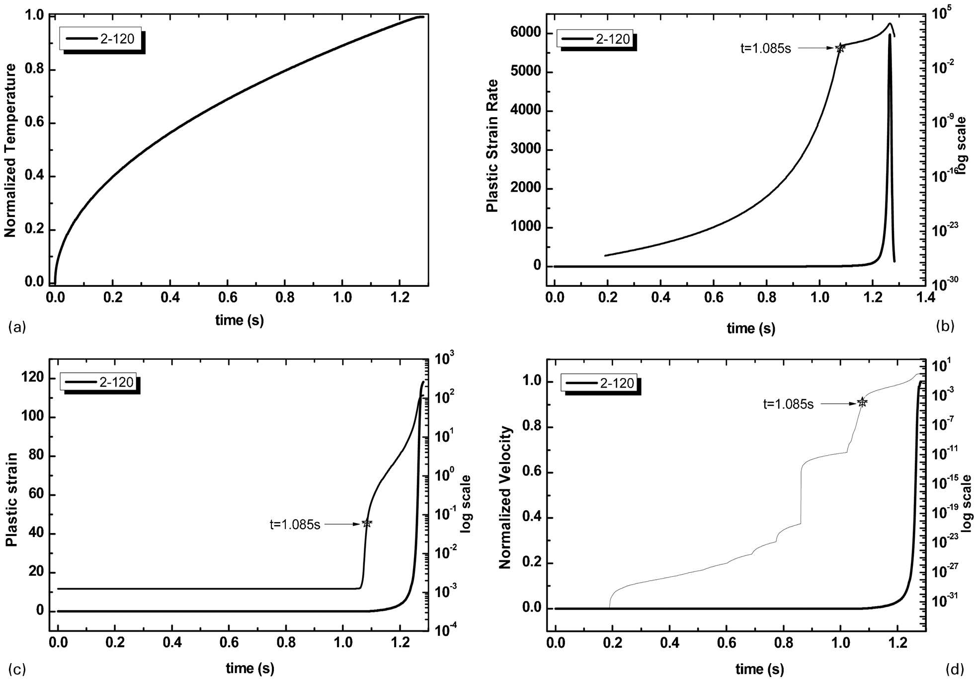
a normalised temperature rise; b plastic strain rate; c shear strain; d velocity

Welding speed estimation

Since both SB width and its formation time have been already defined in the previous sections, SB propagation speed, which is the maximum possible welding speed in FSW, can then be calculated through equation (1). The modelling results are summarised in Fig. 8a and b for the five welding conditions in Table 1. The predicted maximum possible welding speeds are compared with actual welding speeds used in FSW experiments in Fig. 8c. It can be seen that both SB width and formation time decrease with an increasing rotational speed. It is important to note that SB formation time decreases in a faster rate than SB width as a function of pin rotation speed, leading to a faster SB propagation speed or welding speed while maintaining a consistent weld quality. The theoretically estimated maximum welding speeds for all five welding conditions compare well with experimental findings from Pilchak et al.,⁷ in which welding parameters used to achieve acceptable weld quality were obtained experimentally (Fig. 8c). The predicted maximum welding speed is somewhat higher than that used in experiments, which seems reasonable since the calculation result is ‘maximum welding speed’, while the weld speed used in experiment is decided through trials and may not be the optimum value.

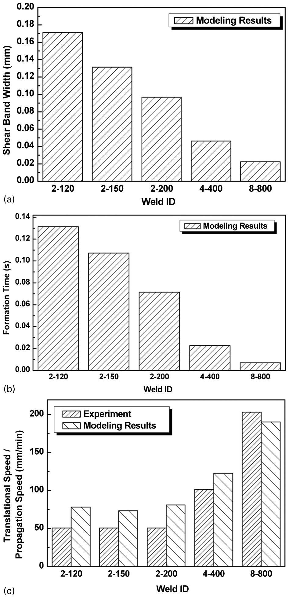
a shear band width; b shear band initiation time; c shear band propagation speed and comparison with pin translational speed given from experiment

Discussion

As shown in the section on ‘Welding speed estimation’, the shear localisation modelling procedure developed here provides reasonable estimates of SB width, SB formation time, and theoretical maximum welding speed. In this section, the application of the present modelling are used to study different base material effect, i.e. Ti–6Al–4V, Steel 4340, Al2024. Then the issue caused by Johnson–Cook constitutive law is discussed.

Material effects

Thus far, the analysis has been focused upon titanium alloy Ti–6Al–4V. It should be informative to examine some of the fundamental differences in shear localisation process among the three rather different materials, such as titanium versus steel versus aluminium. In doing so, two more materials are considered here: high strength low-alloy steel 4340 and high strength aluminium alloys Al 2024 on which Johnson–Cook model properties are also available from,^{15, 16} as given in Table 2. In addition, yield strength as a function of temperature for each material is also given in Fig. 9.

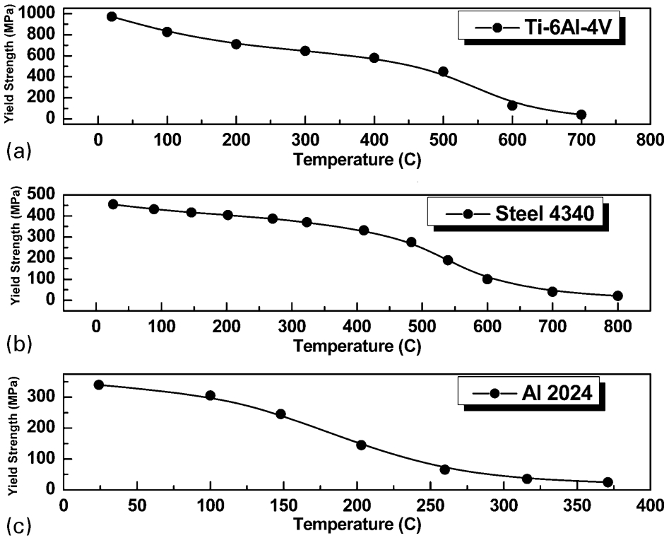
Yield strength as function of temperature of a Ti–6Al–4V, b Steel 4340 and c Al2024

For easy comparison purpose, all calculations for the three materials are performed under the same frictional stress (f = 60 MPa) and same rotational speed (500 rev min^–1), and same flux (1·571×10⁷ W m^–2). The results are summarised in Fig. 10. In Table 2, , and n characterise material's strain hardening ability. It can be seen that Ti–6Al–4V shows the strongest strain hardening term among the three materials and Al2024 shows the weakest strain hardening term. The strain hardening ability symbolises material's resistance to SB formation. A material possesses a higher strain hardening ability would require a higher temperature to be reached in order for its thermal softening term to overcome plastic deformation resistance. Under the same friction heat input conditions, a material with a lower strain hardening ability requires a lower temperature to overcome its plastic deformation resistance, resulting in a wider SB. This is consistent with the results shown in Fig. 10b. The high strain hardening term and low thermal conductivity of Ti–6Al–4V result in rather localised SB characterised by small width and short formation time. For Al2024, its low strain hardening ability and high thermal conductivity promotes the formation of a wider SB within a relatively short period time.

a plastic temperature; b shear band width; c shear band formation time; d shear band propagation speed

As for Steel4340, its strain hardening ability is not as strong as Ti–6Al–4V while its thermal conductivity is nearly 6 times higher than Ti–6Al–4V. As a result, 4340 tends to form a wider SB within a longer period formation time, leading to somewhat a slower welding speed than Ti–6Al–4V. In summary, the predicted maximum welding speed is the highest for Al2024 among all three materials studied here. Interestingly enough, both Steel 4340 and Ti–6Al–4V are rather similar in maximum welding speeds, with Steel 4340 being slightly lower. However, the narrowest SB width predicted for Ti–6Al–4V suggests that Ti–6Al–4V should possess the poorest FSW weldability, i.e. sensitive to pin translational speed. The widest SB width predicted for Al2024 is consistent with the fact that aluminium alloys often possess a good FSW weldability.

About Johnson–Cook model

Although all calculation results using Johnson–Cook material model seem reasonable as far as shear localisation parameters are concerned, this work has identified one area that requires further investigation regarding its suitability for modelling FSW process. This is illustrated in Fig. 4a. In this figure, material at the interface for all five cases reaches melting temperature under different rotation and translational speeds, which is considered unlikely. This is because Johnson–Cook¹⁶ determined material parameters from torsional test data over a (relative low) range of strain, strain rate and temperature. The strain hardening term in Johnson–Cook model is expressed as A+Bγⁿ, and the relationship between plastic strain and strain hardening term is plotted in Fig. 11. It can be seen that when plastic strain reaches to 100–200, which is usually the case when dealing with FSW, the resulting hardening effects generate a yield stress to a value that is about 40 to 80 times higher than room temperature value. This suggests that Johnson–Cook model is a strain hardening dominated material model. As such, thermal softening term does not play a significant role until material temperature reaches near melting temperature, i.e. not suited for high temperature material behaviour characterisation in a temperature regime below melting. Typical hot forming (e.g. forging, extrusion, etc.) takes advantage of thermal softening effects which are dominant at a desirable forming temperature. A great deal of evidence generated in hot forming research community show that material at such a temperature possesses little strain hardening ability if at all.²⁰ Furthermore, some indirect temperature measurements performed by Pilchak et al.⁷ suggests that the five welding conditions in Table 1 resulted in different interface temperatures which should be below material melting temperatures. For above reasons, an alternative constitutive material model will be examined in a subsequent paper¹⁹ by the same authors, which clearly show more reasonable results than Johnson–Cook model.

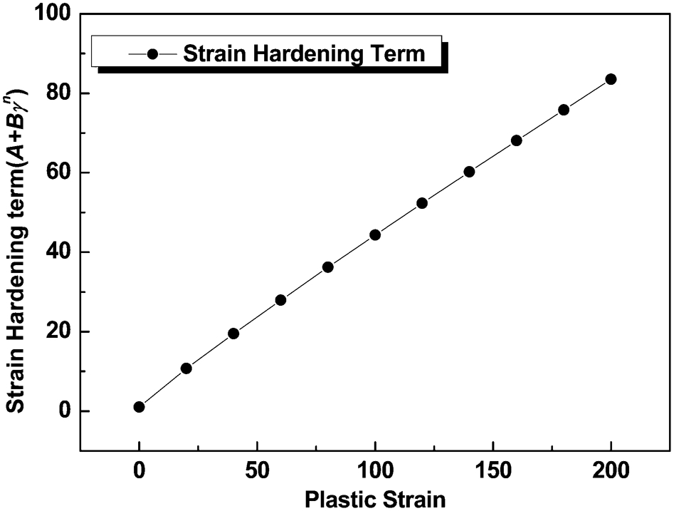
Dependency of strain hardening term

Summary

A shear localisation model is presented in this paper, which focuses on SB formation phenomena associated with FSW process. With this model, SB width, SB formation time, and SB propagation speed can be theoretically estimated. The SB propagation speed serves a direct estimate of the maximum welding speed possible for a given material to be welded under a set of specified stir pin rotational and translational speeds. The model is shown to provide reasonable estimations of shear localisation parameters against recent experimental data on titanium alloy Ti–6Al–4V.

By considering three drastically different base materials, predicted shear localisation parameters clearly indicate that titanium alloy such as Ti–6Al–4V is most difficult to weld due to its narrowest SB width among all three materials considered. Even though Steel 4340 exhibits a slightly lower welding speed Ti–6Al–4V, its significantly wider SB width suggests a much better friction stir weldability than Ti–6Al–4V. Aluminium alloys such as Al 2024 possesses the best friction stir weldability among the three materials examined, because of its widest SB width and a modest amount of time needed for SB formation.

Footnotes

Acknowledgements

The authors acknowledge the support of this work in part by ONR Grant No. N00014-10-1-0479 at UNO and the National Research Foundation of Korea (NRF) Gant funded by the Korea government (MEST) through GCRC-SOP at University of Michigan under Project 2-1: Reliability and Strength Assessment of Core Parts and Material System.

References

Dawes

and Thomas

: ‘Friction stir joining of aluminum alloys’, TWI Bulletin (6), Cambridge, UK, November/December 1995.

Nandan

, DebRoy

and Bhadeshia

HKDH

: ‘Recent advances in friction stir welding – process, weldment structure and properties’, Prog. Mater. Sci., 2008, 53, 980–1023

Nunes

: ‘Prolegomena to the study of friction stir welding’, Proc. Materials Science & Technology 2010 – Joining of Advanced and Specialty Materials XII, Houston, TX, USA, October 2010, Paper 14, pp. 2651–2664.

Schneider

and Nunes

Jr : ‘Characterization of plastic flow and resulting microtextures in a friction stir weld’, Metall. Mater. Trans. B, 2004, 35B, (4), 777–783

Yang

, Yan

, Sutton

and Reynolds

: ‘Banded microstructure in AA2024-T351 and AA2524-T351 aluminum friction stir welds, Part I. metallurgical studies’, Mater. Sci. Eng. A-Struct., 2004, A364, 55–65

Knipling

and Fonda

: ‘Texture development in the stir zone of near-a titanium friction stir welds’, Scr. Mater., 2009, 60, 1097–1100

Pilchak

, Tang

, Sahiner

, Reynolds

and Williams

: ‘Microstructure evolution during friction stir welding of mill-annealed Ti-6Al-4V’, Metall. Mater. Trans. A, 2011, 42A, (3), 745–762.

Dong

, Lu

, Hong

and Cao

: ‘Coupled thermomechanical analysis of friction-stir welding process using simplified models’, Sci. Technol. Weld. Join., 2001, 6, (5), 281–287.

Schmidt

, Hattel

and Wert

: ‘An analytical model for the heat generation in friction stir welding’, Model. Simul. Mater. Sci., 2004, 12, (1), 143–157.

10.

Seidel

and Reynolds

: ‘Two-dimensional friction stir welding process model based on fluid mechanics’, Sci. Technol. Weld. Join., 2003, 8, (3), 175–183.

11.

Colegrove

and Shercliff

: ‘3-Dimensional CFD modelling of flow round a threaded friction stir welding tool profile’, J. Mater. Process. Technol., 2005, 169, (2), 320–327.

12.

Nandan

, Roy

and DebRoy

: ‘Numerical simulation of three-dimensional heat transfer and plastic flow during friction stir welding’, Metal. Mater. Trans. A, 2006, 37A, (4), 1247–1259

13.

Fonda

, Bingert

and Colligan

: ‘Development of grain structure during friction stir welding’, Scr. Mater., 2004, 51, (3), 243–248.

14.

Batra

and Wei

: ‘Shear bands due to heat flux prescribed at boundaries’, Int. J. Plast., 2006, 22, (1), 1–15.

15.

Federal Aviation Administration (FAA) Office of Aviation Research Report, ‘Experimental investigations of material models for Ti-6Al-4V titanium and 2024-T3 aluminum’, Washington, D.C. USA, 20591.

16.

Johnson

and Cook

: ‘A constitutive model and data for metals subjected to large strains, high strain rates and high temperatures’, Proc. 7th Int. Symp. on ‘Ballistics’, Vol. 21; 1983, The Hague, International Ballistics Committee.

17.

MATLAB User's Guide, The MathWorks, Inc. Natick, MA, USA, 1998.

18.

Skeel

and Berzins

: ‘A method for the spatial discretization of parabolic equations in one space variable’, SIAM J. Sci. Stat. Comp., 1990, 11, (1), 1–32.

19.

Pei

and Dong

: ‘Modeling of shear band formation process in friction stir welding’, submitted for publication in Journal of Materials Processing Technology, March 2014.

20.

McQueen

and Ryan

: ‘Constitutive analysis in hot working’, Mater. Sci. Eng. A, 2002, A322, (1), 43–63.