
Abstract
The change in temperature distribution due to constriction of an electric current through a contact area is analytically and numerically investigated. The potential distribution, current density distribution and heat density distribution inside the body are analytically obtained. The heat density has the singular point at the periphery of the contact area. It is revealed that the temperature has a finite value at the periphery, whereas the temperature change rate with respect to time has an infinite value because of the singularity. The results show the change in the temperature distribution. The times to melting and melting area are determined from the change in the temperature distribution. The total heat generated until melting occurs is also obtained.
Keywords
Introduction
Heat generation by constriction of an electric current through a contact area as shown in Fig. 1 is important for technological applications such as resistance spot welding, electric relays, and electric and electronic switches. The heat changes the conditions in the contact area, and knowledge of the conditions is important for device design.
It is apparently difficult to observe the contact area directly. The conditions in the contact area are checked using relevant methods such as measuring the electric resistance or electric current.1–5 To understand the conditions in the contact area, it is important to understand the relation between changes in the conditions and the changes in the electric resistance or electric current. Real surfaces have surface roughness, and the actual contact areas are tiny.6–8 The electric current flows through these tiny spots, and the heat generated by constriction of the current softens or melts the contact area. The contact area deforms, and its conditions change. Thus, heat generation around the tiny contact area is of primary importance. We focus on a single tiny spot for simplicity.
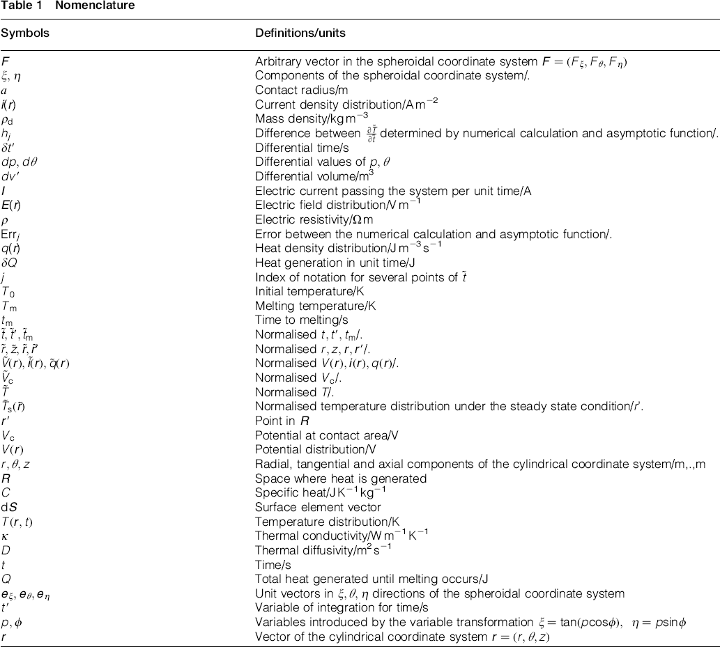
Nomenclature
The current density distribution inside the body was analytically obtained by Greenwood and Williamson under the steady state condition, in which the temperature distribution does not change. 9 The theory is a development of the research of Kohlrausch, who obtained the relation between the temperature and potential inside the body under the steady state condition. 10 The heat density distribution is derived from the current density distribution, and the heat density has a singular point at the periphery of the contact area. In contrast, the temperature distribution under the steady state condition, which was also obtained by Greenwood and Williamson, does not have a singular point and has the same value at the contact area.
Experiments show that melting occurs around the periphery of the contact area.9, 11 From the analysis by Greenwood and Williamson, melting occurs before the temperature distribution reaches the steady state. Kohler and Zielasek analytically derived the temperature change, but they focused only on the temperature change at the centre of the contact area and did not discuss the change in the temperature distribution in other regions, including the periphery of the contact area. 12
The change in the temperature distribution, including that at the periphery of the contact area, has been numerically analysed using the finite element method. However, the calculation around the singular point of the heat density distribution is not clear. Kubono removes the effect of heat generation at the point, 13 and Robertson does not clearly mention how to treat that point. 14
This research analytically and numerically investigates the change in the temperature distribution due to constriction of an electric current through the contact area. We first introduce a simple system for the analysis. Then, the change in the temperature distribution is derived. The singularity is strictly discussed. The results suggest the time to melting, melting area and total heat generated until melting occurs, which corresponds to the total energy consumption until melting occurs. Those results facilitate understanding of the change in the condition of the contact area and theoretical research on applications such as resistance spot welding.15–17 1
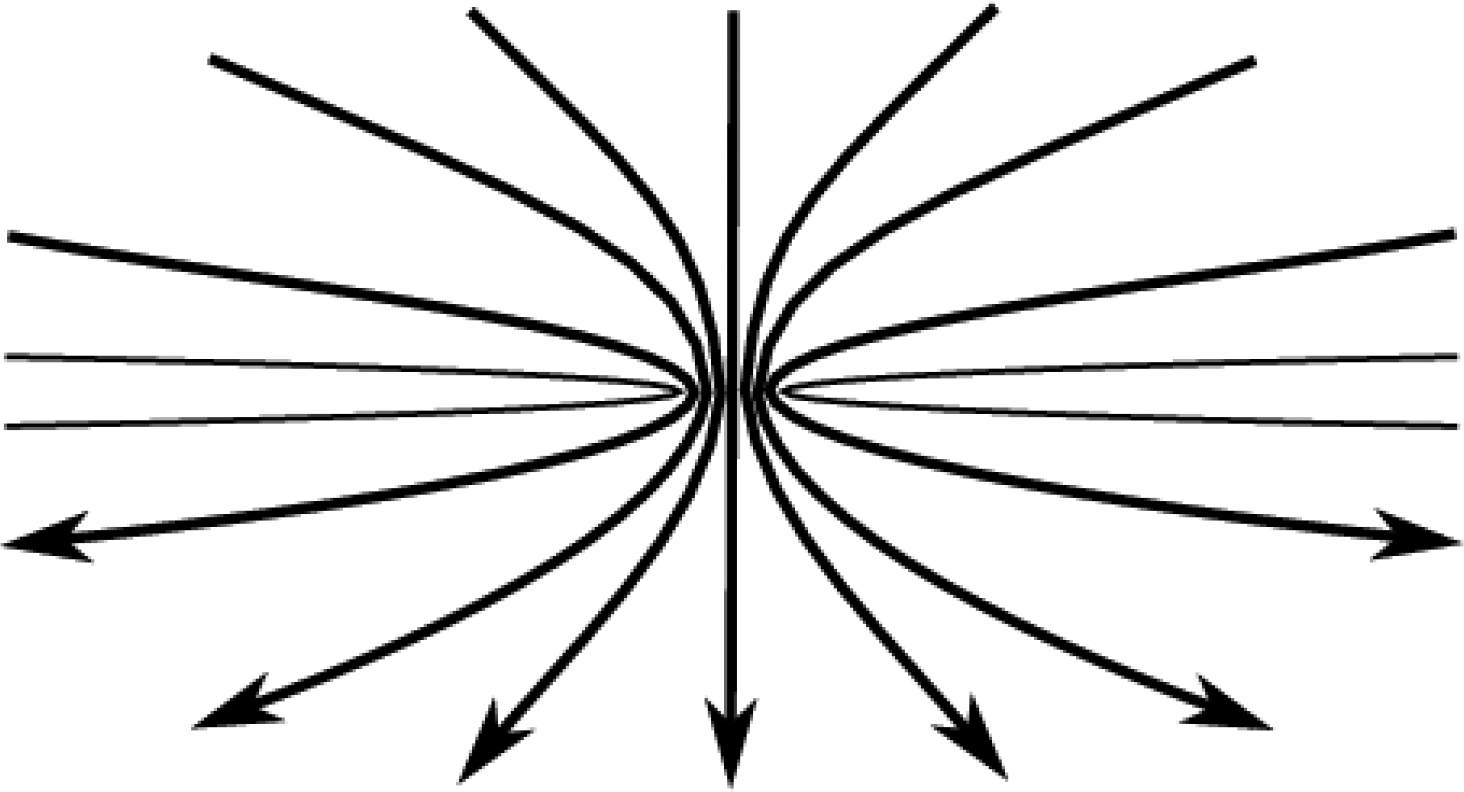
Schematic illustration of constriction of electric current through contact area
Theory
System
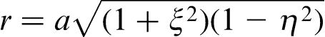
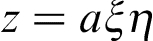
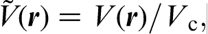
Figure 2 shows the axially symmetric semi-infinite conductive system introduced in this research. The shaded area represents the contact area, and a is the contact radius (m). Regarding the coordinates, the origin O is set at the centre of the contact area, the axis of symmetry is the z axis, the radial direction is the r axis, and the direction tangential to the circle is the θ axis. An arbitrary point inside the body is expressed as
 . Regarding the boundary conditions, at the contact area
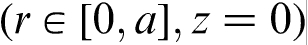 , the potential is Vc (V); at an infinite distance from the contact area, the potential equals zero; at the upper surface of the body excluding the contact area (r>a, z = 0), the component normal to the surface of the gradient of the potential equals zero.
Schematic illustration of system
Derivation of current density distribution
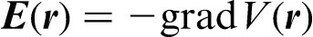
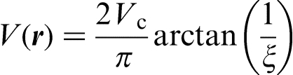
If the magnetic effect is ignored, the potential distribution V(
Consider V(
 and
and
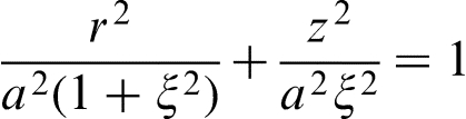
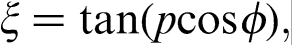
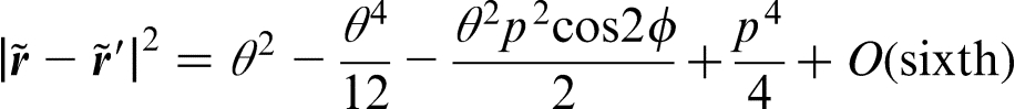
 . θ is the same for both coordinate systems. Equations (6a) and (6b) are transformed into equation (7) by eliminating η, where it is easier to understand that ξ, θ, η express the spheroid.
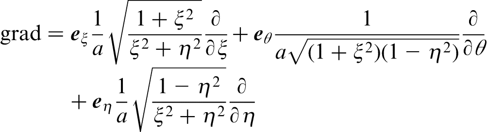
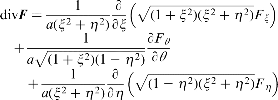
 are unit vectors in the directions. ξ, θ, η respectively and
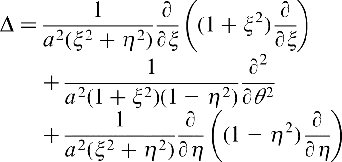
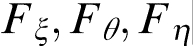 are the components of arbitrary vector F in the spheroidal coordinate system. From equations (8) and (9), the Laplace operator in the spheroidal coordinate system is derived as
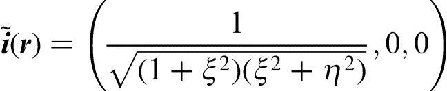
If we normalise
 as
as
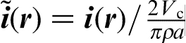 , then
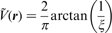
Derivation of temperature distribution change
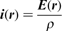
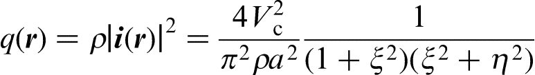
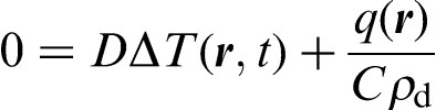
The heat density distribution q(
 , then
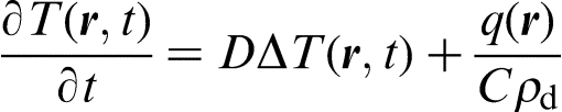
 is the thermal diffusivity (m2 s− 1), C is the specific heat (J K− 1 kg− 1), ρd is the mass density (kg m− 3), κ is the thermal conductivity (W m− 1 K− 1), and t is the time (s). We define t = 0 when Vc is applied to the contact area.
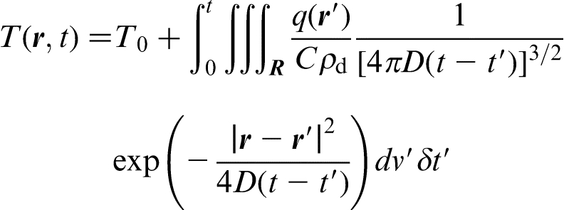
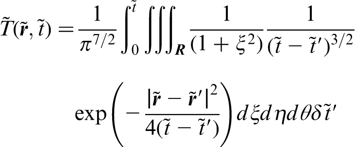
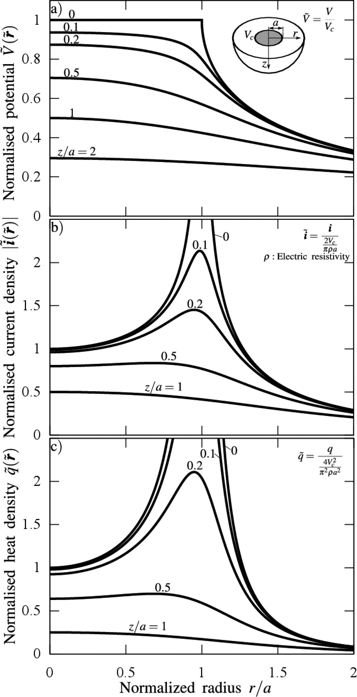
Assuming that the material constants (specific heat, mass density and thermal conductivity) are uniform and constant, and that the effects of the phase transition are ignored, the change in the temperature distribution for an arbitrary heat density distribution is obtained as follows by solving equation (16).
 ), and
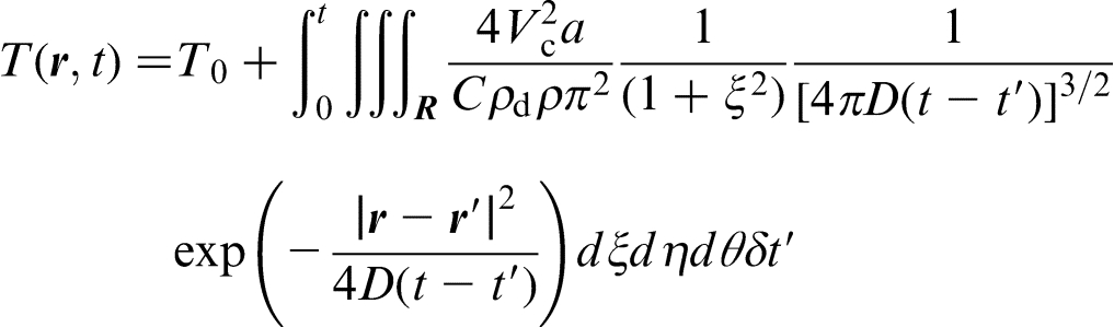
 is the differential of t′. From equations (14) and (17) and
 , the change in the temperature distribution for the constriction of the current is obtained as follows:
 (if
(if
 . Thus,
 ,
,
 and
and
 . The normalised temperature distribution change is then obtained as
 . The range of η is
 and is not
 because the upper surface of the body is assumed to be isothermal, and heat propagates as if it is reflected at the boundary.
The temperature distribution is axially symmetric. Thus,
 , and
, and
 .
.
Results and discussion
Results
Figure 3a–3c shows
 ,
,
 and
and
 respectively obtained using equations (12), 13 and (15). The gradient of the potential distribution with respect to the radius is discontinuous at the periphery of the contact area (
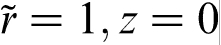 ). Thus, the current density distribution and heat density distribution have a singularity at the same point. The singularity causes an infinite temperature change rate with respect to time.
a normalised potential; b normalised current density; c normalised heat density
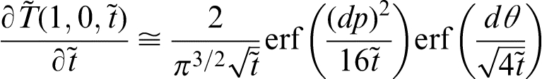
We differentiate equation (19) with respect to
 and obtain
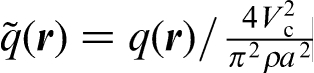
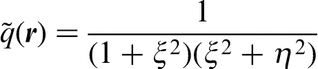
 is normalised as
 .
.
 has a finite value when
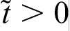 . When
 , the diffusion, which is the first term of equation (16), equals zero. Thus,
 has a singular point at
 . This singularity is derived from the singularity of the current density distribution.
The temperature change rate has an infinite value at the periphery of the contact area when
 . However, this does not mean that the temperature has an infinite value. Consider the heat diffusion from a point where heat is input. The heat diffuses just after it is input and is widely distributed in space. Thus, the heat diffuses into a wider region as the elapsed time since the heat input increases. Therefore, if the elapsed time is short, the heat is concentrated near the point where it is input. Next, consider the heat input distribution. The temperature change rate is determined by integrating the heat diffusion from all the points where heat is input. When the elapsed time since the heat input is long, it is necessary to integrate the heat diffusion from distant points. When the elapsed time is short, the temperature change rate is estimated by integrating only the heat diffusion from the vicinity.
The singular points are
 . It is sufficient to calculate the temperature change rate with respect to
 at
at
 because of the axial symmetry. Thus, we can approximately calculate equation (20) by integrating the heat diffusion around
 when
when
 . We set
 , where
 ; then,
 is expanded in a series as
 corresponds to
 . When
 , the integral range can be constricted as
 , where
 satisfy
 . If
. If
 , then
 is approximated as
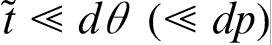 , the terms of the error function equal one. Thus,
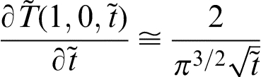
 . From equation (25),
 has an infinite value at
 ; however, the integration of
 with respect to
 is
is
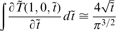
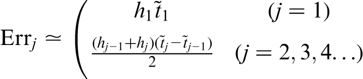
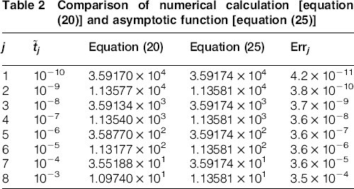
Table 1 compares the numerical calculation [equation (20)] with the asymptotic function [equation (25)] and shows the error arising from the introduction of the asymptotic curve. The index j represents several points of
 . Err
j
is defined as shown in Fig. 4 and is estimated as the area of the trapezoid formed by the intersection points of the two curves and the lines
. Err
j
is defined as shown in Fig. 4 and is estimated as the area of the trapezoid formed by the intersection points of the two curves and the lines
 and
and
 . Note that when j = 1,
 is approximated by a rectangle. Thus,
 .
.
Comparison of numerical calculation [equation (20)] and asymptotic function [equation (25)]


Error estimation of asymptotic curve near
The change in the temperature distribution at the upper surface (
 ) of the semi-infinite body is shown in Fig. 5a. The temperature increases as the region at the periphery of the contact area becomes larger. Then, the temperature around the centre of the contact area increases and takes almost the same value inside the contact area. Figure 5b shows the change in the temperature distribution inside the body. The temperature monotonically decreases with respect to
 . The temperature at
 decreases more gradually with respect to
 than at
 .
.
Change in normalised temperature
: a at upper surface for several
 , where horizontal axis is
 ; b inside body at
 for several
 , where horizontal axis is
 ; c at upper surface and inside body, where horizontal axis is
 ; range of
 in c is expanded to d
 ; in b–d, solid lines represent
 and dotted lines represent
Figure 5a and 5b shows that, when
 , the temperature distribution reaches the steady state, where the amount of heat diffusion and the amount of heat generation agree at each point, and the temperature distribution does not change. From equation (16), the condition is
 is obtained as
Figure 5c shows the temperature change at several points. When
 , the temperature increases at the periphery of the contact area. Then, for
 , the temperature at the centre of the contact area increases, taking almost the same value as at the periphery of the contact area around
 . Figure 5d shows the detailed temperature change for
 . After
 , the temperature almost reaches the steady state around
 .
.
Applications
We discuss the applications of the obtained results. Conventional experiments on the point contact current showed that the periphery of the contact area melted (see Fig. 5a).9, 11 The temperature obviously has different values at the periphery and the centre of the contact area for a while after the current begins to flow. The values become closer and have almost the same value at
 , as shown in Fig. 5c. The result suggests that the conventional experimental studies were done under the condition
 .
.
If the steady state condition is needed, as Fig. 5c shows, the temperature distribution almost reaches the steady state around
 . Thus, it is necessary to apply the current at
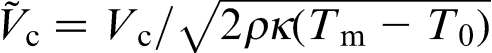
 . According to the normalisation of
 , the relation between t and
 is
is
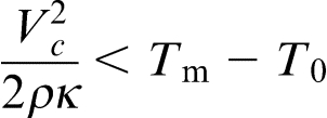
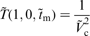
To avoid melting at the contact area, it is important to know the maximum temperature.
 takes the maximum value
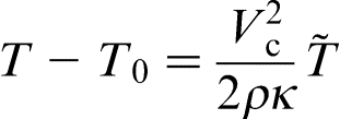
 . The relation between T and
 is
is
 (K), the condition at which the melting temperature is exceeded is
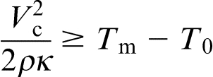
 is defined by equation (30). Since the temperature takes its highest value at the periphery of the contact area,
 satisfies
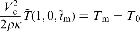
 ; then, equation (35) becomes
 and
and
 have a one to one relation. According to equation (36),
 and
and
 also have a one to one relation; thus,
 and
and
 have a one to one relation. Figure 6 shows
 , where
 satisfies
 from equation (34). It shows that
 monotonically decreases with increasing
 . Therefore, the time to melting is short when
 is large.

Relation between
and

The theoretical time to melting is compared with experimental data.
9
The electric current is passed through a contact area with a diameter of a = 5.0 × 10⁻⁵. The voltage Vc is about 0.19. The literature shows a value of 0.38, but that is for the entire voltage drop for two semi-infinite bodies. The material is gold, so Tm = 1337.33, ρ = 2.3 × 10⁻⁸, κ = 3.2 × 10², and D = 1.3 × 10⁻⁴ at T0 = 300. Thus,
 . From Fig. 6,
 . Thus,
 . The experiment shows that the voltage changes around t = 3.0 × 10⁻⁵. The experimental and theoretical results are of the same order.
Regarding the melting area, when
 , the temperature is higher around the periphery of the contact area. Thus, the melting area is around the periphery of the contact area. The melting range is roughly estimated using Fig. 5a–5c. When
 , the temperature takes almost the same value in the contact area. Thus, the melting area is in the contact area. Regarding the depth range, Fig. 5b shows that the temperature at
 decreases more gradually with respect to
 than at
 . Thus, the melting range is deeper at the centre of the contact area than at the periphery.
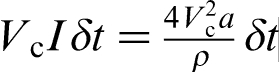
Regarding the total heat generation, which corresponds to the total energy consumption, from equation (14), the heat generation in unit time δQ (J) is
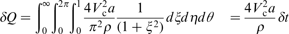
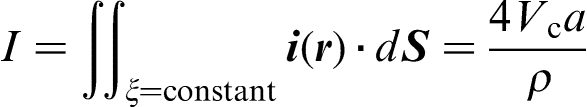
 . From I and Vc, the integration of the heat generated in δt is
 , which corresponds to equation (37).
From equation (37), the total heat generated until melting occurs Q (J) is
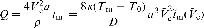
 . Figure 7 shows that
 monotonically decreases with increasing
 . Thus, the total heat generated Q is small when a is small and
 is large. Therefore, we can decrease the energy consumption by choosing a smaller a and larger
 .
.

Relation between Q and
Conclusions
The change in the temperature distribution due to constriction of an electric current through a contact area is analytically and numerically investigated. The potential distribution, current density distribution and heat density distribution are analytically obtained. They are expressed simply by introducing a spheroidal coordinate system.
The current density distribution and heat density distribution have a singular point at the periphery of the contact area. The temperature change rate with respect to time has an infinite value at
 because of the singularity. It is revealed that the temperature has a finite value, whereas the temperature change rate has an infinite value.
The change in the temperature distribution is shown in Fig. 5. The temperature is higher around the periphery of the contact area when
 . Then, the temperature around the centre of the contact area increases and takes almost the same value when
 . From these results, the melting area is concentrated around the periphery of the contact area when
 . The melting range is roughly estimated using Fig. 5a and 5b. This suggests that conventional experimental studies were done under the condition
 , because they reported that the periphery of the contact area melted. When
 , the melting area is on the contact area. The melting range is deeper at the centre of the contact area than at its periphery.
The temperature is in the steady state when
 . The temperature distribution exhibits good agreement with the result of Greenwood and Williamson.
9
When
. The temperature distribution exhibits good agreement with the result of Greenwood and Williamson.
9
When
 , the temperature is almost in the steady state. If the steady state is needed, the condition for the steady state must be satisfied.
The maximum temperature is obtained because there is a steady state condition. Thus, the condition for not exceeding the melting temperature is obtained. The condition for melting is the opposite of the condition for avoiding melting. Under the condition for melting, there is a time to melting
 . The time to melting
 monotonically decreases with increasing
 , as shown in Fig. 6.
The total heat generation Q until the melting point is reached, which corresponds to the total energy consumption, is calculated. The total heat generation Q is proportional to a3 and monotonically decreases with increased
 . Therefore, we can decrease the energy consumption by choosing a smaller a and larger
 .
.