
Abstract
In response to the implementation of a new schedule for iron ore fines in the International Maritime Organization's International Maritime Solid Bulk Cargoes Code, improved measures for the management of moisture have been developed. In particular, prediction of cargo moisture allows management of iron ore fines within the supply chain to facilitate the safe shipping of iron ore fines. An Autoregressive Integrated Moving Average model, augmented to allow for shipment tonnage, has been developed to predict the moisture level from previous shipments of the same product. The model explains about 60% of the moisture variance. It was found that inclusion of other available information, such as ore composition, train/rake assays and recent rainfall at port and mine did not add to the predictive power of the model.
Introduction
In recent years, there have been several maritime incidents where ships carrying iron or nickel ores have foundered, with loss of the ship and in some cases with loss of life.
These recent tragedies, and the potential for further such disasters, have prompted intensive investigations by producers, shippers and regulatory authorities as to the appropriate measures that are needed to prevent future occurrences (Mulrenan, 2012).
In response to these events the International Maritime Organization issued circular DSC.1/Circ.66. It provides an interim framework for iron ore fines while research is completed to guide the formation of regulations for iron ore fines.
Liquefaction
If a granular cargo contains excessive moisture, there is a possibility that it may liquefy in the ship's hold, causing instability that may result in the vessel sinking. The mechanism of liquefaction is complex, but essentially ‘the volume of the spaces between the particles reduces as the cargo is compacted owing to the ship motion, etc.; the reduction in space between cargo particles causes an increase in water pressure in the space; and the increase in water pressure reduces the friction between cargo particles resulting in a reduction in the shear strength of the cargo…Liquefaction does not occur when the cargo consists of very small particles (particle movement is restricted by cohesion and the water pressure in spaces between cargo particles does not increase) nor if the cargo consists of large particles or lumps (water passes through the spaces between the particles and there is no increase in the water pressure)’ (International Maritime Organization, 2012).
Iron ore fines particles are of an intermediate size range where there is a potential for liquefaction if moisture content exceeds a critical level, which is referred to as the transportable moisture limit (TML). Consequently, there is now a clear requirement to be able to verify that the moisture content of an iron ore fines cargo is below the TML.
Iron ore lump shipments have a sufficiently large particle size that liquefaction is not possible.
Moisture management and, in particular, the ability to reliably predict the moisture of a cargo improves the ability of the shipper to comply with the regulatory requirements.
These requirements generate two problems that are exacerbated by high volume supply chains: first, ascertaining the TML appropriate to the cargo being loaded, and second, determining and managing the actual moisture content of the cargo so that it is below the TML when loaded.
Ascertaining the TML
Determining the TML appropriate to the cargo is a complex issue, since it requires understanding of the forces that the cargo is likely to encounter during shipment, and the effect that these stresses are likely to have on the loaded cargo coupled with the material properties. There are three empirical tests that are available in the International Maritime Solid Bulk Cargoes Code to determine TML. Ascertaining the TML is outside the scope of this paper.
Estimating the actual moisture content
The characteristics of high volume iron ore supply chains are such that early decisions for correcting moisture content minimise production losses associated with materials handling and product quality variation. It is therefore necessary either to have sufficiently accurate measurements that can be made in real time or near real-time (therefore the results are available as the ore moves through the port), or to develop a method for forecasting the moisture level of a cargo, informed by recent results, and possibly including other factors such as moisture and rainfall at the mine and/or port.
Microwave measurements, current instrumentation and low frequency microwave moisture analysers have proven unreliable due to calibration issues associated with conveyor bed thickness, particle size distribution and ore mineralogy.
Measurement errors for the major analytes (iron, silica, alumina and phosphorus) are periodically calculated, following the current standard ISO 3085 (2002). Unfortunately, such repeat measurements are not available for moisture content predominantly due to the impacts of porosity and mineralogy on hygroscopic moisture, equilibration and the determination of the true moisture end point. It is estimated that the accuracy of reported moisture assays has a standard relative error of about 0·3% moisture. Since multiple samples are taken for each shipment, their estimates are expected to have greater accuracy.
This paper reports a study examining whether moisture content of each shipment can be accurately forecast from the moisture content of earlier shipments. Potential extensions of the model were examined to find whether the model could be improved by including the assay grade of earlier shipments, and such extraneous information as the rainfall history at the mine and/or the port. The analysis reported has been based upon continuous data for 1852 discrete shipments of an iron ore fines product across the period November 2006 until August 2012.
Forecasting moisture content
A smoothed plot of the moisture level for shipments over the study period shows that there are quite long term trends in the data (Fig. 1), indicating that individual shipments may be able to be forecast from previous values. The general upward trend may be explained by more ore coming from below the water table, and by changes of ore stratigraphy.
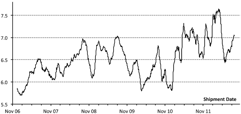
Shipment moisture, 30 ships moving average
Shipment moisture from the previous 1852 shipments had a mean of 6·57 and a standard deviation of 0·561.
Forecast delay
The average interval between shipments was 1·15 days. Information from the previous shipment may not yet be available when the next ship is loaded, so delays of 1, 2 or 3 shipments will be considered (corresponding to average delays of 1·15, 2·3 or 3·45 days).
Naïve forecast
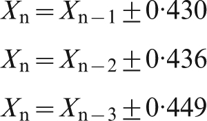
Given the sustained trends in the data, the simplest form of forecast is a naïve model. For this model, the moisture of each shipment is forecast as equal to that of the previous shipment for which moisture data is available. Information delays of 1, 2 or 3 shipments gave
Simple regression
A simple linear regression, allowing an intercept as well as the coefficient, improves the fit. Information delays of 1, 2 or 3 shipments gave
Autocorrelations
The autocorrelation of a time series is the correlation of the values with previous lagged values. For zero lag the autocorrelation is therefore 1·0. The behaviour of the autocorrelation function (ACF) as the lag increases can provide information as to a suitable forecasting model.
The partial autocorrelation function (PACF) at a given lag is the autocorrelation after correction for information carried by the lesser lags. For example, with a first order Markov process each value is probabilistically determined only by the previous value. If we have an 80% chance of buying the same toothpaste as last time, the ACF for lags {1, 2, 3,…} would be {0·8. 0·64, 0·512,…}, but the PACF would be {0·8, 0·0, 0·0,…} because the second and subsequent lagged values carry no information beyond that provided by the first lagged value. The kth PACF is equivalent to the coefficient bk in the regression equation

The ACF and PACF are more fully explained in, for example, Diebold (2008).
ACF and PACF for shipment moisture
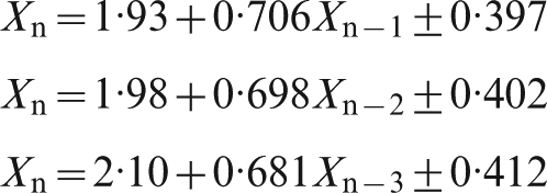
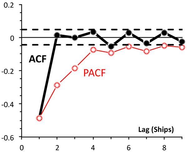
The ACF and PACF for the shipment moisture values are shown in Fig. 2. The parallel broken lines show the 95% confidence limits series (±two standard deviations) if the autocorrelation of a series of random numbers were calculated. Observed correlations therefore have to lie outside the parallel broken lines to be meaningful.
ACF and PACF for shipment moisture
We see that the PACF is significantly different from zero for lags 1 through 4, but then becomes insignificant. The ACF dies away slowly because each value's influence passes through its successors, only slowly dying away.
Because the PACF has died away to the random confidence limit by lag 5, we can say that there is no evidence that the fifth and subsequent lagged values provide significant information that is not already provided by the first four lagged values.
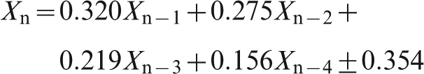
This finding suggests a regression model based on the first four lagged values. For information delays of 1, 2 or 3 shipments, we find
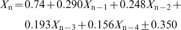
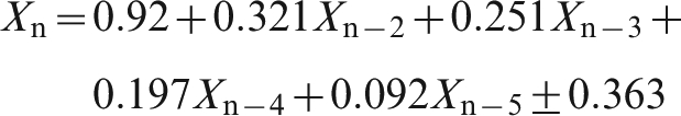
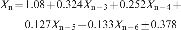
These regressions all have standard errors that show an improvement on the standard error for the simple regressions. As to be expected, a greater information delay again somewhat increases the standard error of the forecast.
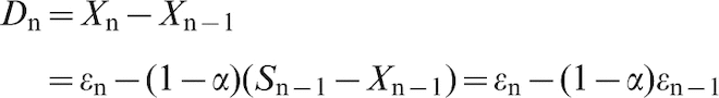
First differences
We define the first difference Dn = Xn–Xn–1; and the ACF and PACF for the first differences are shown (Fig. 3).
ACF and PACF for first differences
In this case, the ACF becomes insignificant after the first lag; but the PACF remains significant for the first four lags. This is an example of the not uncommon situation in a regression model where a variable on its own has little predictive power, but becomes predictive once another variable has entered the model.
We can construct regression model based on the first three lagged values. For information delays of 1 shipment, we find
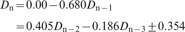
Replacing Dn–k with (Xn–Xn–k–1) gives
Interestingly, equation (8) is identical to the result obtained if equation (4) is run again, forcing the intercept to zero (increasing the standard error from 0·350 to 0·354).
Autoregressive integrated moving average (ARIMA) models
The models so far examined (plus many others published under a variety of names) are examples of a generalised set of ARIMA models first categorised by Box and Jenkins (1970). These models combine autoregressive (AR), moving average (MA) and integrative (I) elements.
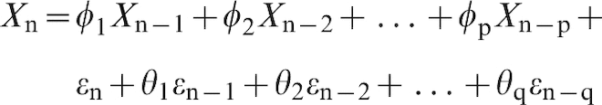
An MA(q) moving average process of order q is

The moving average is thus the weighted average of a series of random shocks ϵn.
An AR(p) autoregressive process of order p is

The autoregressive process is therefore a regression model, with the independent variables being the previous values of the process.
Combining the two provides an autoregressive moving average ARMA(p, q) process
A first order integrated ARIMA(p, 1, q) process is an ARMA(p, q) applied to the first differences Dn instead of the values Xn
If the differencing is done d times, then we have an ARIMA(p, d, q) process. For the models developed so far in this paper, equations (1) to (6) gave examples of ARIMA(p, 0, 0). Equation (7) was an ARIMA(3, 1, 0) process, which could be reformulated in equation (8) as an ARIMA(4, 0, 0).
Error terms
In this paper, error terms are expressed as ϵn if they refer to theoretical populations, and as en if they refer to sample observations.
Exponential smoothing models
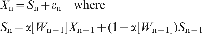
Exponential smoothing models are used for both forecasting and control. They have proven useful for both purposes in maintaining iron ore quality (Everett, 2007; Everett and Howard, 2011). For an exponential smoothed process

Equation (13) can be rewritten as
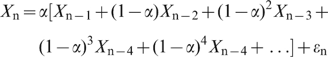
Therefore exponential smoothing is expressible an ARIMA(∞, 0, 0) process. However, equation (13) can also be written as

This is a finite ARIMA(0, 1, 1) process. Being a more parsimonious formulation than ARIMA(∞, 0, 0), it is preferable to identify exponential smoothing as being an ARIMA(0, 1, 1) process.
One advantage of an exponential smoothing is that the history does not need to be remembered: only the current observation Xn and the current smoothed value Sn are required.
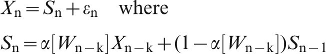
Allowing for information delay
If assay information is delayed by k shipments (so when ship n is being loaded we have moisture assays for ship n–k) then the exponential smoothing becomes

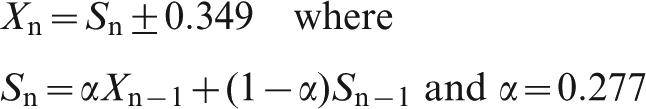
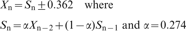
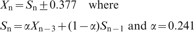
Exponential smoothing to forecast the moisture data
Applying the exponential smoothing model to the moisture data, we adjust the parameter alpha so as to minimise Σen2. For information delays of 1, 2 or 3 shipments, we find
Summary for basic ARIMA models
The analyses discussed above have used a range of ARIMA models, and are summarised (Table 1).
ARIMA model results
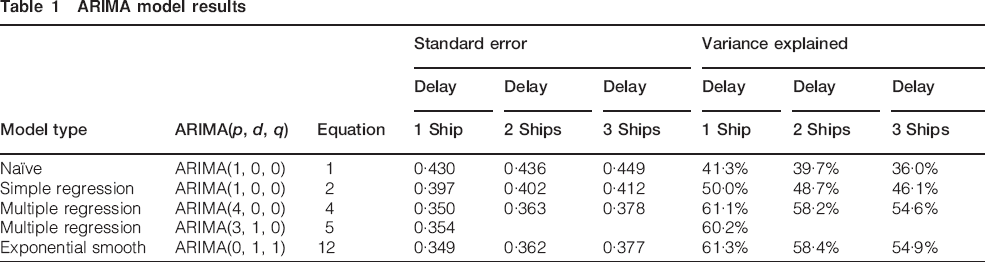
The exponential smoothing model gives the smallest standard error. It is also the simplest to apply.
In all of the above models, we have ignored the effect of varying shipment tonnage. The effects are two-fold. One effect of varying tonnage is that we would expect smaller errors for larger tonnage shipments. This can be corrected for in any of the models by using weighted least squares rather than ordinary least squares as the objective function to be minimised. A second more subtle effect is that when forecasting a shipment, shipments of larger tonnage should have more influence. Modification to allow for this second effect is difficult for a regression model but, as we shall see, can be readily incorporated into the exponential smoothing model.
Exponential smoothing including shipment tonnage
Smoothing factor increases with tonnage
For most textbook examples of time series analyses, it is assumed that successive observations are of equal importance. For iron ore shipments (parcels of ore of varying tonnage) this assumption is clearly inappropriate, since any of the ARIMA models considered would lead to a different forecast value if the previous two shipments were consolidated into a single shipment.
To overcome this problem with an exponential smoothing model, it is necessary to make the smoothing factor α be a function of the shipment tonnage (Everett, 2007). For consistency, if the nth shipment has tonnage Wn, and α1 is the smoothing factor that would be applied to unit tonnage, then

Equation (13) becomes
Error variance decreases with tonnage
The unit smoothing factor α1 needs to be selected so as to minimise the error variance. For an ordinary least squares solution, this is done by minimising Σen2.
The error variance is expected to be less for larger tonnages, and it is not unreasonable to assume that the error variance is inversely proportional to the shipment tonnage.
We shall therefore use a weighted least squares approach, by minimising ΣWnβen2, with the condition that Wnβen2 is independent of Wn.
Allowing for information delay
If assay information is delayed by k shipments (so when ship n is being loaded we have moisture assays up to ship n–k) then the exponential smoothing becomes
Exponential smoothing to forecast the moisture data
The exponential smoothing model was applied to the moisture data, for information delays of 1, 2 and 3 shipments respectively. For each analysis, α1 was adjusted to minimise ΣWnβen2, with the exponent β being constrained so that the correlation between Wnβen2 and Wn is zero.
Results
The optimum parameters for information delays of 1, 2, or 3 shipments are reported (Table 1). The average delay between shipments was 1·15 days, so 1, 2, or 3 shipment intervals correspond to an average of 1·15, 2·30 and 3·45 days respectively. The α1 and β parameters are chosen so as to minimise ΣWnβen2. The optimum alpha value corresponds to smoothing over about 300 kt ( = 1/0·0033).
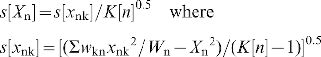
The value of Wβϵ [W]2 is estimated as ΣWnβen2/N, where N is the total number of shipments. The overall standard error is reported (Table 2). Applying the parameters, the standard error of the forecast for a shipment of tonnage W kt can be estimated as

Exponential smoothing parameters
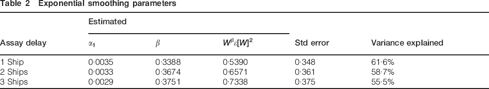
The estimated ϵ[W] as a function of W for information delays of 1, 2, or 3 shipments, where the average shipment interval is about 1·15 days is shown (Fig. 4). Increasing the information delay does increase the standard error of the forecast, but not by very much. The standard error decreases with shipment tonnage as shown.
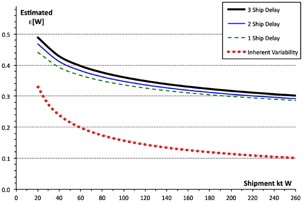
Standard error of forecasts, for information delays of 1, 2 or 3 ships
Inherent variability
The dotted line in the lower part of Fig. 4 shows the variability inherent in the shipments. The moisture of each shipment Xn was calculated from a number K[n] of samples, of weight wkn and moisture xkn
The number of samples, K[n], per shipment ranged from 2 to 18. The samples within each shipment varied, indicating either measurement error or variability within the shipment (or probably both). Consequently, there is an inherent variability to each shipment's moisture with a standard deviation equal to the standard deviation of the shipment mean, derived from the within-shipment standard deviation. No forecasting system would be able to do better than this inherent variability, so plotted as a dotted line (Fig. 4), the inherent variability provides a baseline to the forecast.
For each shipment, the standard deviation of the shipment mean was calculated as
The inherent variability is expected to decrease as the shipment tonnage increases. The standard deviation of the shipment mean s[Xn] was therefore fitted to a function of the form pWnq. The coefficients p and q were selected so as to minimise the summed squared residuals, weighted for each shipment by the degrees of freedom (K[n]–1).
The best fit gave coefficients p = 1·3134, q = −0·4618. Therefore, the inherent variability (Fig. 4) is the function 1·3134W−0·4618. It is of interest that, if the sample moistures within a shipment had no autocorrelation, we would expect q to be −0·5. Positive autocorrelation between them would diminish the magnitude of q, so the result that q = −0·4618 is credible.
Measurement error
The international standard ISO 3085 (2002) prescribes precision testing for the chemical components of iron ore, but not for moisture. Consequently, we have no information as to the measurement error applicable to a moisture assay, although the standard error for a sample is assumed to be about 0·3.
From equation (26), the appropriately weighted mean of s[xnk] is 0·478, and this can be taken as the upper bound for measurement error. The error for a shipment, comprising multiple samples would be less than this, to the extent that sample assay errors are independent.
The measurement error should decrease with increasing shipment tonnage, since it usually involves more samples. It should be realised that the measurement error provides a lower bound to the apparent forecasting error: even a perfect forecasting procedure would report apparent errors equal to the measurement error.
The inherent variability (Fig. 4) is an upper bound to the measurement error for shipments.
Error analysis
Before deciding to use the modified exponential smoothing model to forecast shipment moisture values, we need to investigate whether the distribution of errors is well behaved. This includes checking whether the error distribution has changed over the period of the study, and whether it is skew or long-tailed, or approximates a normal distribution.
For each of the three models (information delay of 1, 2, or 3 shipments), standardised z-scores were calculated for each shipment (zn = en/ϵ[Wn]).
Changes in error variance across time
The standardised error variance (zn2) was exponentially smoothed across the entire data set. The variability of zn2 about the trend was minimised with an exponential smoothing factor of 0·0001/kt, equivalent to smoothing over 10 million tonnes, or about 100 shipments. The smoothed value of the standardised error variance was converted to the forecast standard error for 100 kt shipments, according to
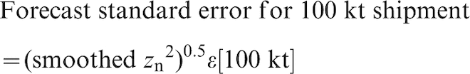
Changes in standard error across time, for 100 kt shipments
Distribution of the forecast errors
The cumulative probability of the z-scores after adjustment was calculated as

The cumulative probability distribution of the z-scores after adjustment is shown for information delays of 1, 2 or 3 shipments, and also for the standardised normal distribution (Fig. 6). Errors around the forecast (adjusted for variation across time and shipment tonnage) are very close to being normally distributed.

Probability distribution of forecast errors, after adjustment for time and tonnage
Application of the model
The model as described can be applied to forecasting the moisture content of a product, with the standard error of the forecast being exponentially updated as time proceeds. When the model is applied to another ore product, appropriate α and β parameters need to be established, following the methodology described.
The error distribution very closely approximates a normal distribution (Fig. 6). Therefore, as a one-tail test, the upper 95% confidence limit for moisture level Xn is the forecast value Sn plus 1·645 times the standard error. The upper 99% confidence limit is the forecast value plus 2·326 times the standard error. The standard error is a function of shipment tonnage (Fig. 4).
The upper 95% and the 99% confidence limits of the forecast values for each shipment is shown, assuming a three-shipment delay before assays are available (corresponding to about four and a half days; Fig. 7).
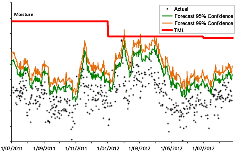
Actual, 95 and 99% Forecast Confidence Limits, and the TML
The confidence limits for each shipment include allowances for the dependency of forecasting errors on shipment tonnage (Fig. 4) and on the variation across time (Fig. 5).
For comparison, the actual moisture values and the TML are also plotted (Fig. 7). The only occasion when the actual moisture content approached the TML was in late January 2012. On this occasion, the forecast confidence limits would have provided clear warning.
The model can clearly be seen to provide a conservative approach to predicting the moisture value of subsequent shipments. The 95% confidence level of the model performs well by overestimating and therefore reducing the risk.
The powerful predictive capability of this model is being integrated into the moisture management process at BHP Billiton's Port Operations at Port Hedland for all iron ore fines products.
Other possible predictors
We examined the potential for further augmenting the forecasting model, to include other predictors of moisture. This was achieved by correlating the residuals of the current model with each of the candidate variables. The candidate variables included recent rainfall at the mine, recent rainfall at the port, and assay grades (for analytes other than moisture) for recent shipments. None of the candidates tested gave significant correlations with the residuals of the model. We therefore concluded that these candidate variables could not be used to improve the model.
Conclusions
This paper has discussed a range of ARIMA models for forecasting moisture content for iron ore shipments. An exponential smoothing model, ARIMA(0, 1, 1) has been found to be the most accurate and simplest to implement of the models considered. The model has been augmented to allow for the effect of varying shipment tonnage on the influence of recent shipments, and allow for the effect of varying shipment tonnage on the error variance.
The appropriate influence of varying shipment tonnage has been shown to require a smoothing factor of about 1/300 kt, which means the influence of preceding shipments has a half-life of about 300 kt, or about three cargoes on average.
The error variance has been shown to decrease with increasing tonnage W according to a ratio W−β , where β is in the range 0·33 to 0·38. This value for β makes sense, because if the sampling variation (real plus error) within each shipment were independent, then β would be one, whereas if the sampling variation within each shipment was fully dependent β would be zero.
The forecast error increases only slightly as the information delay between assays being taken and results being available increases from 1 to 3 shipments. These shipment delays correspond to an average of 1·15, 2·3 or 3·45 days.
The forecast error variance depends not only on shipment tonnage, but also to vary across time. This variation with time has been identified, and the methodology provides for its continual update.
After adjustment for time and for shipment tonnage, the forecast errors are found to be very close to a normal distribution. Accordingly, if the moisture forecast is at least 1·645 standard errors below the TML, then we can be 95% confident that the TML will not be exceeded. For 99% confidence, the moisture forecast needs to be at least 2·326 standard errors below the TML.
In the absence of methods for measuring and reporting moisture in real time (or near real time) the methodology described appears to provide sufficiently accurate predictions of moisture and has been adopted as the basis for a prediction tool for routine use in planning the dispatch of BHP Billiton's iron ore shipments from Port Hedland.
Further study, not covered in this paper, is needed to refine the estimation of the TML for the relevant ore. It would also be desirable to establish the measurement error when the moisture content of an iron ore sample is assayed. It may appear surprising that no routine assessment of precision is carried out for moisture. However, the impacts of porosity and mineralogy on hygroscopic moisture, equilibration and the determination of the true end point contribute to the issue.
The model clearly demonstrates capacity to predict moistures of cargoes and it is being integrated to the moisture management processes at port operations.
Footnotes
Acknowledgements
The authors wish to thank BHP Billiton Iron Ore Ltd and the Australasian Institute of Mining and Metallurgy for permission to publish this manuscript, which was originally presented at the AusIMM Iron Ore Conference in Perth in August 2013.