
Abstract
Brockman 4 is a large iron ore deposit hosted by the Brockman Iron Formation in the Pilbara region and is mined by Rio Tinto Iron Ore. Drilling is mainly by the reverse circulation method and samples are taken at 2 m intervals using a rotary cone splitter or historically by riffle splitter. Samples are geologically logged, assayed by X-ray fluorescence for iron, silica, alumina, phosphorus, manganese, sulphur, titanium oxide, calcium oxide, magnesium oxide, and 19 other trace elements; and measured for loss on ignition by thermogravimetric analysis. Mineralisation is estimated by ordinary kriging with unfolding and waste by inverse distance interpolation. The model is validated, reconciled with historic production, classified according to the 2012 Edition of the JORC code and stored in a SQL Server database.
Keywords
Introduction
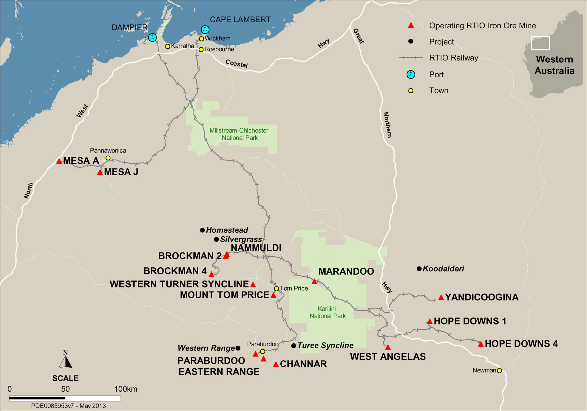
Rio Tinto Iron Ore (RTIO) operates 15 open cut mines in the Pilbara region of Western Australia with a current annual capacity of 237 million tonnes and there are plans to increase capacity to 330 million tonnes by 2015. The Pilbara operations make up an integrated system of fifteen iron ore mines, three shipping terminals and a heavy freight rail network (Rio Tinto, 2013a). Rio Tinto fully owns Hamersley Iron's eight mines (Brockman 2, Brockman 4, Marandoo, Nammuldi, Paraburdoo, Tom Price, Western Turner Syncline and Yandicoogina) and operates seven joint ventures mines: at Hope Downs 1 mine (Rio Tinto 50%), Hope Downs 4 mine (Rio Tinto 50%), Channar mine (60%), Eastern Range (54%), and in the three mines of Robe River Iron Associates which are Mesa J, Mesa A-Warramboo and West Angelas (53%). A centralised control room in an Operations Centre is located near Perth Domestic Airport (Walsh, 2010). The Operations Centre allows management of mines, port and rail assets from a single location 1500 km from the mines and is an important part of the Mine of the Future program (Rio Tinto, 2013b). The Mine of the Future program develops improvements to the mining process with increased automation and use of remote operations. The program helps increase efficiency, lower production costs, improve health, safety and environmental performance, and offers better working conditions.
The Resource Evaluation Division in RTIO undertakes drilling programs which cover existing operations, operating mine lease exploration, new mine developments, development studies, tenure security and new tenement development. It includes hydrogeological, geotechnical and geometallurgical drilling and analysis. Over the last four years, the total number of metres drilled has more than doubled to support the increased rate of mining: from 306 km in 2009 to 615 km in 2012. The total metres drilled in 2012 are 16 times greater than in 2000 when 38 km were drilled. The orebody knowledge gained from drilling allows the creation of new geological models or the update of existing models using the new data.
The geological block models created or updated by the Resource Evaluation Division are estimated using ordinary kriging by the Resource Geology Estimation Department within RTIO. The number of resource models continues to increase in line with the increase in drilling metres.
Total Mineral Resources for RTIO, as at 31 December 2011, are estimated to be 18 441 Mt at 59·9% Fe in addition to the Ore Reserves of 2876 Mt at 61·3% Fe (Rio Tinto, 2013c). The Resources and Reserves comprise Bedded Marra Mamba Formation and Brockman Iron Formation deposits, Tertiary detrital deposits and channel iron deposits.
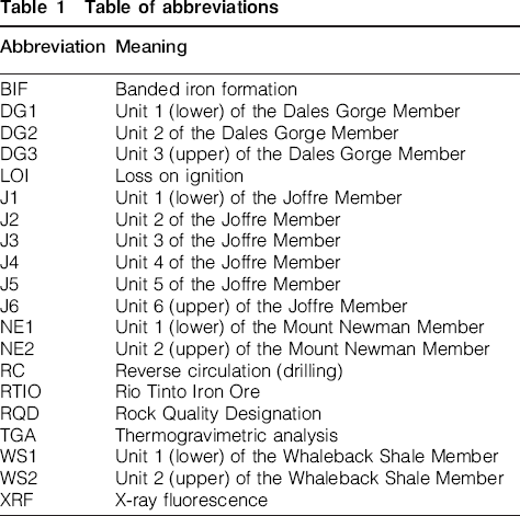
This paper presents the methodologies used in estimating the Brockman 4 (BS4) deposit, which is found approximately 55 km west of the town of Tom Price (Fig. 1). This is a typical example of the resource estimates performed by the Resource Estimation Department and demonstrates the methods utilised. Table 1 lists abbreviations used in this paper.
Location of the BS4 deposit
Table of abbreviations
Geological constraints of the resource model
Trendall and Blockley (1970) provide documentation of the stratigraphy and are summarised below. The BS4 deposit is within the Mount Bruce Supergroup which is made up of three groups: Fortescue, Hamersley, and Wyloo (oldest to youngest). The Hamersley Group is around 2400 m thick, consists of abundant banded iron formation (BIF) with interstratified acid lavas dated at 2000 Ma years old, and hosts the bedded iron ore deposits in the Pilbara region. The Hamersley Group is made up of the following formations (oldest to youngest with thickness): Marra Mamba Iron Formation (180 m), Wittenoom Dolomite (150 m), Mount Sylvia Formation (30 m), Mount McRae Shale (90 m), Brockman Iron Formation (600 m), Weeli Wolli Formation (300 m), Woongarra Volcanics (730 m) and Boolgeeda Iron Formation (200 m). The BS4 deposit is hosted by the Brockman Iron Formation, which is made up of four members (with thicknesses): Dales Gorge Member (150 m), Whaleback Shale Member (60 m), Joffre Member (360 m), and Yandicoogina Shale Member (60 m). Enrichment of the host member BIF units is thought to have occurred through the supergene process as described by Morris (1985).
The Dales Gorge Member and Joffre Member consist of alternating macrobands of banded iron formation and shale. They are informally divided by RTIO using positions of shale bands into units known as strands. The Dales Gorge Member is stranded into three sub-units (lower to upper): DG1, DG2, and DG3. Similarly, the Joffre Member is divided into (lower to upper) J1, J2, J3, J4, J5 and J6. The units J1, J3 and J5 are more dominated by shale, whereas J2, J4 and J6 are more dominated by banded iron formation. The most iron enriched part of the Marra Mamba Iron Formation is the Mount Newman Member and this member is divided into the NE1 and NE2 units. NE2 may be further divided into N2U and N2L. These strands form the fundamental domains for Mineral Resource estimation. Each strand is further divided into mineralised non-hydrated, mineralised hydrated and non-mineralised domains.
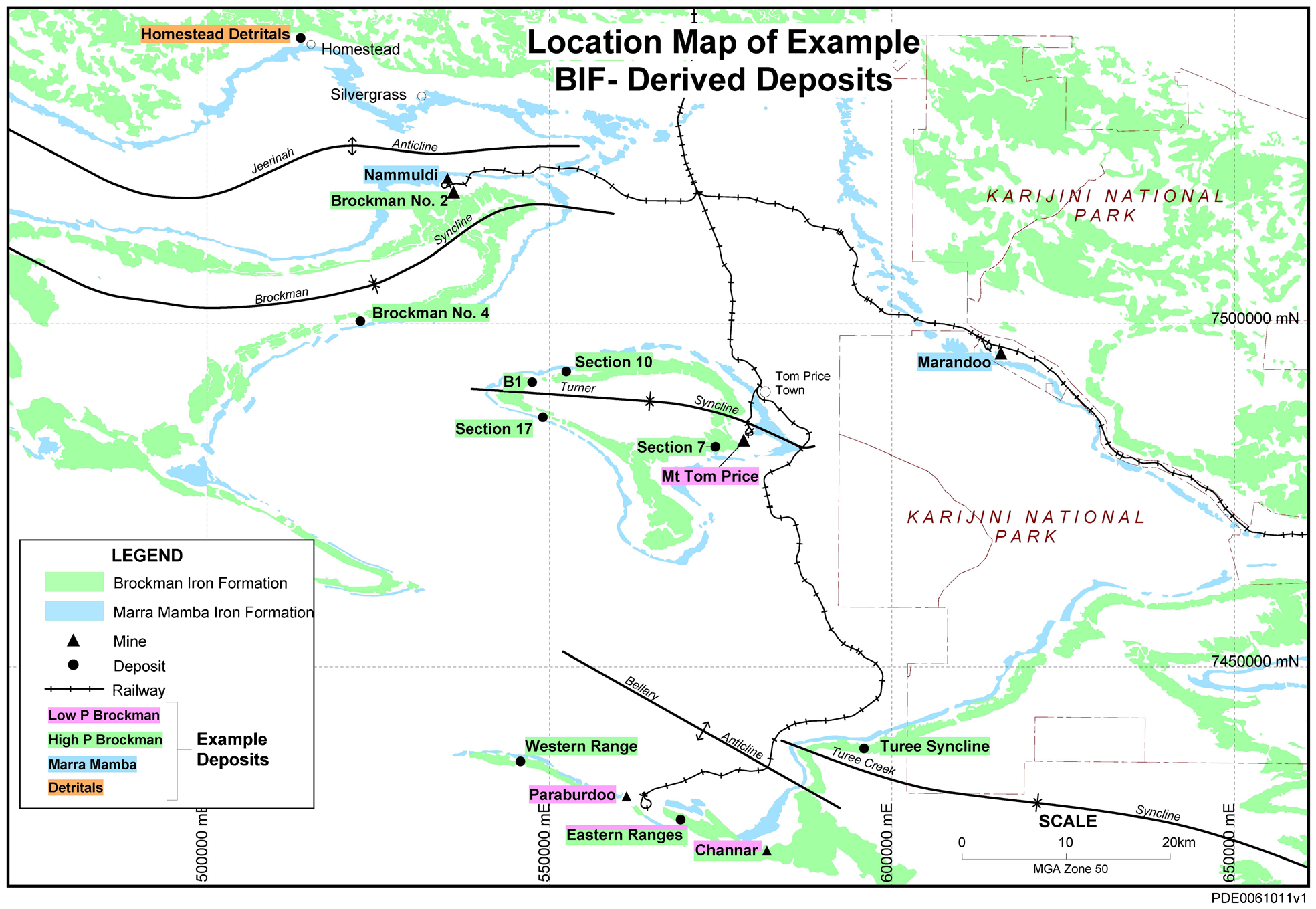
The BS4 deposit is located on the southern limb of the large scale Brockman Syncline (Fig. 2). BS4 mineralisation is dominated by martite-goethite and is of the high phosphorus ore type. Mineralisation is hosted by the Dales Gorge, Whaleback Shale and the Joffre Members of the Brockman Iron Formation over a strike length of approximately 14 km with mineralised thicknesses of up to 240 m. The deposit is divided into three main lenses: West, Central and East. The stratigraphy in the deposit dips north at around 40 degrees. A typical geological cross-section is shown in Fig. 3. Mineralisation is hydrated from surface to a depth of 10 to 30 m. Mineralisation is generally flat lying but can follow the Whaleback Shale contact down dip in a steeper orientation to considerable depths. Though most mineralisation is bedded, there are small deposits of secondary surficial detrital mineralisation present above the bedded mineralisation. There are numerous steep, northwest striking, normal faults at BS4. Bedding is openly folded and is also sharply kinked near the faulting. Dolerite dykes are common, strike northwest and often intrude faults.
RTIO BIF derived deposits in the Pilbara region of Western Australia
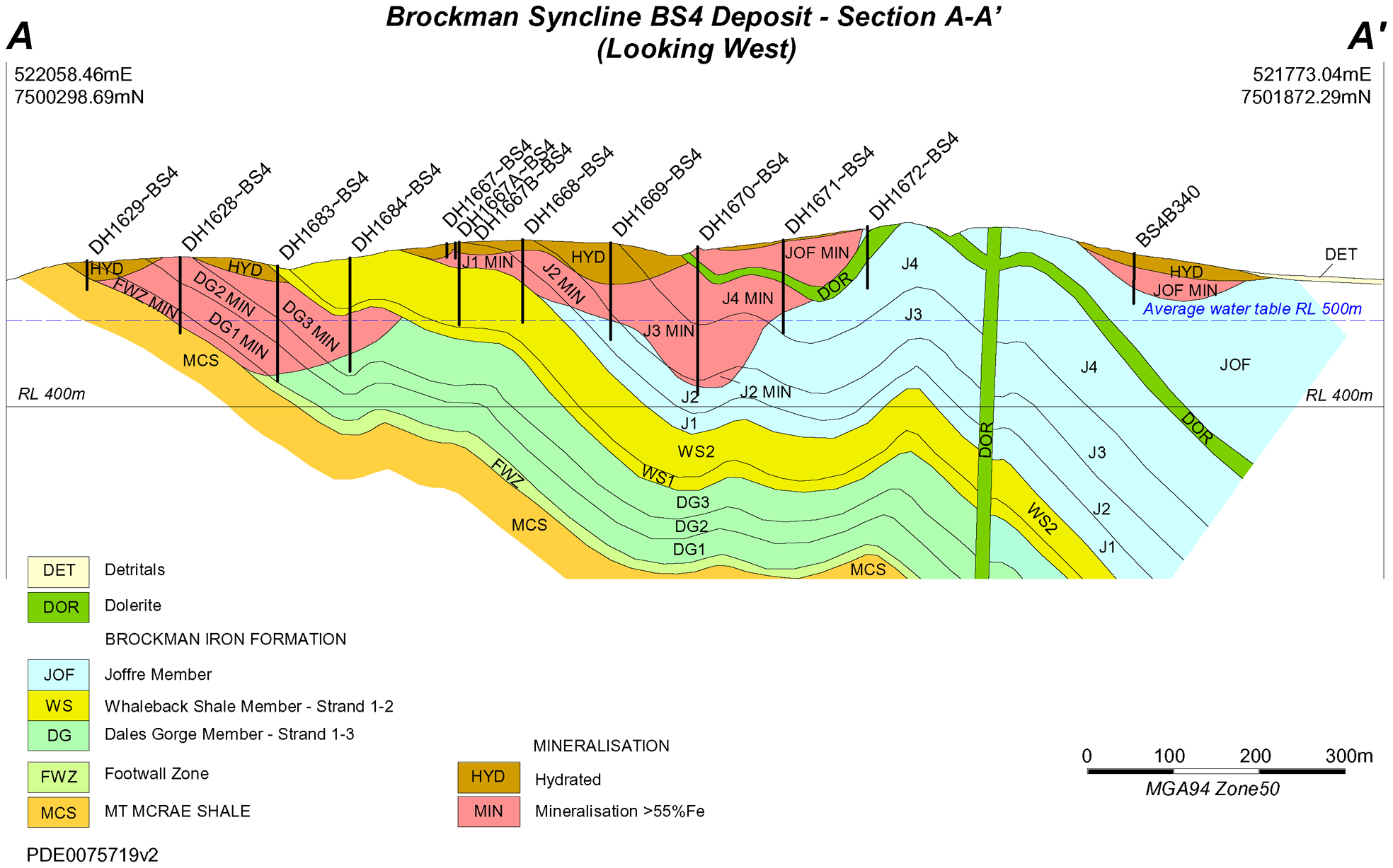
Cross-section of BS4 deposit geology
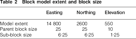
A geological interpretation is carried out based on information obtained by drilling and supported by other field data such as surface mapping. At the scale of the drill hole, the geological strands are interpreted based on natural gamma traces. Shale bands have elevated natural gamma readings and these peaks in the natural gamma traces are used to correlate shale bands across the deposit and determine where they lie in the stratigraphic sequence. Geological wireframes corresponding to the base of the strands are created from drill hole contact points and are used to build the geological block model. Mineralised intervals in the drill holes are identified based on assays and logging data, and these are domained into different geozone codes. The geozone field is a numeric field that is based on geological unit and whether the interval is non-hydrated mineralisation, hydrated mineralisation or un-mineralised. Geozone values are stored in the main acQuire drill hole database rather than being coded from wire frames. The geozone field is used to ensure that all the samples that spatially intersect a modelling domain are grouped together and used in the grade estimation of that domain. A wireframe is also created to represent the boundary between mineralised material and waste at a cut-off grade of around 50% iron. The cut-off grade for iron is more flexible in the hydrated zone than in the non-hydrated areas due to the greater internal variability in the hydrated zone. Small intervals of waste of less than 6 m length down hole may be included within the mineralised domain to improve continuity. Geological surfaces representing stratigraphy and faults (where present) are used to flag a geological block model built using Vulcan software. Models of BS4 are built at a primary block size of 25 m along strike, 25 m across strike and 5 m vertically, with sub-celling to a quarter of the parent block size. Sub-celling is used as it allows more accurate volume calculations. Table 2 shows the model extent, parent block size and sub-block size.
Block model extent and block size
Drilling
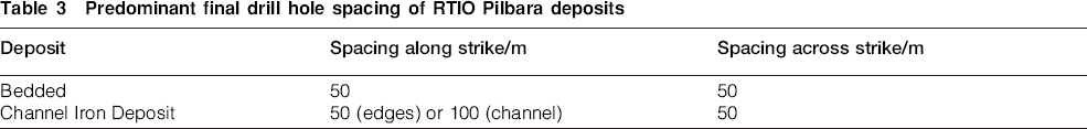
Drilling is at a spacing of 50 m by 50 m in the Western Lens, Central Lens and on the western side of the Eastern Lens; and at 50 m by 100 m on the eastern side of the Eastern Lens. The spacing of 50 m along strike by 50 m across strike is one of the common final drill hole spacings for RTIO Pilbara deposits (Table 3). Drilling data for the BS4 model consist of 3673 reverse circulation (RC) drill holes, 213 open hole percussion drill holes and 5 HQ size diamond drill holes. Drilling has taken place from 1963 to the present.
Predominant final drill hole spacing of RTIO Pilbara deposits
Sampling
RC holes are currently sampled using rotary cone splitters though in the past riffle splitters were also used in dry intervals. Recoveries of RC samples are qualitatively estimated from the size of reject piles and sample weights. Diamond drilling uses water and polymer mud to maximise recovery of cores. Diamond core recovery data is recorded and there is good recovery, greater than 98%, for all holes. Any intervals of core loss or cavities greater than 5 cm are recorded and marked by the driller. Run lengths vary depending on material with short runs employed to maximise recovery of soft or friable material including shales.
RC holes and early percussion holes are geologically logged with peer review and validation during the drilling programs. Material is sampled and assayed for each 2 m interval. Currently each 2 m RC interval is geologically logged and entered into an offline acQuire database package on field Toughbook laptops, with later upload to the main acQuire database. Before 2006, logging was recorded on paper logs. Standard colour, texture, hardness, shape, chip percentage descriptors and a comments field are used for logging. Iron ore material types are logged with percentages usually recorded in increments of 5% and rarely at 1% increments for trace constituents. Material types are differentiated by mineralogy and texture. Logging is validated against the assays using an in-house validation tool. Magnetic susceptibility readings are taken using a Kappameter for each interval. Diamond core is geologically logged on 2 m intervals. Core loss and core recovery, RQD, fracture count and hardness are recorded along with standard descriptors as used with RC logging. Both the RC and diamond core are logged in accordance with the RTIO material type classification scheme.
Assaying
Samples are dispatched to the Ultratrace laboratory in Perth, and are sent in batches of 200 to 300 samples. The samples are oven dried, crushed and then pulverised to a uniform size range. The pulverised fraction is then further split. The flux is a mix in a ratio of 12∶22 of Lithium Tetraborate (35·3%)/Lithium Metaborate (64·7%) and weighs 7 g. Flux is mixed with 0·66 g of pulp sample in a platinum crucible, and undergoes robotic fusion at 1050°C with the melted material poured into a mould to make the glass bead for XRF analysis. XRF was used to analyse aluminium oxide, arsenic, barium, calcium oxide, chlorine, cobalt, chromium, copper, iron, lead, magnesium oxide, manganese, nickel, phosphorus, potassium oxide, silicon oxide, sodium, strontium, sulphur, tin, titanium oxide, vanadium, zinc, and zirconium. LOI determination is by thermogravimetric analysis (TGA) using a multi-furnace robotic cell on a separate split of the pulverised fraction. The assaying work flow at ultratrace for RTIO XRF samples is summarised below:
dry for minimum of 24 h
weigh
crush in a Boyd Crusher to 90% passing −3 mm
pulverise in an LM5 to 95% passing 150 μm
sample fusion and TGA weighing
weigh sample into RTGA crucible
weigh flux and sample into crucible
robotic fusion
XRF analysis
XRF QA/QC.
Density
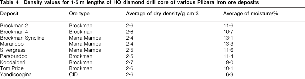
Continuous down hole geophysical logging is used for RC and diamond drilling to record gamma–gamma density and hole width from calliper readings. Wet and dry diamond core density is also obtained using a volumetric approach where the weight of core is divided by its volume. Table 4 shows the average values for dry density and moisture of 1·5 m diamond drill hole composites for a number of Pilbara deposits. Much more data is collected from continuous gamma–gamma density measurements than for core samples from diamond drilling. The average density values, split by domain and into above or below water table, are compared for the gamma–gamma density data and the diamond core data. This allows a correction factor to be determined to adjust the gamma–gamma density to dry bulk density. This correction is required as the gamma–gamma density measures wet density, whereas resource models require dry bulk density. Scatter plots are made of RC gamma density versus dry core density and a linear regression trend line is fitted to the data to allow conversion of gamma density to the dry core density equivalent.
Density values for 1·5 m lengths of HQ diamond drill core of various Pilbara iron ore deposits
Compositing
Most samples are 2 m in length though there are some diamond drill hole samples with variable lengths. Compositing is done to 2 m lengths down the hole without splitting by geological boundaries. Average grades of samples versus 2 m composites were compared for each geozone and there are small differences of up to 0·01 relative per cent in some elements for mineralised J5, J4, WS1 and DG1 domains. Each geological unit is divided into mineralised non-hydrated, mineralised hydrated and non-mineralised domains for statistics, variography and estimation.
Contact analysis
Contact analysis is used to examine the change of chemical grades across geology and hydration boundaries. The average grades of composites at various distances either side of geological contacts are charted to show if there is a gradational or step change in grade across the contacts. Contacts between geological units are defined by highly continuous and distinctive shale bands which are clearly seen in geophysical logging of natural gamma radiation. There are also sharp chemical boundaries and step changes in grades between aluminous shale bands and more siliceous banded iron formation. The boundary between hydrated and non-hydrated mineralised domains is moderately well defined by logging of material types and chemistry. Hydrated domains have higher silica and alumina, and less distinctive down hole geophysical logs of natural gamma than the adjacent non-hydrated domains. The boundary at the base of the hydrated is fairly well sharp and the hydrated material has lower iron and higher silica (Fig. 4). Contact analysis shows a relatively well defined chemical boundary ore and waste within the Dales Gorge, Joffre and Whaleback Shale Members.
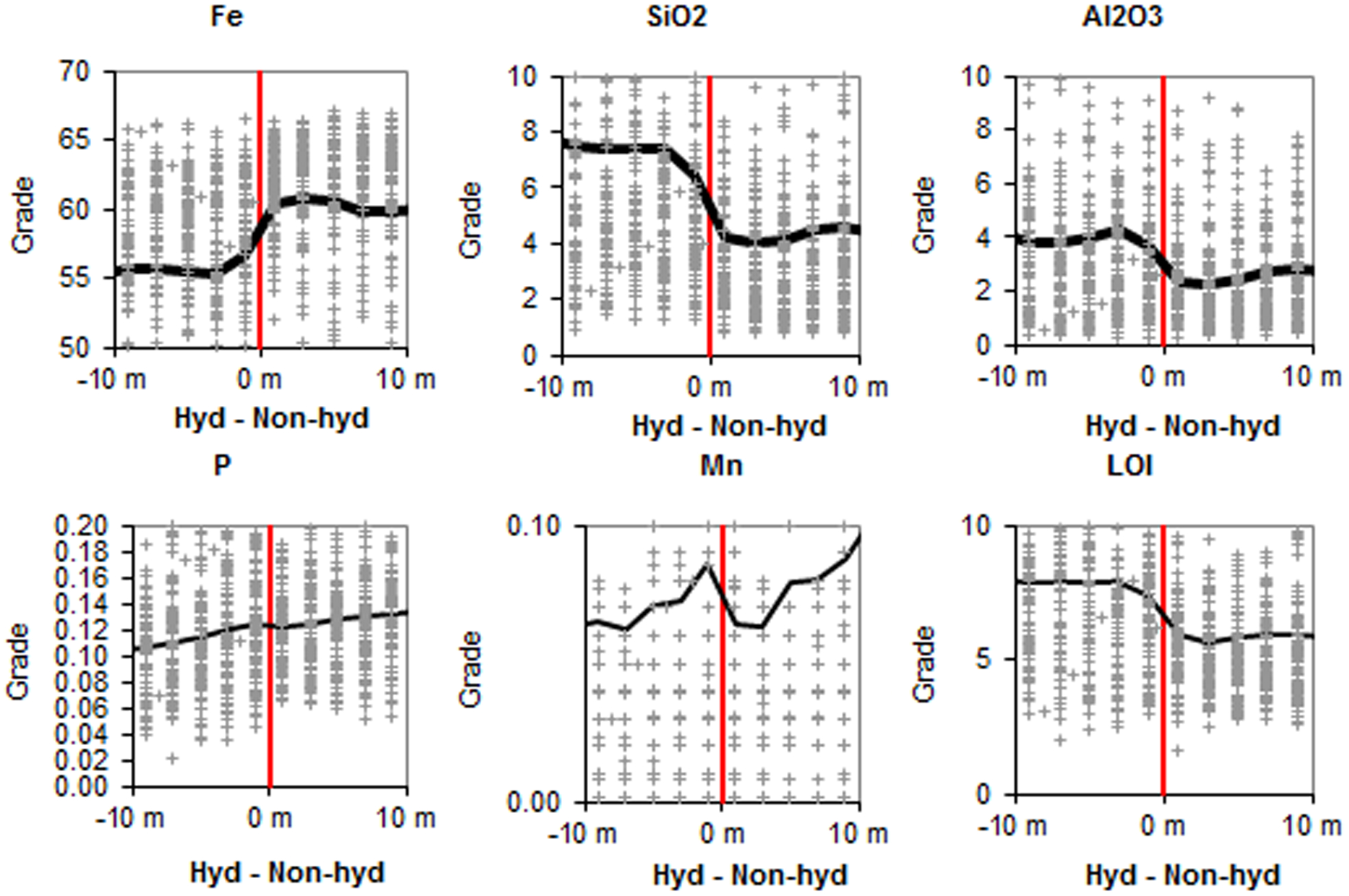
Contact analysis chart for the contact between hydrated mineralisation to non-hydrated mineralisation, with the grades of individual samples (crosses) and average grades of samples (black lines) from 10 m before to 10 m after the contact (red lines)
Contact analysis supports the use of hard boundaries between geological units for DG1, DG2 and DG3; J1, J2, J3, J4, J5 and J6; and between Mount McRae Shale, Footwall Zone, Dales Gorge Member, Whaleback Shale Member and Joffre Member. Contact analysis also supports use of hard boundaries between mineralised and non-mineralised material and between hydrated and non-hydrated mineralisation.
Variography
Experimental semi-variograms measure the average dissimilarity between sample data separated by a vector. The calculation of experimental semi-variograms assumes equal support of sampling data (Goovaerts, 1997). Nearly all drill hole samples at BS4 were collected at 2 m lengths and so it is not necessary to composite data to bench height or a common length to achieve equal support for data. When samples are composited to a fixed length that is greater than the sample length there will be small intervals remaining at the bottom of the geological unit or drill hole. These drill hole intervals of less than the composite length are termed residuals. Residuals may be disregarded if they are less than a certain length such as half the composite length and this could cause a bias in grades if the residuals differ in grade to the retained composites. By using original sample lengths it is possible to avoid any bias in grades that may be generated by disregarding residuals. Variograms are constructed on the basis of the geological strands determined within the geological model. Experience in RTIO shows that if samples are mostly of the same length then semi-variograms based on original sample lengths are better structured, especially in narrow strands, than semi-variograms based on samples composited to block height and this is due to the higher number of pairs that can be calculated using samples. A file of 2 m sample data is desurveyed and exported from a Vulcan drill hole database and imported to the Isatis geostatistical package for modelling of semi-variograms. Selections are made for each of the mineralised domains to assign samples to the correct domain. Mineralised domains are either kept separate or if there are small sample numbers and the grade distributions are similar then they are combined for variography as follows:
detritals
J1, J3 and J5
J2, J4 and J6
hydrated from Whaleback Shale, Dales Gorge and Joffre
Whaleback Shale Lower
Whaleback Shale Upper
DG1
DG2
DG3
Dales Gorge Hydrated
Footwall zone.
Experimental semi-variograms are calculated along the regular drilling grid for lags of 50 m along strike, 50 m across strike and 2 m down hole. Variogram maps are used to check directions of continuity in the horizontal directions. Direct semi-variograms are modelled for 10 chemical variables (iron, silica, alumina, phosphorus, manganese, LOI, sulphur, titanium oxide, calcium oxide and magnesium oxide) and density for each domain. Cross semi-variograms are not required as cokriging is not used. Nugget effect is determined by examining the down hole direction of the semi-variograms.
Variography is performed using real world coordinates (rather than unfolded coordinates) though the estimation is performed in an unfolded coordinate system (see Estimation section below). It would be preferable to carry out variography in the unfolded coordinate system used in estimation; however, unfolding of samples is done by Vulcan software which does not support the export of the samples in unfolded coordinates to external programs such as Isatis, which is used for variography. Semi-variogram models for iron, silica, alumina and phosphorus are standardised to a variance of one for mineralised DG1 are shown in Fig. 5.
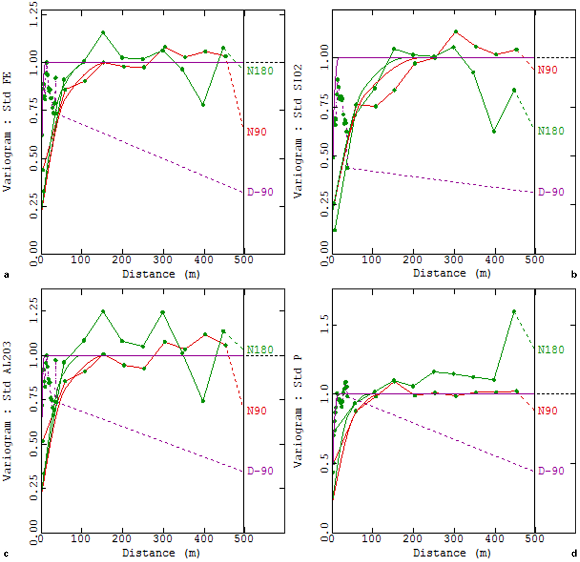
Semi-variogram models for iron, silica, alumina and phosphorus standardised to a variance of one for mineralised DG1
Estimation
Sixteen mineralised domains, based on the interpreted geology strands, are estimated using ordinary kriging (univariate) while 20 unmineralised domains are estimated using inverse distance to the power of one. Estimation is for the same 10 chemical variables and density as for variography. Cokriging is not used as there is no under-sampling of any of the variables to be estimated and so cokrigng is unlikely to produce better results than ordinary kriging and would take considerably more work (Journel and Huijbregts, 1978). The following steps are taken to ensure that the independent ordinary kriging of chemical variables does not cause undesirable artefacts:
direct variogram models have similar types of structure, ratios of nugget to total variance, types of structures, ratios of each structure to total variances and ranges of structures
the same kriging neighbourhood search is used for all estimates of chemical variables in the same domain
correlations and scatter plots of samples and estimated blocks are checked to see that they are approximately similar
total assay sums all 10 chemical variables with appropriate adjustment for oxide state. Total assay should be within 98 to 102% and blocks with total assay outside this limit are examined.
The estimation utilises the following options:
ordinary kriging is used
sample selection and block selection during estimation is based on the geozone code
hard boundaries are used for all domains
samples used for estimation meet a minimum length criterion
density is estimated independently of chemical variables and thus has its own search parameters
discretisation used is 5 m by 5 m by 2 m
sample selection is restricted to a maximum of four samples per hole
an octant based search is used in all runs with a maximum of 12 samples per octant
the minimum number of samples per estimate is generally 12, but decreases to four in the last run for some domains due to isolated pods of mineralisation
the maximum number of samples per estimate is 48
unfolding using the projection option in Vulcan is used for all mineralised domains except the hydrated domains and the detritals which have more horizontal orientations
parent cell estimation is used and this assigns the parent cell grade to sub-cells within the same geozone
drill hole samples which have manganese values above defined limits are not used for estimation of any of the chemical variables in blocks when the blocks are beyond specified distances from the drill hole samples. This restricts the distance of influence for manganese samples above the limits to reduce smearing of high sample values in the block model
blocks which are not estimated for chemical grades or density have the average geozone grade values assigned using scripts
small negative values produced in the estimation are substituted with detection limit values. A low number of small negative values are estimated for manganese, sulphur, titanium oxide and calcium oxide and these are due to negative kriging weights.
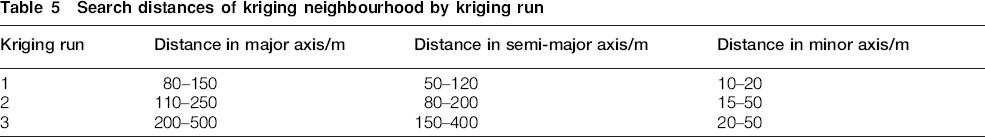
A kriging neighbourhood analysis is carried out for iron and density for the mineralised domains where there are enough samples to make such a study worthwhile. Kriging neighbourhood analysis domains are detritals, J2, J3, Joffre hydrated, Whaleback Shale Lower, Whaleback Shale Upper, DG1, DG2, DG3, Dales Gorge Hydrated and Footwall zone. Ordinary kriging uses three runs to interpolate grades for most domains. Two runs are used to estimate all variables in detritals and to estimate density in J5, DG1, DG2 and DG3. Two runs were used in these cases to avoid a high level of smearing of high values in the third run. Search parameters are used that ensure as many blocks as possible are estimated in the first run while attempting to keep the slope of regression close to a value of one and the number of negative kriging weights below 5%. Distances of the kriging neighbourhood are shown in Table 5 for each kriging run. Kriging neighbourhood analysis generally follows the methods proposed by Rivoirard (1987) and Vann et al. (1993).
Search distances of kriging neighbourhood by kriging run
Unfolding is used during estimation of most mineralised domains at BS4 to align the sample search with the folded beds. The projection model option in Vulcan is used to unfold samples and blocks. The projection model method can be used as bedding is not overturned. Lower and upper triangulation surfaces are used to guide the unfolding process. The projection model method is a vertical flattening which reassigns the Z (vertical) coordinate of samples and blocks so that the lower triangulation surface has an elevation of 0 in unfolded space, and the upper triangulation surface has an elevation of 1 in unfolded space. Samples and blocks do not have to lie between the surfaces, though they must lie within the X (easting) and Y (northing) extent of both surfaces. If samples or blocks are below the lower unfolding surface then they are given a Z coordinate of less than 0 in unfolded coordinates. Similarly, if samples or blocks are above the upper unfolding surface then they are given Z coordinates greater than 1 in unfolded coordinates. Samples and blocks are unfolded, then blocks are estimated and finally blocks are back-transformed to the original data space. With Vulcan software unfolding is carried out as part of the estimation process rather than being a separated data preparation step prior to estimation.
Validation and modelling checklist
Extensive validation is carried out on the estimated model using a standard series of checks. Visual validation of the block model is undertaken by comparing section slices of the block model against the drill hole interpretations and samples used to estimate grade into the blocks as shown in Fig. 6. Figure 6 shows that block grades visually match the adjacent drill holes. Unfolding is successful in orienting the search to lie along the bedding and produces a better estimate than using a search in real world Cartesian units.
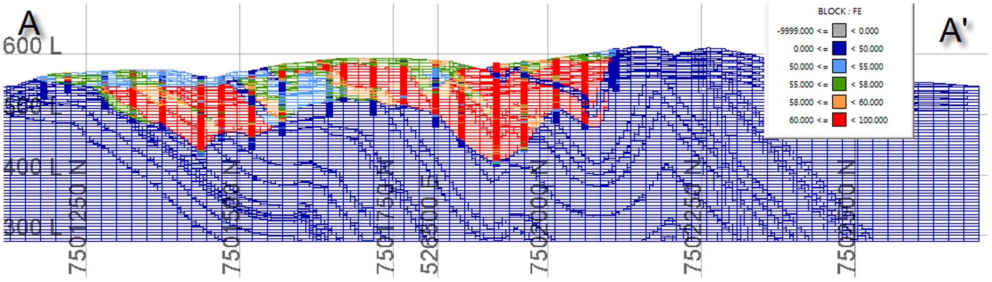
Typical cross-section of iron in drill holes and estimated block mode. Drill hole spacing is 50 m and the section is seen looking west
Statistical comparison is made between the average grade of samples and the average grades of estimated blocks for each domain. Comparison is made for both absolute and relative per cent differences. Relative per cent differences are small with the exception of some minor elements which often have a significant number of low values near the detection limit with occasional higher grade values, for example manganese oxide, sulphur, titanium oxide, magnesium oxide and calcium oxide.
Ordinary kriging estimates have unavoidable smoothing due to the goal in ordinary kriging of minimising the estimation error. High grade blocks tend to be underestimated and low grade blocks tend to be overestimated. A global change of support method is used to check whether the level of smoothing is acceptable. Change of support provides a theoretical global block distribution at the required block size estimated for the elements analysed and this theoretical distribution is compared against that of the estimated blocks. Global change of support only requires a declustered histogram of sample grades and a reliable semi-variogram model; a block model is not needed. Sample grades are transformed using a semi-variogram model from sample (point) support to block support. The global change of support suggests that the resource model is slightly conservative and underestimates the amount of high grade mineralisation and overestimates the amount of low grade mineralisation. The largest differences between the block model estimate and the global change of support are for the detrital, hydrated or more shale-rich strands. For most domains, the tonnes of high grade are within 10% of the anticipated global change of support value. Overall, the global estimate is within acceptable limits such that the model may be considered robust overall.
Sectional swaths plots are used to compare average grades of samples and average grades of blocks within rectangular panels of data within the deposit; and are generated separately for all domains, all chemical elements and density. Comparisons are made for cross section panels, long section panels, and vertical panels. The cross and long section panels are spaced at 100 m intervals, while the elevation panels are spaced at 5 m intervals. Graphs are produced and these show the tendency of the estimation to smooth out extreme values whilst matching the same broad grade trends as the average of samples within each drill line. The average grade data is taken from an evenly spaced corridor centred on the drill lines to account for samples off section. Figure 7 displays an example swath plot and has section slices made across strike for average grades of iron from samples and estimated blocks in the Dales Gorge 1 (DG1) unit. This domain has a high number of samples on most section slices. The average grades of samples are close to the average grades of blocks unless there are low numbers of samples. The average grades of blocks in swaths are smoother than the average grades of samples.
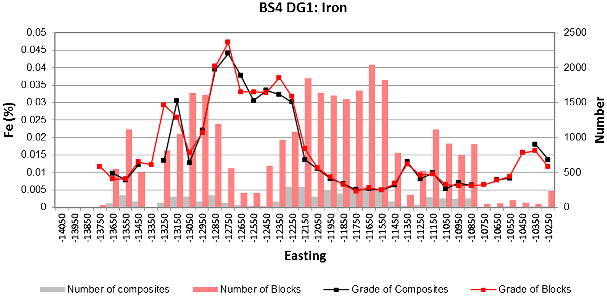
Validation swath plot of iron for the DG1 unit showing numbers and grades of samples and blocks by easting
Reconciliation
All models at operating sites including the BS4 model are reconciled against grade control data as part of the validation process.
The current BS4 block model is reconciled with the mine geology block outs which are based on blast hole samples. The mine geology block outs or dig plans can be regarded as the final mining model. Both the resource model (sub-blocked) and the reserve model (which may be reblocked) are reconciled versus mine geology block outs. The aims of these reconciliations are:
to support the Mineral Resource and Reserve Statement
to better understand the estimation and confirm the choices of estimation parameters
to support site use of the model
to understand and reconcile the impact re-blocking has on the Ore Reserve estimates
to identify the core drivers of non-performance in order to correctly target improvement options.
Factors are calculated to allow comparison between reconciliation at difference sites and time periods (Fouet et al., 2009). The two main factors for the resource model tonnes are:
R2 = (mine geology tonnes)/(resource model tonnes)
R3 = (mine geology tonnes)/(reserve model tonnes)
Similarly for grade, the two main factors for the resource model grade are:
R2 = (mine geology grade)/(resource model grade)
R3 = (mine geology grade)/(reserve model grade)
These factors are similar to the F1 factor of Parker (2012). Control limits are defined for tonnes and grades for R3 and investigations are made when reconciliations are outside the control limit, particularly if a consistent trend has been present for a number of quarters. Control limits are set after statistical analysis of historic reconciliation performance over quarterly mining periods and determination of what defines a significant reconciliation non-conformance. Factors are calculated for volume and tonnes of high grade, low grade and waste, density, and grades of iron, silica, alumina, phosphorus, and, in Marra Mamba deposits, manganese.
Reconciliations are made between the new block model and mine geology block outs as there is several years of historical mining at BS4. The block model is loaded to a Microsoft SQL Server database. Reconciliations are run using an internally developed reconciliation system which accesses the database of block models. As blasts are developed during mining, the blast solids and mine geology block outs (dig blocks) are also loaded to the database. The model is reconciled with production and reconciles better than the previous model as the new model is based on additional drilling information and an improved geological interpretation. Such new models need to demonstrate quantifiable improvements from the reconciliations before they are released.
Model review process
Internal peer review is undertaken to ensure the BS4 model is to a high standard and all modelling procedures are followed. The internal peer reviewer checks the following before the model undergoes a detailed review by the Competent Person and is released to users. The peer review process is ongoing as the model is made and covers:
the list of model stakeholders and whether they have been consulted during modelling
purpose and scope of the model
raw data quality and data sets
QA/QC of sampling and assaying
down hole data interpretation
geological model
validation
density data analysis
continuity analysis via variography
estimation parameters and kriging neighbourhood analysis
estimation parameters in the Vulcan block estimation file
resource classification and resource statement
model standardisation and reporting
loading of model to database for reporting and reconciliation
documentation, file housekeeping and close off.
In addition to internal peer reviews, which occur for all models, resource estimates are also subject to external audits. The group audit has been established by the Rio Tinto board as part of the corporate governance assurance program. The group audit process ensures all aspects of Public Reporting undergo independent expert audit and this includes the RTIO Mineral Resources and Ore Reserves.
Classification
While the JORC Code (JORC, 2012) provides the minimum standard for Mineral Resources, Rio Tinto has additional requirements prior to a Mineral Resource being published. At the heart of these additional requirements is the need to demonstrate that the project has a positive economic return, using long term pricing forecasts. To do this, initial mine designs incorporating geotechnical knowledge and metallurgical performance data are used to deliver a mine schedule. The schedule is then used by a business analyst, along with current operating cost and estimated capital costs (including sustaining capital), to derive a net present value for the deposit.
The classification process for Mineral Resources within RTIO uses all of the data and modelling work undertaken and detailed analysis of the key geological risks. In classifying the deposit, the Competent Person considers:
the nature and quality of the sampling and assaying including the spatial distribution of the drilling for different vintages of data
the nature, quality and amount of down hole gamma–gamma density data and quality of the correction factors to convert wet density values to dry bulk density equivalent
the style of mineralisation and the complexity of the geological structures controlling mineralisation or post mineralisation intrusions and its interrelationship with the drill spacing
the amount of inherent smoothing within the estimate with reference to the cut-off grade
the spatial distribution of the data relative to the estimated domain
the results of the model validation
the quality of the model when reconciled to grade control information for operation models.
Model progression
As multiple teams are involved in the estimation and use of resource models, a series of model progression meetings are arranged.
The first progression meeting occurs between members of the Resource Evaluation Division who undertake drilling and prepare the geological model, members of the Resource Geology Department who perform the estimate, site geologists, mining engineers and the Competent Persons. Data collection, data quality and geological risks are discussed.
The estimated sub-celled resource model is presented by the resource estimation geologist at a model handover meeting to model users including the Reserves Data Management Department, site geologists, mining engineers, metallurgists and study managers. The focus of the progression is the outcomes of the modelling work which is invariably customised to the deposit in question.
Resources
Mineral Resources for the BS4 Deposit, as at 31 December 2012, are estimated at 47 Mt at 62·3% Fe of Measured Resources, 13 Mt at 61·9% Fe of Indicated Resources and 3 Mt at 62·9% Fe of Inferred Resources, for a total of 63 Mt at 62·2% Fe. The Mineral Resources are stated as Mineral Resources in addition to Ore Reserves (a Rio Tinto policy) and represent dry metric tonnes. The Ore Reserves are estimated to be 422 Mt at 62·3% Fe Proved Reserves and 139 Mt at 61·3% Fe of Probable Reserves for a total Ore Reserve of 561 Mt at 62·0% Fe. Ore Reserves are dry metric tonnes of product.
Model and data storage
Upon model completion, modelling files are sorted, duplicate versions rationalised and the files are arranged in a standardised and regularised directory structure. This directory structure is common to most RTIO modelling projects and allows modelling files to be easily located later. The completed resource model is loaded to a SQL server database for resource reporting and reconciliation. The Vulcan sub-celled block model is provided to mine planning engineers to be regularised to a constant cell size which represents the selective mining unit. The regularised model is used for short term, medium term and long term mine planning, including use in Whittle and XPAC software.
Conclusions
Resource estimation of the BS4 deposit has been presented to show techniques that are sufficiently robust for mine planning and public reporting of a bedded iron ore deposit in the Pilbara region. Data collection, interpretation, modelling and estimation methods have been developed over many years. A spacing of 50 m by 50 m for RC drill holes is suitable for long term resource models of the BS4 deposit. Modelling requires that drill holes are logged by down hole geophysical methods, sampled at 2 m intervals, geologically logged and the samples assayed by XRF. Geological logging assigns samples to different domains and the domain number is stored in the drill hole database. Directional semi-variograms are needed for ordinary kriging and are modelled for each mineralised domain for iron, silica, alumina, phosphorus, manganese, LOI, sulphur, titanium oxide, calcium oxide and magnesium oxide, as well as density. Kriging neighbourhood analysis allows the search parameters to be optimised. Ordinary kriging is currently considered to be the most effective estimation method and incorporates unfolding with vertical flattening for mineralised domains, allowing the kriging sample search to effectively bend along bedding. Contact analysis supports the uses of hard boundaries for estimation. Estimation is done by domain and the block model is flagged for geological domains by using interpreted wireframes. Inverse distance estimation is used for waste domains. A centralised Microsoft SQL Server database stores resource models and allows more efficient reconciliation and resource reporting. Resources are classified according to the JORC code 2012 by the Competent Person for public reporting.
Footnotes
Acknowledgements
The support of Rio Tinto Iron Ore is gratefully acknowledged to provide the resources to prepare this paper and to allow the paper to be published. The techniques presented for data collection, estimation, validation and reconciliation are based on the work of many Rio Tinto geologists past and present. Dr M. Abzalov and two anonymous reviewers are thanked for their reviews of this paper. This paper is an expanded and revised version of the paper published in the monograph Mineral Resource and Ore Reserve Estimation -� The AusIMM Guide to Good Practice (Sommerville et al, 2014). Permission of the AusIMM to publish this revised paper in AES is gratefully acknowledged.