Comparative study of iron ore characterisation using a scanning electron microscope and optical image analysis

Abstract

In order to develop downstream processing routines for iron ore and to understand the behaviour of the ore during processing, extensive mineralogical characterisation is required. Microscopic analysis of polished sections is effective to determine mineral associations, mineral liberation and grain size distribution. There are two main imaging techniques used for the characterisation of iron ore, i.e. optical image analysis (OIA) and scanning electron microscopy (SEM). In this article, a QEMSCAN system is used as an example of SEM methodology and results obtained from it are compared against results obtained by the CSIRO Recognition3/Mineral3 OIA system. Both OIA and SEM systems have advantages and drawbacks. Even though the latest SEM systems can distinguish between major iron oxides and oxyhydroxides, it is still problematic for SEM systems to distinguish between iron ore minerals very close in oxygen content, e.g. hematite and hydrohematite, or between different types of goethite. Scanning electron microscopy systems also can misidentify minerals with close chemical composition, i.e. hematite as magnetite and vitreous goethite as hematite. In OIA, iron minerals with slight differences in their oxidation or hydration state are more easily and directly recognisable by correlation with their reflectivity. In both methods, the presence of microporosity can result in some misidentification, but in SEM methods misidentifications due to microporosity can be critical. Low resolution during QEMSCAN analysis can significantly affect the textural classification of particle sections. The main conclusion of this study is that, for low iron content ores or tailings, SEM systems can provide much more detailed information on the gangue minerals than OIA. However, for routine characterisation of iron ores with high iron content and containing a variety of iron oxides and oxyhydroxides, OIA is a faster, more cost effective and more reliable method of iron ore characterisation. A combined approach using both techniques will provide the most detailed understanding of iron ore samples being characterised.

Keywords

Optical image analysis QEMSCAN SEM Iron ore Characterisation Hematite Magnetite Porosity

Introduction

Quantitative mineralogical analysis is a valuable tool for ore quality evaluation and optimisation of metallurgical process performance; for instance, targeting grinding size based on liberation characteristics of valuable minerals. Traditionally, evaluation has been carried out by point counting under the optical microscope. This technique depends on careful calibration between experienced operators and is labour-intensive, but is well established and proven. Automated, computer-based image analysis systems are having increasing applications in mineralogical evaluation, as relatively low cost digital storage capacity and processing speed are becoming capable of handling volumes of very large, high-resolution images.

Currently, there are two main imaging techniques used for characterisation of iron ore, which involves specific challenges, described later in this paper. These are optical image analysis (OIA) and scanning electron microscopy (SEM). One of the advantages of computer-based OIA systems is their significantly lower capital and maintenance cost. In this paper a QEMSCAN system has been used as an example of SEM methodology (Gottlieb et al., 2000) whereas the OIA system Recognition3/Mineral3 developed at CSIRO (Donskoi et al., 2010, 2013) is used as an example of a current optical-based system.

In SEM-based systems, the sample is scanned by the electron beam and the system identifies different minerals using X-ray spectra and backscattered electron (BSE) signals that are emitted from the sample (Gottlieb et al., 2000). Whereas QEMSCAN maps the whole surface of particles, collecting energy-dispersive X-ray spectra across a grid with user-defined resolution, the Mineral Liberation Analyser (MLA) depends on segmentation of regions based on BSE brightness, followed by energy-dispersive X-ray analysis of single geometric centre points, or mapping across a grid (Figueroa et al., 2011).

In OIA, each sample (usually one size fraction) is mounted in an epoxy resin block, which is polished on one side, imaged under reflected, plane polarised light and analysed (Danti et al., 1993; Gomes et al., 2010; Iglesias et al., 2011). The recognition of different minerals is based on the reflecting power of the surface (reflectance) of the minerals examined. This can become a limitation if different minerals have similar reflectivities. Older OIA systems [Zeiss KS400 or VideoPro (Danti et al., 1993) for example] had only 255 gradations in grey scale (or selected Red, Blue or Green channels), which was sometimes not enough to distinguish between even visually different minerals (Bonifazi, 1995). In comparison, modern systems like the Zeiss AxioVision (AxioVision 2006–2009) system have more than 16 000 levels of intensity, so even differences invisible to the human eye can be easily recognised.

Significant improvements in camera sensitivities have also provided a partial solution to the OIA problem of distinguishing non-opaque minerals from epoxy mounting resin. Minerals like apatite, amphibole, calcite and garnet are now recognisable with OIA (Lane et al., 2008). On the other hand, reliable OIA-based automatic identification of quartz within epoxy is still an issue. However, significant progress has been made recently (Poliakov and Donskoi, 2014). CSIRO has developed a method for automatic quartz segmentation based on relief produced by quartz during polishing of the resin block. Figure 1 shows three images: the first is an optical image of an oxidised/hydrated manganese ore sample, which has significant quartz content. The second image has been enhanced for quartz identification, whereas the third is the mineral map of the sample, where automatically identified quartz particles can be seen (cyan colour). This method correctly identified 90–95% of quartz in this particular sample. Due to the large amount of quartz present, the relative error is quite small. For smaller amounts of quartz and for other ores, the error can be higher. CSIRO is currently working on improvements to this method. Two other methods of quartz identification are being worked on concurrently with this method. The first is based on the idea of using epoxy with a specially created texture, so the problematic non-opaque mineral areas can be identified by the distortion of texture in the resin underneath the non-opaque mineral. The other idea is to use the bireflectance of problematic non-opaque minerals.

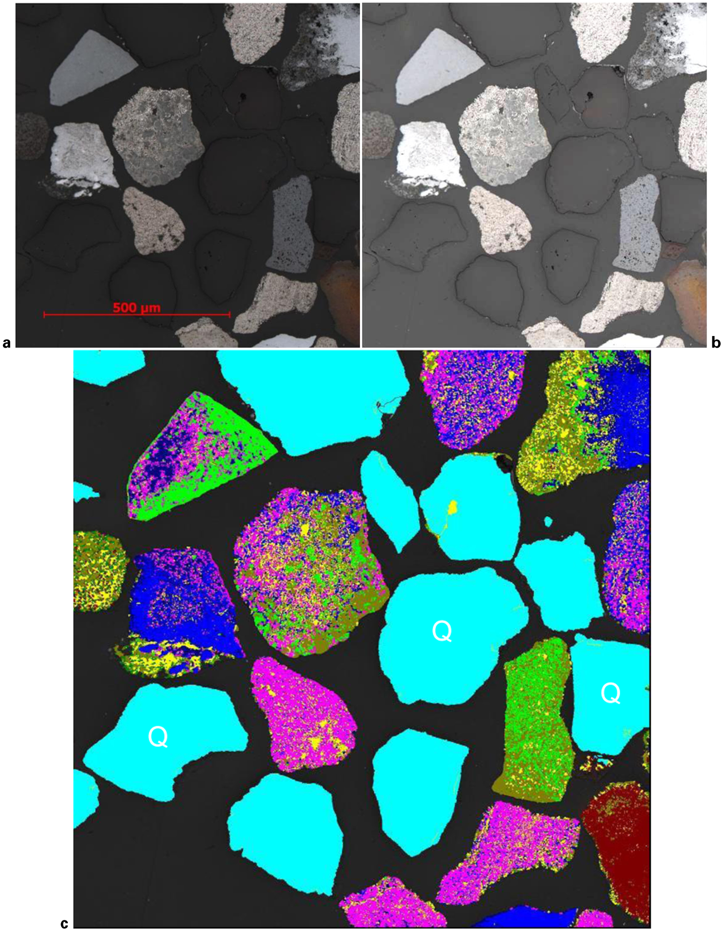
a ore photomicrograph; b image enhanced for quartz automatic identification; c coloured mineral map (Q = quartz, cyan)

Correlation with mineral reflectivity allows recognition using OIA of iron minerals with very slight differences in oxidation or hydration. The higher the hydration level of an iron oxyhydroxide, the lower is its reflectivity, and so the darker it appears in a photomicrograph (see Fig. 3). For example, it is very important to be able to distinguish between hematite and hydrohematite as even small amounts of hydrohematite can result in significant lump ore decrepitation within the blast furnace, and significant changes in sintering reactivity compared with hematite. The potential for explosive decrepitation of hydrated iron oxides has been long known (Spencer, 1919).

Relatively recent advances in X-ray acquisition and processing capability have enabled the development of methods to identify major iron oxides and hydroxides using SEM technology (Maddren et al., 2007; Figueroa et al., 2011). The development of an iron ore characterisation capability was an important breakthrough in SEM technology and required several novel approaches. The first was the use of an eAMP backscatter amplifier, which was placed between the backscattered electron diode detector and the Pre-Amplifier. It is vital for the analysis of iron ore to significantly improve BSE signal stability, in order to maintain accurate discrimination based on the very small differences in Fe∶O ratio between major iron oxide mineral phases. The eAMP has a fixed gain and offset, which is unaffected by the brightness and contrast settings on the SEM and is insensitive to temperature fluctuations. The second significant development was a change in calibration procedure. For iron ore characterisation, a 3-point backscattered electron (BSE) calibration should be used (e.g. gold, quartz and copper standards) instead of a 2-point calibration (gold, quartz). This is done in order to maintain a more stable BSE signal versus average atomic number curve on a SEM system and between SEM systems. The third development was a new species identification protocol, an algorithm for identifying major iron ore minerals.

These developments provided a great opportunity to simultaneously identify gangue, and iron oxides and hydroxides within iron ore, together with their associations. However, certain limitations of the QEMSCAN method still remain. The main limitation is resolution. The calculated resolution of OIA systems in air is around 0·30 μm (better in oil) although the best possible resolution that can be achieved with an optical microscope is even lower at about 0·2 μm (Slayter, 1998). The ideal resolution of QEMSCAN is determined by the electron beam excitation volume, which for primary X-ray emission can be very small, but for typical measurements is from 0·5 to 5 μm (linear size) for solid structures. For porous structures it can be higher. However, this is not the only resolution-limiting factor. Due to the point-by-point technique, small distances between consecutive measurements result in extremely high overall imaging times. For typical QEMSCAN characterisation, the distance between measurements is 5–10 μm. The majority of Australian iron ores have very complex textures (Beukes et al., 2008; Clout, 2003; Clout and Simonson, 2005; Donskoi et al., 2005, 2008b, 2010; Morris, 1980) and textural information itself is very important for downstream processing prediction (Clout, 2003; Donskoi et al., 2006, 2007, 2008a, 2008c; Zhang and Subasinghe, 2013), where texture is defined here as the spatial distribution of different minerals (many authors prefer the term ‘fabric structure’). A resolution of 5–10 μm is not sufficient to correctly identify and classify different textures in the majority of Australian iron ores.

It is often important for iron ore characterisation to distinguish between two different textural types of hematite, e.g. martite and microplaty hematite. From the image processing point of view, this is also a difficult task and even experienced mineralogists cannot always make the distinction with confidence. However, for some ores automated identification of the two types of hematite is quite feasible. An example of the CSIRO OIA system making such identification is provided in Fig. 2.

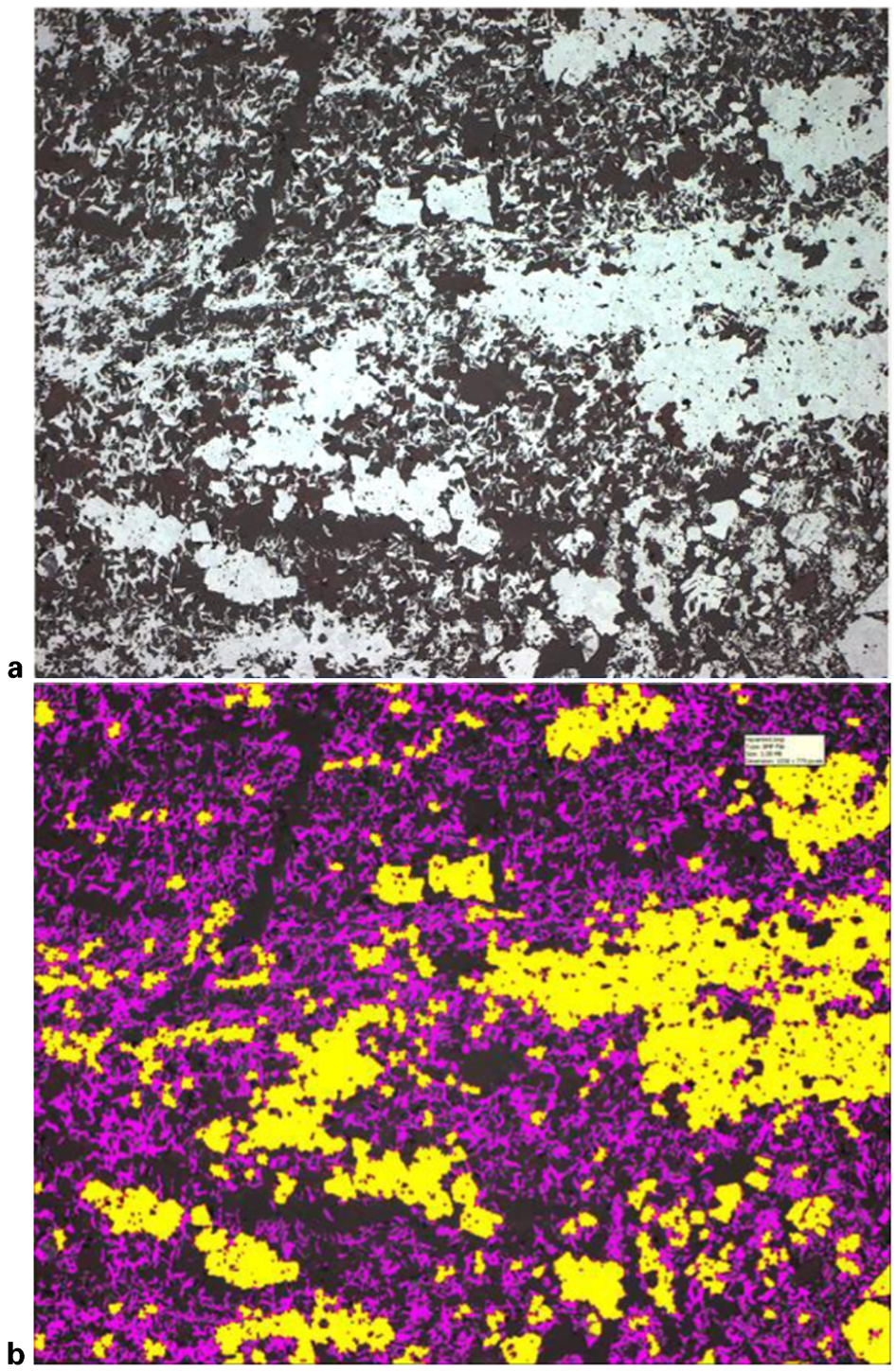
a original optical photomicrograph; b mineral map (martite is yellow, microplaty hematite is magenta)

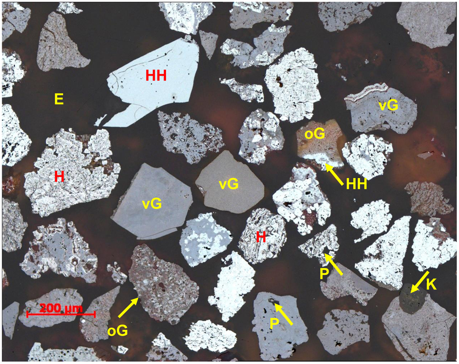
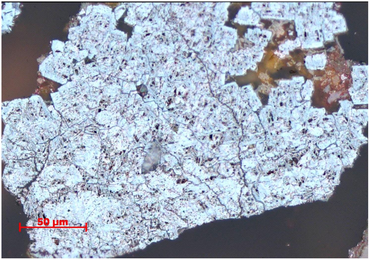
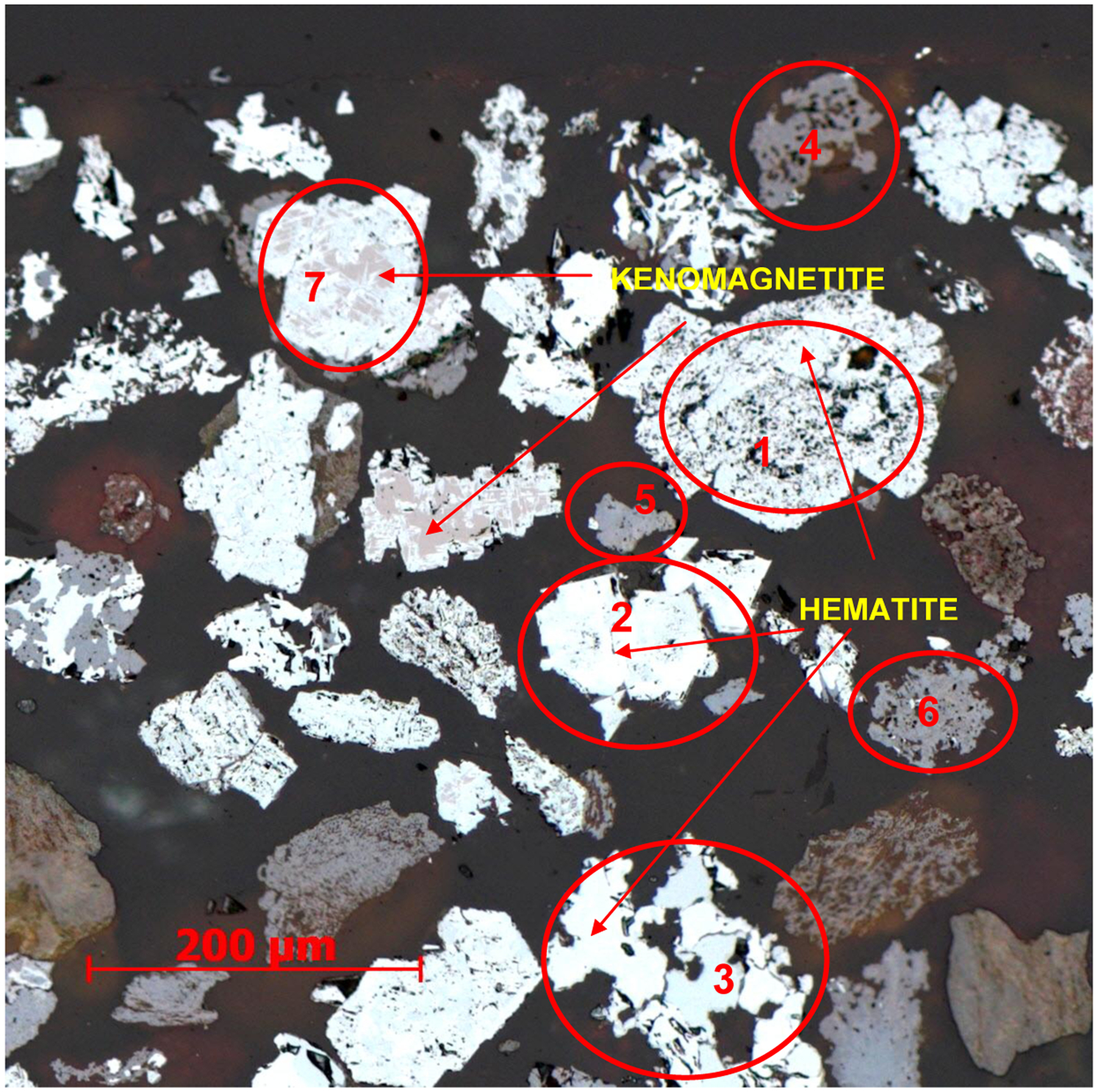
Reflected light optical photomicrograph of a polished block for sample RM (200×) (Marra Mamba fine ore, size fraction −250+150 μm). H = hematite (martite), HH = hydrohematite, vG = vitreous goethite, oG = ochreous goethite, K = kaolinite, P = pore, E = epoxy resin

Among other limitations of SEM is its inability to distinguish between different minerals with the same chemical composition and with similar backscatter signal, and to distinguish between different grains or crystals of the same mineral. In OIA, different grain/crystal orientations can result in significant differences in reflectivity (Pirard, 2007). However, OIA has similar limitations when optical reflectivities of different substances are the same or significantly overlapping.

In this paper, the results for characterisation of two samples (RM and BM) of Australian iron ore by OIA and QEMSCAN are compared. Both samples are Pilbara hematite-goethite sinter fines. RM is a typical Marra Mamba fine ore, whereas BM is a Brockman fine ore with the addition of martite/kenomagnetite ore.

Analysis of sample RM (Marra Mamba fine ore)

A photomicrograph of a polished block prepared from sample RM is taken using the MosaiX technique (MosaiX is an AxioVision module; Fig. 3); which allows several individual images to be merged into one high resolution composite image. In this example, a 2×2 matrix was used, but it is possible to collect a much larger matrix of images (up to a 10×10 image matrix has been used by CSIRO) with a maximum image file size of 500 MB. The image in Fig. 3 was obtained under magnification 200× [0·5315 μm/pixel and numerical aperture (NA) 0·5], which corresponds approximately to an optical resolution of 0·55 μm in the visible spectrum, depending on the wavelength. The dimensions of this image are 2534×2006 pixels, and collection of one image like this typically takes 25 to 27 seconds.

Another image of approximately the same area (there is a small rotation) was obtained by QEMSCAN (Fig. 4) with 0·73 μm pixel spacing; its size is 1920×1440 pixels and it took over 3 h (184 min) to acquire. Increasing the pixel spacing to 1·5 μm would have decreased the acquisition time to around 45 min.

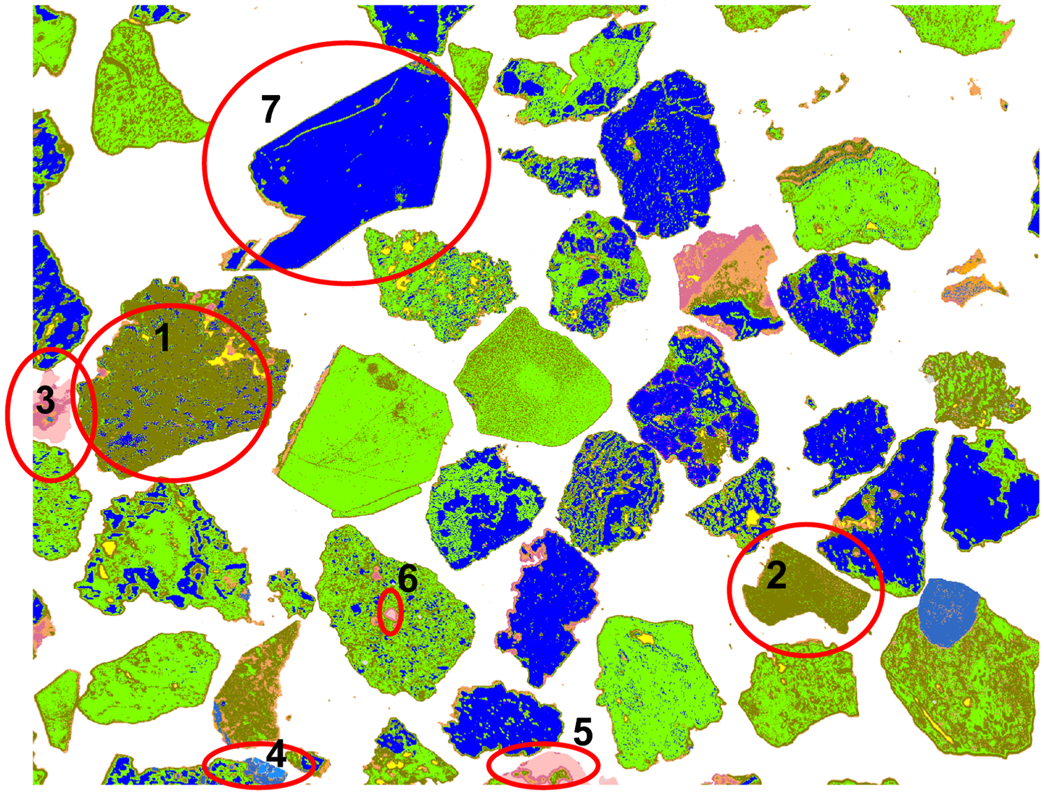
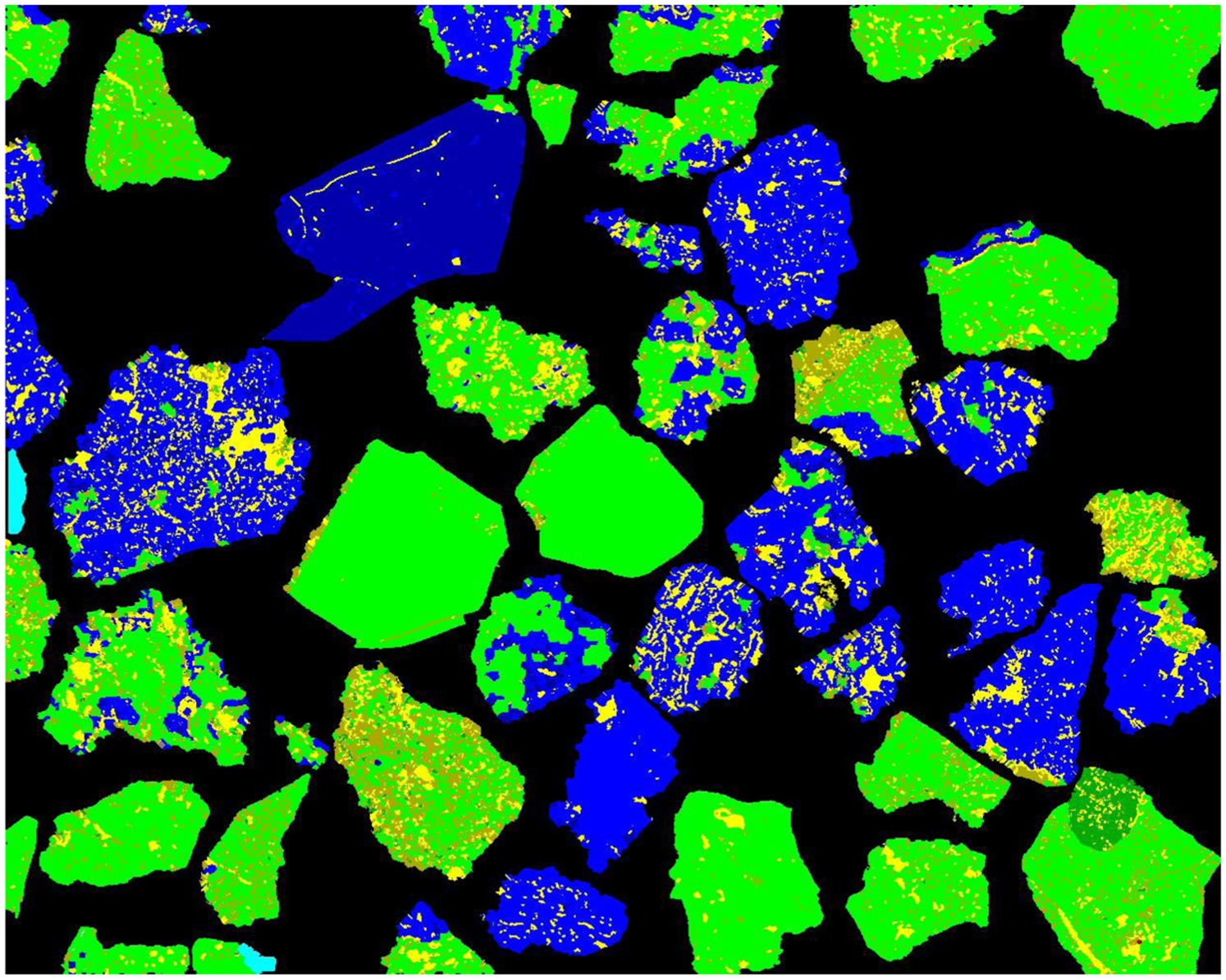
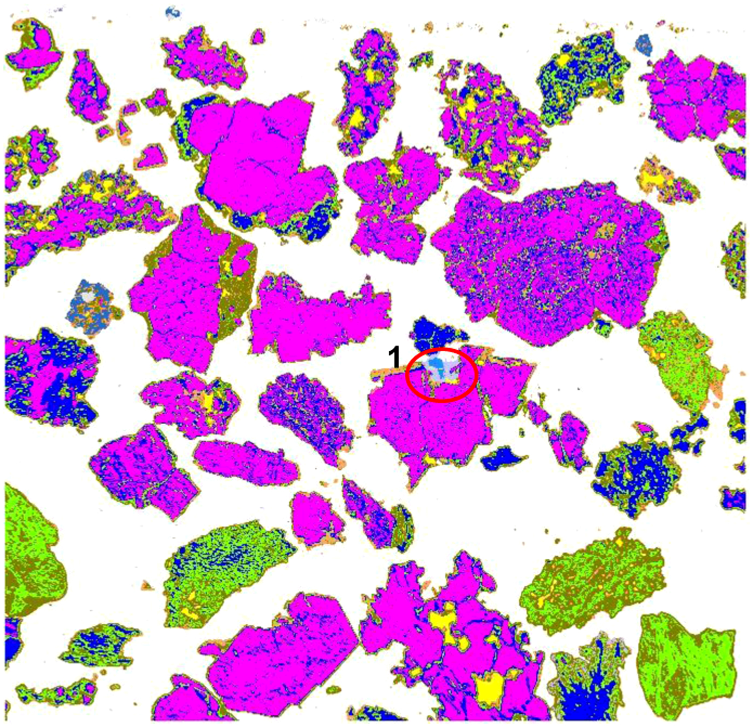
Image of the same area as in Fig. 3 obtained by QEMSCAN. See colour coding for mineral identification on Fig. 6 and text for explanation of the numbered areas

The mineral colour map (Fig. 5) was generated from the image shown in Fig. 3 with the CSIRO Recognition3/Mineral3 optical image analysis package (Donskoi et al., 2010, 2013). The QEMSCAN and OIA colour coding for different minerals is provided in Fig. 6.

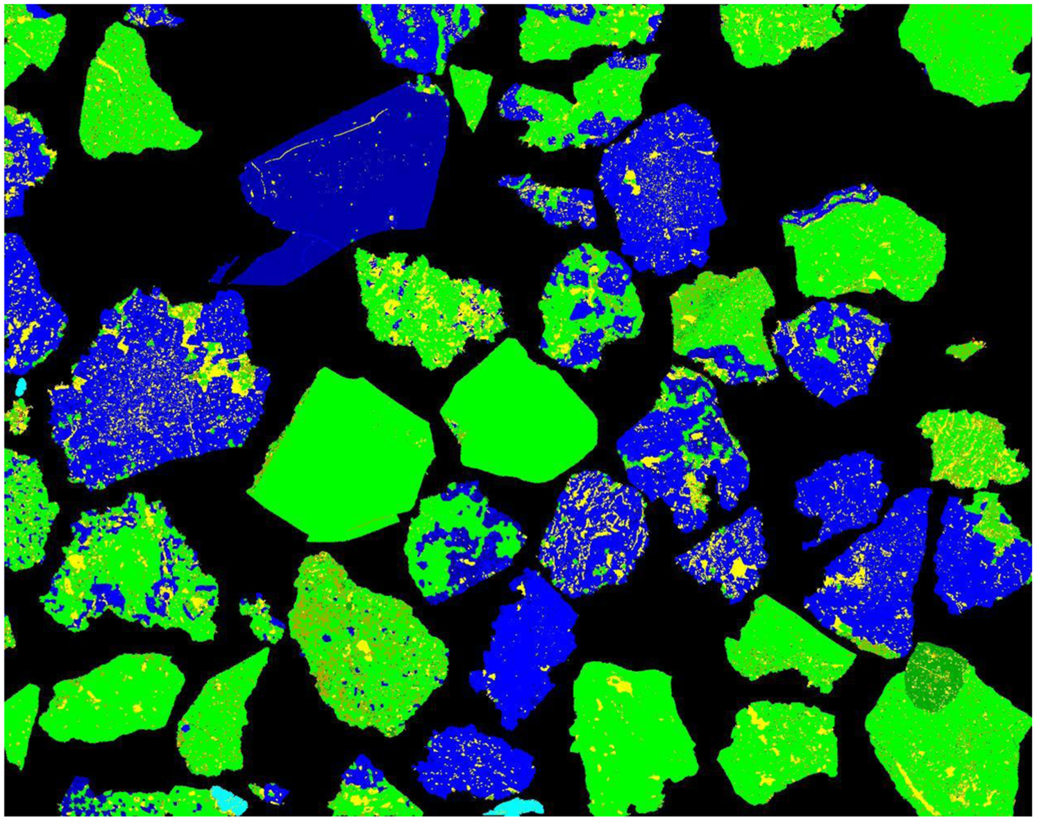
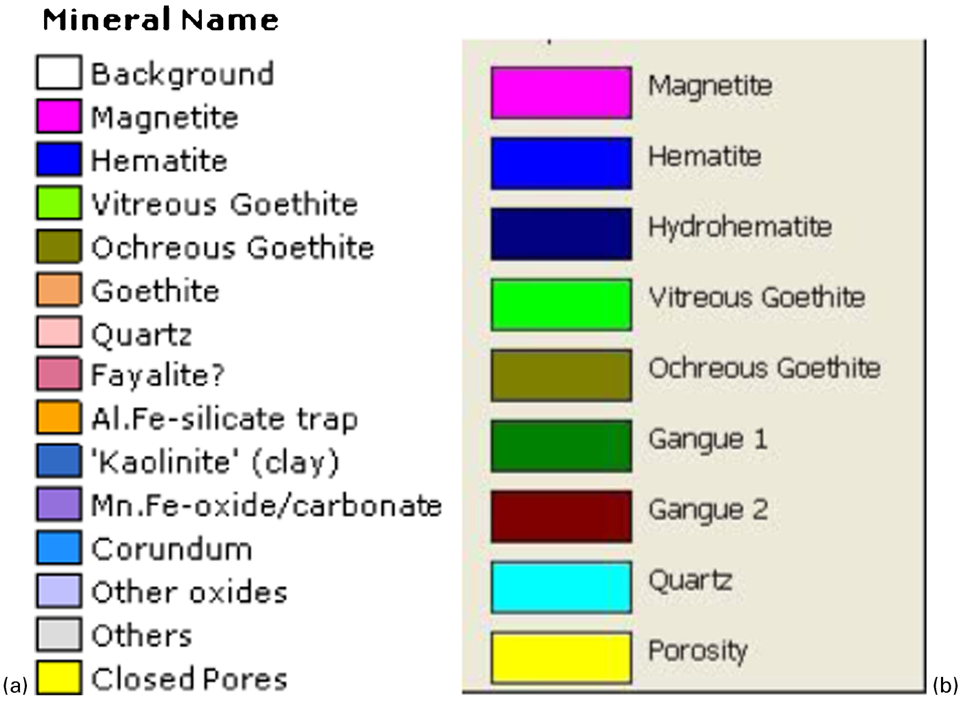
Mineral colour map obtained from the image in Fig. 3 (200×) with the CSIRO optical image analysis package Recognition3/Mineral3 (See colour coding for mineral identification on Fig. 6)

a SEM; b OIA (Gangue 1 – kaolinite, Gangue 2 – other gangue apart from non-opaque minerals, quartz – all non-opaque minerals)

Image processing can take different amounts of time depending on how complex, and therefore how precise, the operator wants the processing to be. Utilising an automated quartz identification procedure, the creation of the mineral map took 5 min 10 s (note that this procedure is still under development and has not yet been fully optimised). Without automated quartz identification, creation of the mineral map took 1 min 45 s. Further measurement of mineral abundances, perimeters, shape factors and other textural information for every particle took another 3 min 50 s (47 large particles altogether, with smaller particles removed to reduce stereological error).

In fact, the image parameters (high magnification and MosaiX) were chosen for comparison with SEM at similar resolution. There was no practical need to process the image at this magnification and it should be kept in mind that the relationship between processing time and image size is not linear. Another image of this area was taken with magnification 100× (1·0636 μm/pixel, NA 0·25), which corresponds approximately to an optical resolution of 1·1 μm in the visible spectrum. The image is very similar to Fig. 3. The size of the image is 1247×995 pixels and collection of a single image typically takes 5–7 s (2–3 s in the most recent Zeiss system). Processing with automated quartz identification took 45 s, whereas without quartz identification it took 15 s. Measurement for 47 particles took 1 min 7 s. The OIA mineral map obtained from the 100× magnification image (Fig. 7) is similar to Fig. 5.

Mineral colour map obtained using optical image analysis for the same area as the image in Fig. 3, but acquired at 100× magnification. (See colour coding for mineral identification on Fig. 6)

The first issue that needs to be discussed is the very strong edge effect present in the SEM image. Three areas from the QEMSCAN image in Fig. 4 are enlarged (Fig. 8). Almost every particle in these images has a thick edge of a mineral different from that present within the main particle area. Visual examination of these edges under the optical microscope at high magnification did not show any difference in mineralogy between the edge and the adjoining particle areas (see Fig. 3). The problem is probably caused by surface penetration of the electron beam at the edges of particles and pores such that the excitation volume is not fully within the same phase. It can be seen that the thickness and composition of the misidentified edge changes along particle boundaries and in some cases the edge effect is completely absent. Variation in this edge effect most likely depends on the inclination of the particle surface under the surface of the epoxy (see Fig. 9). Software correction for this phenomenon, which is available within the QEMSCAN software, can correct for boundary areas. However, this was not used for this work, because the technique requires pixel spacing equal to or greater than the electron interaction volume, which was not the case.

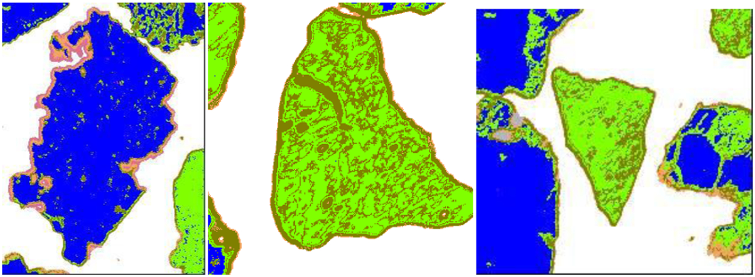
Edge effects during QEMSCAN identification

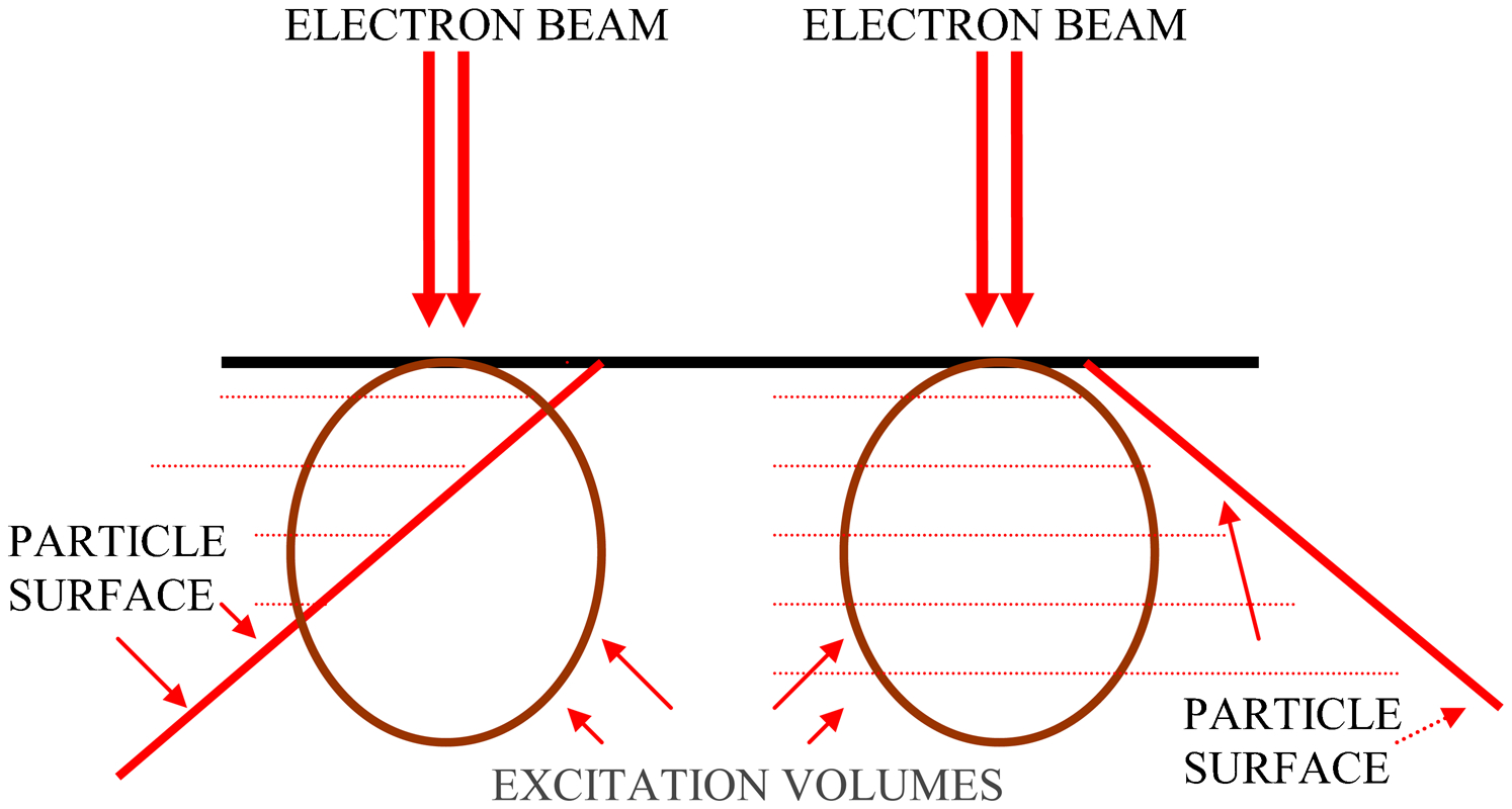
Dependence of excitation volume on particle surface inclination. (Left) only part of the excitation volume is within the mineral on the surface; (Right) excitation volume is fully within the mineral at the surface

A number of elliptical areas are marked in Fig. 4 and all particles or particle areas within these ellipses have some misidentification either in the SEM image or in OIA. These cases are discussed below.

The particle in area 1 is a microporous hematitic (martite) particle, except for the small porous area at the right-top which includes some gangue, vitreous and ochreous goethite. The latter can be seen more clearly in the high magnification (500×) image of this particle (Fig. 10). Due to the high and very finely distributed microporosity present in this particle, SEM identified the bulk of this particle as ochreous goethite, with only small, less porous areas identified as hematite and vitreous goethite. The porosity reduces the total Fe counts and backscatter signal leading to identification of the hematite as goethite (which has lower Fe and backscatter level than hematite/martite).

Hematitic particle from area 1 in Fig. 4 (magnification 500×)

Interference from the porosity also affected the optical reflectivity of this particle. Some small areas within this particle were identified as vitreous goethite (Fig. 5). However, the bulk of this particle was identified correctly by OIA as hematite.

The same effect is seen for the particle in area 2. Visual examination suggests that the bulk of this particle is porous vitreous goethite. Scanning electron microscopy identified the bulk of this particle as ochreous goethite. OIA also showed some presence of ochreous goethite, but the bulk was correctly identified as vitreous goethite.

In areas 3, 4, and 5, non-opaque minerals are present. Scanning electron microscopy identified these as quartz (3 and 5) and corundum (4). Traditional OIA would not recognise these areas at all, due to the overlap of their reflectance ranges with that of epoxy resin. The novel procedure for identification of non-opaque minerals, which is still under development, partially identified these areas (areas 4 and 5 under magnification 200×; areas 3 and 4 under magnification 100×), although OIA could not distinguish between quartz and corundum (note the mineral identified by SEM as corundum is likely to be gibbsite, however, SEM cannot detect water of hydration).

In area 6, a small quartz inclusion in a goethitic particle can be seen. Scanning electron microscopy identified it correctly. Correct identification of this area is also possible under the optical microscope, but during automated OIA such areas are usually identified as porosity, as can be seen in Figs. 5 and 7.

In area 7, a particle of hydrohematite was present and the chemical composition and BSE reflectance of hydrohematite and hematite are very close. Scanning electron microscopy cannot resolve this difference, and the current species identification protocol does not have any capability of distinguishing between hematite and hydrohematite. However, the difference in reflectivity between hematite and hydrohematite is recognisable by OIA. Using OIA analysis, this particle was identified as hydrohematite and it is correctly represented by dark blue (Figs. 5 and 7; hematite is lighter blue).

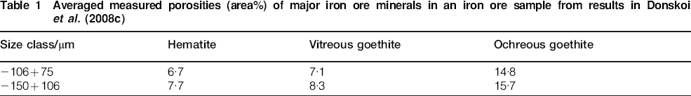
Correct identification of porosity is very important for calculation of mineral abundances, densities and all other related parameters. Different minerals have different average porosity values, some of which are dependent on the source/deposit. Data measured by Donskoi et al. (2008c) for major iron ore minerals in an iron ore sample are provided in Table 1. Quartz and magnetite usually have very low porosity. If porosity is not identified correctly, mineral abundance data can be significantly biased. Both SEM and OIA methods can identify some porosity (Figs. 4 and 6). However, SEM can only identify larger pores, even with the small step size used to produce the image in Fig. 4. Alternatively, OIA can identify much smaller pores (see Fig. 5) and the total area of this microporosity can be very significant (up to 50 or 60%).

Table 1

Averaged measured porosities (area%) of major iron ore minerals in an iron ore sample from results in Donskoi et al. (2008c)

Size class/μm	Hematite	Vitreous goethite	Ochreous goethite
−106+75	6·7	7·1	14·8
−150+106	7·7	8·3	15·7

Bulk mineralogical analysis by QEMSCAN can be achieved relatively rapidly with low resolution scans (10 μm pixel spacing or greater). This limits the analysis of texture and the analysis of complex fine structures such as those found in microporous martite-goethite ores. Part of a low resolution QEMSCAN report on samples RM and BM shows that low resolution can significantly restrict ore textural classification (Fig. 11). Porosity, grain size and textural peculiarities cannot be recognised. In comparison, OIA analysis routinely deals with images similar to the one represented in Fig. 3. High resolution allows very comprehensive automated ore textural classification to be performed (Donskoi et al., 2013).

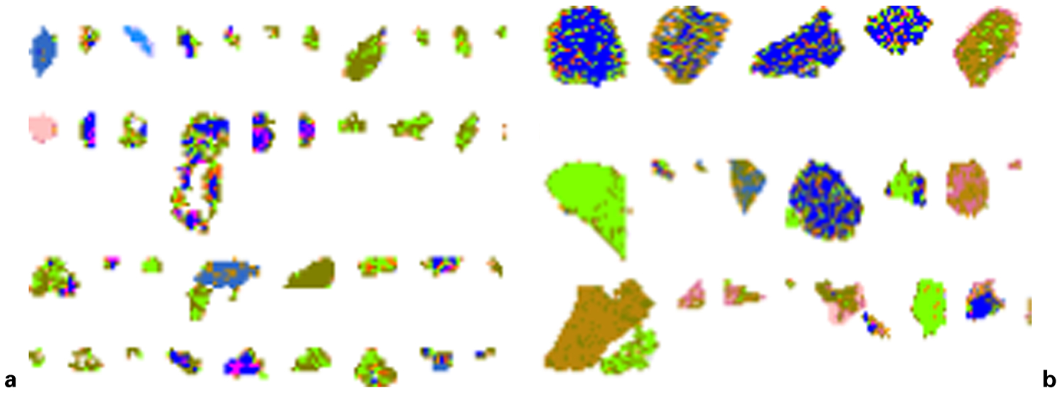
Examples of QEMSCAN reports on samples a BM and b RM

X-ray fluorescence (XRF) chemical analysis provides routine and reliable evaluation of exploration and production iron ore samples, but provides only limited, indirect information about mineralogy. Recent developments in the analysis of X-ray diffraction (XRD) data (König, 2013) demonstrate the potential value of XRD data in iron ore grade control. X-ray diffraction can provide information on mineralogy, but not texture, however, which is critical to the characterisation of texturally complex iron ores and understanding of lump and fine ore blend properties.

Both samples studied in this work were sent for XRD and XRF chemical analysis for reconciliation of the results obtained from OIA and SEM. X-ray diffraction data was recorded with a PANalytical X'Pert Pro Multi-purpose Diffractometer. Fe filtered Co K_α radiation, automatic divergence slit, 2° anti-scatter slit and fast X'Celerator Si strip detector were used for XRD data collection.

X-ray diffraction, SEM and OIA results for the sample RM are given in Table 2. For OIA, two sets of data are provided, which were obtained from composite images acquired with different objective magnifications. In the SEM results, together with data on ochreous and vitreous goethite, additional data on an intermediate goethite category is provided. To calculate mass abundances from area (volume) measurements, the same densities were used for the same minerals identified by both SEM and OIA.

Table 2

Mineral abundances in sample RM obtained from XRD, QEMSCANTM^TM and OIA

Mineral/mass%	XRD/%	QEMSCAN^TM	OIA (200×)	OIA (100×)
Magnetite	0·0	0·08
Hematite+hydrohematite	52·8	35·79	46·69	50·1
Hematite+hydrohematite	52·8	35·79	45·23+1·46	48·67+1·43
Vitreous goethite+ochreous goethite	44·4	58·94	50·64	47·56
Vitreous goethite+ochreous goethite	44·4	31·40+20·00+7·54	45·28+5·36	43·08+4·48
Kaolinite	1·1	0·98	1·76	1·84
Quartz+corundum	1·6	0·64	0·91	0·51
Quartz+corundum	1·6	0·63+0·01
Other		3·57
Porosity/vol.-%		0	10·02	9·54

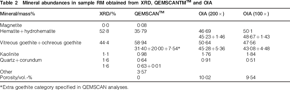
Extra goethite category specified in QEMSCAN analyses.

First, note that the amount of hematite in sample RM is overestimated by XRD (Table 2). A typical Marra Mamba ore with mineral abundances corresponding to the XRD measurements for sample RM should have a total iron content in the range 62–63% Fe, which does not match the chemical composition provided by XRF in Table 3 below, i.e. 60·68% Fe. The chemical composition provided by XRF should be the most reliable reference (although in exceptional cases, some XRF results for representative sub-splits of the same sample differ in total iron by up to 1·4% Fe). Scanning electron microscopy identified ∼5% non-ferrous material in this ore sample, whereas the XRD results indicate that only 2·7% non-ferrous material is present. Hence, the actual mineral composition appears to have less hematite and more goethite and gangue than XRD results are showing.

Table 3

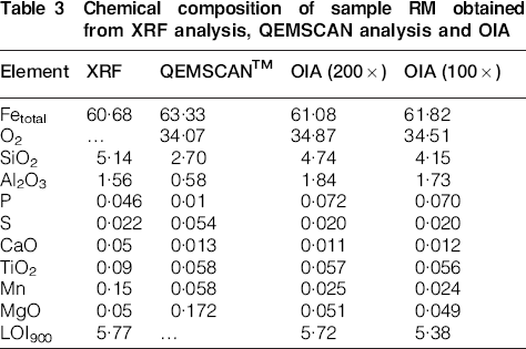
Chemical composition of sample RM obtained from XRF analysis, QEMSCAN analysis and OIA

Element	XRF	QEMSCAN^TM	OIA (200×)	OIA (100×)
Fe_total	60·68	63·33	61·08	61·82
O₂	…	34·07	34·87	34·51
SiO₂	5·14	2·70	4·74	4·15
Al₂O₃	1·56	0·58	1·84	1·73
P	0·046	0·01	0·072	0·070
S	0·022	0·054	0·020	0·020
CaO	0·05	0·013	0·011	0·012
TiO₂	0·09	0·058	0·057	0·056
Mn	0·15	0·058	0·025	0·024
MgO	0·05	0·172	0·051	0·049
LOI₉₀₀	5·77	…	5·72	5·38

The edge and other effects described for areas 1 and 2 in Fig. 4 (misidentification of porous hematite and vitreous goethite as ochreous goethite by SEM) have significantly reduced the proportion of hematite identified by SEM while significantly increasing the proportion of ochreous goethite (Table 2). The corresponding association and liberation data would also be significantly biased.

The data on chemical composition obtained by XRF, SEM and OIA for sample RM are presented in Table 3. To obtain such data using OIA, electron microprobe analysis is performed for a representative set of points across the minerals identified in the sample. Subsequently, microprobe data corresponding to the same mineral are averaged and entered into the CSIRO Recognition3/Mineral3 software. Based on calculated mineral abundances and microprobe data, the chemical composition of the whole sample is then calculated.

The highest total iron value was obtained by SEM analysis while simultaneously recording the lowest amount of hematite and the highest gangue content (Table 3). Optical image analysis reconciliation resulted in a slight overestimation of total iron relative to XRF analysis and good agreement of calculated and measured LOI. Silica was slightly underestimated by OIA, relative to XRF analysis, whereas alumina was slightly overestimated.

Analysis of sample BM

An optical photomicrograph of a polished section of sample BM was also obtained using the MosaiX procedure (2×2 matrix, magnification 200×; Fig. 12). The dimensions of this image are 1233×1228 pixels, which is bigger than a standard AxioVision image (1300×1030). The initial MosaiX image was 2533×2008 pixels, which was then cropped.

Reflected light optical photomicrograph of a polished block from sample BM (200×) (Brockman fine ore with the addition of martite/kenomagnetite ore, size fraction −150+106 μm). See text for explanation of the marked areas

Areas of kenomagnetite (pinkish) and hematite (white) can be easily discriminated in this image, and were confirmed by probe analysis. The difference in Fe∶O ratio between these minerals is small (average iron content from probe analysis for the hematite was 68·6% Fe and for the kenomagnetite 70·4% Fe). However, the presence of kenomagnetite can significantly affect processing behaviour (e.g. due to differing magnetic susceptibility) and reactivity.

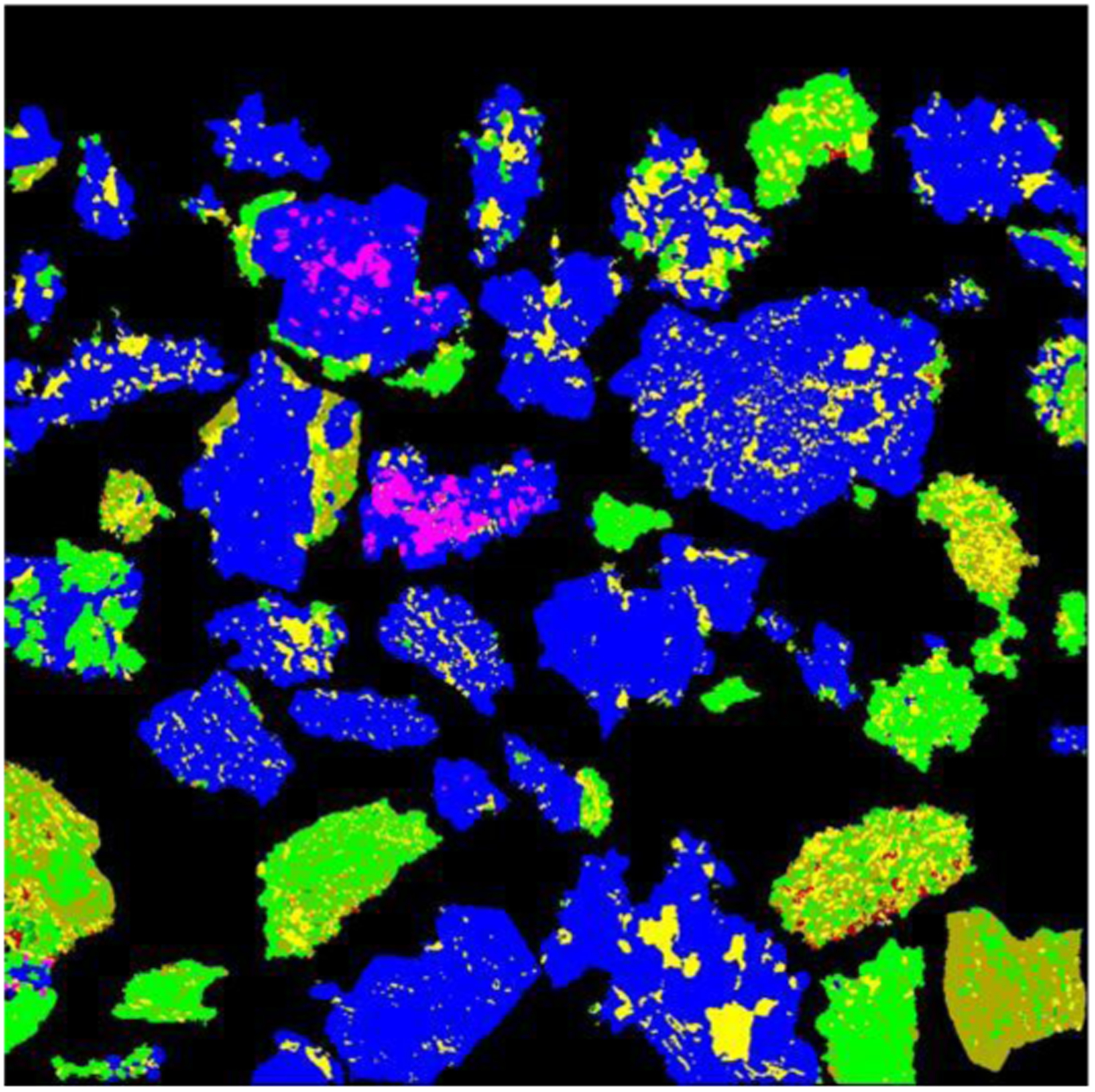
A processed image of approximately the same area obtained from SEM (Fig. 13) was collected with 1·00 μm pixel spacing; its size is 677×677 pixels and the time to collect it was 23 min (see Fig. 6 for colour coding).

Image of the same area as in Figure 12 obtained by QEMSCAN^TM. Marked area (1) shows possible gibbsite (identified by QEMSCAN^TM as corundum), (See colour coding for mineral identification on Figure 6)

Visual inspection of the particles in areas 1–3 (Fig. 12) does not show any presence of kenomagnetite. However, SEM identified these areas as magnetite. Rechecking showed that the backscatter intensity values from hematite in sample RM were around 86 (arbitrary units), whereas the backscatter values from hematite in sample BM were much higher at about 93·5 – right in the middle of the magnetite range. A possible explanation for this is that oxidation of magnetite to martite and formation of hematite during ore genesis may have resulted in differences in crystalline structure and composition of the hematite in the RM and BM samples that are reflected in backscatter intensity. A new version of the QEMSCAN spectral analysis engine was recently released that takes the entire spectrum into consideration, not just regions of interest corresponding to individual elements. Improved spectral analysis may resolve the issue and this matter will need extra investigation.

In areas 4–6 in Fig. 12, vitreous goethite particles are present (obvious grey colour in Fig. 12). However, SEM identified them as predominantly hematitic particles, although this did not happen for sample RM. It is probable that the nature of this misidentification is similar as for hematite particles, i.e. overlapping backscatter intensity ranges for hematite and vitreous goethite.

The mineral colour map obtained by OIA from the original image in Fig. 12 is shown in Fig. 14. As can be seen, the majority of the minerals are identified correctly, with the exception of the non-opaque minerals in area 1 (Fig. 13). Some small details of magnetite identification (e.g. the particle in area 7, Fig. 12) have also been lost. This happens due to the reflectivity overlap between magnetite, hydrohematite and vitreous goethite.

Mineral colour map obtained from the image in Fig. 12 (200×) using the CSIRO optical image analysis package Recognition3/Mineral3. (See colour coding for mineral identification on Fig. 6)

X-ray diffraction, SEM and OIA mineral abundance results for sample BM (Table 4) indicate that the XRD and OIA results are quite similar. However, SEM has significantly overestimated the proportion of goethite, so the combined magnetite and hematite value (56·41%) in the SEM estimation is much lower than the XRD (76·5%) and OIA (73·13% −200× and 73·85%−100×) estimations.

Table 4

Mineral abundances in sample BM obtained from XRD, QEMSCAN^TM and OIA data

Minerals/mass%	XRD/%	QEMSCAN^TM	OIA (200×)	OIA (100×)
Magnetite	3·5	23·48	1·21	2·9
Hematite+hydrohematite	73	32·93	71·92	70·95
Hematite+hydrohematite	73	32·93	71·75+0·17	70·86+0·09
Vitreous goethite+ochreous goethite	21·8	40·60	25·54	23·8
Vitreous goethite+ochreous goethite	21·8	15·60 +17·97+7·03*	19·55+5·99	22+1·8
Kaolinite	1·1	1·32	0·65	0·54
Quartz+corundum	1·0	0·16	0·68	1·8
Quartz+corundum	1+0	0·08+0·08
Other		1·58
Porosity/vol.-%)		Nil	11·26	16·55

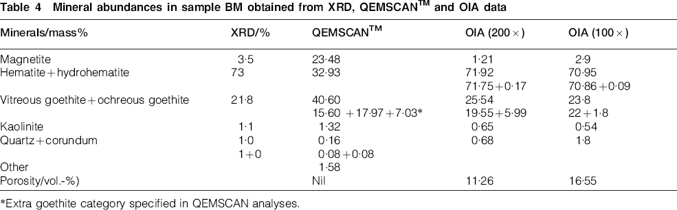
Extra goethite category specified in QEMSCAN analyses.

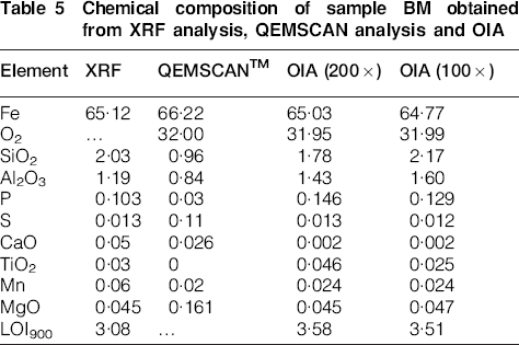
The data on chemical composition obtained by XRF, SEM and OIA for sample BM (Table 5) show that iron and silica are much closer to the XRF results for OIA than for SEM. As for sample RM, SEM identified the lowest amount of hematite plus magnetite, and simultaneously detected the highest total iron content. Alumina was overestimated by OIA relative to XRF analysis, whereas alumina was underestimated by SEM.

Table 5

Chemical composition of sample BM obtained from XRF analysis, QEMSCAN analysis and OIA

Element	XRF	QEMSCAN^TM	OIA (200×)	OIA (100×)
Fe	65·12	66·22	65·03	64·77
O₂	…	32·00	31·95	31·99
SiO₂	2·03	0·96	1·78	2·17
Al₂O₃	1·19	0·84	1·43	1·60
P	0·103	0·03	0·146	0·129
S	0·013	0·11	0·013	0·012
CaO	0·05	0·026	0·002	0·002
TiO₂	0·03	0	0·046	0·025
Mn	0·06	0·02	0·024	0·024
MgO	0·045	0·161	0·045	0·047
LOI₉₀₀	3·08	…	3·58	3·51

Conclusions

Significant progress has recently been made in optical image analysis and SEM characterisation of iron ores. The major iron ore minerals, including magnetite, hematite, vitreous and ochreous goethite, can be identified using both optical and SEM-based techniques. However, both methods have their advantages and disadvantages.

The results for characterisation of two Australian iron ore samples by QEMSCAN and OIA are presented in this paper and show that OIA has significant advantages in identification of microporosity within particles that is critical for textural characterisation and accurate prediction of downstream processing performance. The relatively low resolution during routine QEMSCAN analysis significantly restricts capabilities for comprehensive textural characterisation of iron ores.

Misidentification of minerals by SEM can occur in microporous structures, e.g. microporous hematite or vitreous goethite can be identified as ochreous goethite. Significant misidentification of hematite as magnetite, and vitreous goethite as hematite also occurred for sample BM, although the issues responsible for that need further detailed study to be resolved. During SEM imaging of iron oxides, strong particle edge effects can also be present, resulting in areas of misidentification. This can significantly bias the final information, especially for small particles. Unfortunately software correction for this phenomenon, which is available within the QEMSCAN software and can partially correct boundary areas, was not used for this work.

Scanning electron microscopy cannot currently distinguish hydrohematite from hematite. In contrast, OIA can reliably make this distinction, and in addition can identify different grain and crystal structures, with potential for more development in this area. Automated OIA routines using the CSIRO Recognition3/Mineral3 software can provide high resolution data, with competitive image acquisition and processing times.

Scanning electron microscopy can chemically distinguish a much larger variety of gangue minerals and has advantages in the automated identification of non-opaque gangue minerals, such as quartz. Even though a novel technique for identification of non-opaque minerals by OIA has been developed, it still needs further verification and refinement.

The main conclusion of this study is that, for low iron content ores or tailings, SEM can provide much more detailed information on the gangue minerals than OIA. However, for routine characterisation of iron ores with high iron content and containing a variety of texturally complex iron oxides and oxyhydroxides, OIA is a more cost effective, faster and more reliable method of iron ore characterisation. A combined approach using both techniques provides the most detailed understanding of iron ores.

Footnotes

Acknowledgements

The authors would like to acknowledge CSIRO Process Science and Engineering for funding this work and wish to thank Tirsha Raynlyn and Abebe Haileslassie for sample preparation. Thanks also go to the reviewers of this paper, in particular Ralph Holmes for valuable discussions and editing of this paper.

References

AxioVision, 2006–2009. V 4·8·0·0, Carl Zeiss Imaging Solutions GmbH.

Beukes

, Mukhopadhyay

and Gutzmer

. 2008. Genesis of high-grade iron ores of the Archean Iron Ore Group around Noamundi, India, Econ. Geol., 103, 365–386.

Bonifazi

. 1995. Digital multispectral techniques and automated image-analysis procedures for industrial ore modelling, Miner. Eng., 8, (7), 779–794.

Clout

JMF

. 2003. Upgrading processes in BIF-derived iron ore deposits: implications for ore genesis and downstream mineral processing, Appl. Earth Sci., 112, (1), 89–95.

Clout

JMF

and Simonson

. 2005. Precambrian iron formations and iron formation- hosted iron ore deposits, Econ. Geol., 100th Anniv. Vol., 643–679.

Danti

, Cross

and Halsall

. 1993. A high performance, low cost image analysis system for IBM compatible computers: practical applications in mineral processing and geology, in Programme and Abstracts, International Congress on Applied Mineralogy ‘93, Mineralogy in the Service of Mankind, Fremantle, WA, Australia, May–June, AusIMM, 47–49.

Donskoi

, and Clout

JMF

. 2005. automated textural classification of iron ores using ‘Recognition’ – A specialised software package for studying iron ores. Proceedings, Iron Ore 2005, Fremantle, WA, Australia, September, AusIMM, 203–211.

Donskoi

, Holmes

, Manuel JR , Campbell

, Poliakov

, Suthers

and Raynlyn

. 2008a. Utilization of iron ore texture information for prediction of downstream process performance, Proceedings, 9th International Congress for Applied Mineralogy, Brisbane, Australia, September, 687–693, AusIMM—Australian Institute of Mining and Metallurgy.

Donskoi

, Manuel JR , Clout

JMF

and Zhang

. 2007. Mathematical modeling and optimization of iron ore sinter properties, Israel J. Chem., 47, 373–379.

10.

Donskoi

, Poliakov

, Manuel

, Peterson

and Hapugoda

. 2013. Industrial Strength Optical Image Analysis System – Mineral4/Recognition4, Iron Ore 2013, Perth, WA, Australia, August, AusIMM, 227–241.

11.

Donskoi

, Poliakov

, Manuel JR and Raynlyn

. 2010. Advances in optical image analysis and textural classification of iron ore fines, Proceedings, XXV International Mineral Processing Congress – IMPC2010, Brisbane, Australia, September, 45, AusIMM—Australian Institute of Mining and Metallurgy.

12.

Donskoi

, Poliakov

, Manuel JR and Raynlyn

. 2008b. Development of optical image analysis techniques for improved mineral and texture identification of iron ores, Proceedings, Automated Mineralogy 2008, Brisbane, Australia, September.

13.

Donskoi

, Suthers

, Campbell

and Raynlyn

. 2008c. Modelling and optimization of hydrocyclone for iron ore fines beneficiation – using optical image analysis and iron ore texture classification, Int. J. Miner. Process., 87, 106–119, AusIMM—Australian Institute of Mining and Metallurgy.

14.

Donskoi

, Suthers

, Campbell

, Raynlyn

and Clout

JMF

. 2006. Prediction of hydrocyclone performance in iron ore beneficiation using texture classification. Proceedings, XXIII International Mineral Processing Congress, Istanbul, Turkey, September 2006, 1897–1902, AusIMM—Australian Institute of Mining and Metallurgy.

15.

Figueroa

, Möller

, Buhot

, Gloy

and Haberlah

. 2011. Proceedings, 10th International Congress for Applied Mineralogy (ICAM), Trondheim, Norway, August, 197–204, Springer.

16.

Gomes

ODM

, Paciornik

and Iglesias

JCA

. 2010. A simple methodology for identifying hematite grains under polarized reflected light microscopy, in Proceedings of 17th International Conference on Systems, Signals and Image Processing – IWSSIP, 428–431, Rio de Janeiro, EdUFF.

17.

Gottlieb

, Wilkie

, Sutherland

, Ho-Tun

, Suthers

, Perera

, Jenkins

, Spencer

, Butcher

and Rayner

. 2000. Using quantitative electron microscopy for process mineralogy applications, J. Min., 24–25.

18.

Iglesias

JCA

, Gomes

ODM

and Paciornik

. 2011. Automatic recognition of hematite grains under polarized reflected light microscopy through image analysis, Miner. Eng., 24, (12), 1264–1270.

19.

König

. 2013. Application of X-ray diffraction to iron ores- potential implications for grade control and downstream processing, Proceedings, Iron Ore 2013, Perth, WA, Australia, August, AusIMM, 275–280.

20.

Lane

, Martin

and Pirard

. 2008. Techniques and applications for predictive metallurgy and ore characterization using optical image analysis, Miner. Eng., 21, 568–577.

21.

Maddren

, Ly

, Suthers

, Butcher

, Trudu

and Botha

PWSK

. 2007. A new approach to ore characterisation using automated quantitative mineral analysis. Proceedings, Iron Ore 2007, Perth, Australia, August, AusIMM, 131.

22.

Morris

. 1980. A textural and mineralogical study of the relationship of iron ore to banded iron-formation in the Hamersley Iron Province of Western Australia, Econ. Geol., 75, 184–209.

23.

Pirard

, Lebichot

and Krier

. 2007. Particle texture analysis using polarized light imaging and grey level intercepts, Int. J. Miner. Process., 84, 299–309.

24.

Poliakov

and Donskoi

. 2014. Automated relief-based discrimination of non-opaque minerals in optical image analysis, Miner. Eng., 55, 111–124.

25.

Slayter

EMicroscope

. 1998. Grolier Multimedia Encyclopedia Online. Grolier.

26.

Spencer

. 1919. Mineralogical characters of Turite ( = turgite) and some other iron-ores from Nova Scotia, Mineralog. Mag., 18, 339–348.

27.

Zhang

and Subasinghe

. 2013. Prediction of mineral liberation characteristics of comminuted particles of high grade ores, Miner. Eng., 49, 68–76.