Using production data to improve grade estimation in underground mining

Abstract

All available data should be used to build a geostatistical model. In underground mining, data have different support volumes: drillhole data are defined at a quasi-point support, while production data represent tonnes of ore mined during a period of time (stopes). Due to the support difference, production data are frequently ignored to update the block grade model. We propose a block kriging approach to combine these two sources of information (point and volumetric support data). A synthetic underground mining case is presented. Two estimation scenarios are evaluated: the first considers only drillhole data, while the second considers both drillhole and production data. Results show that the use of production data improves grade estimation. The improvement is more pronounced where diamond drillholes are sparsely located.

Keywords

Block kriging Production data Data support

Introduction

In underground mining, data are available at different support volumes: diamond drillholes are defined at a quasi-point support while production data (grades from stopes mined during a period of time) represent thousands of tonnes. Both data are valuable and should be used in estimation processes. However, the support difference must be considered.

The block kriging approach (Journel and Huijbregts 1978, Isaaks and Srivastava 1989, Goovaerts 1997, Deutsch and Journel 1998) to combine data of different supports is well established in the literature (Deutsch et al. 1996, Yao and Journel 2000, Tran et al. 2001, Kyriakidis 2004, Ren et al. 2005, Pardo-Igúzquiza et al. 2006, Hansen and Mosegaard 2008, Liu and Journel 2009, Poggio and Gimona 2013). However, these studies were applied to either remote sensing or to petroleum geostatistics, where the large support samples have two characteristics:

(i)

they cover the entire study area

(ii)

they all have the same size and shape.

These characteristics do not apply to an underground mining case because production data come from mined stopes, which have irregular shapes and cover partially the estimation area.

We aim to investigate the benefits of using production data to forecast future production in an underground mining scenario. Two cases are investigated: the first (case 1) considers only drillhole samples, while the second (case 2) considers drillhole samples and production data. In each case, the estimates are compared with a reference block grade model.

Methodology

Kriging with coarse-scale data

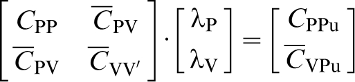
A full description of kriging equations can be found in Goovaerts (1997). We emphasise the incorporation of coarse-scale data into the kriging system. The coarse-scale data (Z_V) are defined as the linear averages of the point values Z(u’) within the volume V (Journel and Huijbregts 1978, Goovaerts 1997, Deutsch and Journel 1998). With coarse-scale data, simple kriging weights are obtained using equation (1) (1) where C_PP denotes point-to-point covariance, denotes point-to-block covariance and denotes block-to-block covariance. Pu designates the point to be estimated, and λ_P and λ_V represent the kriging weights for point and volume average data, respectively. 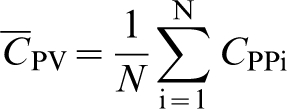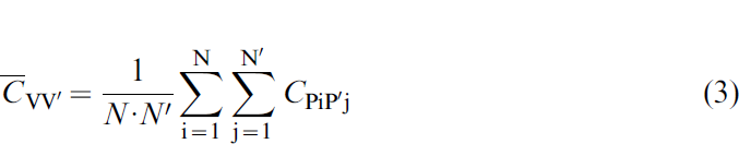C_PPu denotes point-to-point covariance between the data at point support and the point to be estimated and denotes point-to-block covariance between the volumetric average data and the point to be estimated. Point-to-block (equation (2)) and block-to-block (equation (3)) covariance are obtained by averaging point covariances (2) (3) where Pi is the ith of the N points discretising the volume V and P’j is the jth of the N’ points discretising the volume V’.

Case study

The Walker Lake dataset (Isaaks and Srivastava 1989) was modified to resemble an underground deposit, and the variable V was used. Firstly, the coordinates were modified: the original Y (north) became Z coordinates (elevation). Then, the high-grade regions and the stope cross sections were delimited using computer-aided design software. The limits were expanded in the north direction to become three-dimensional solids. A block model whose block size was 5×5×5 m was created. The blocks inside the orebody solids were flagged as ore and represent our geostatistical domain (Fig. 1). The grey blocks in Fig. 1 represent the stope cross sections. We assume that this synthetic scenario characterises a gold mine, so the variable V expresses gold grade (g t⁻¹) and the production is measured in grams.

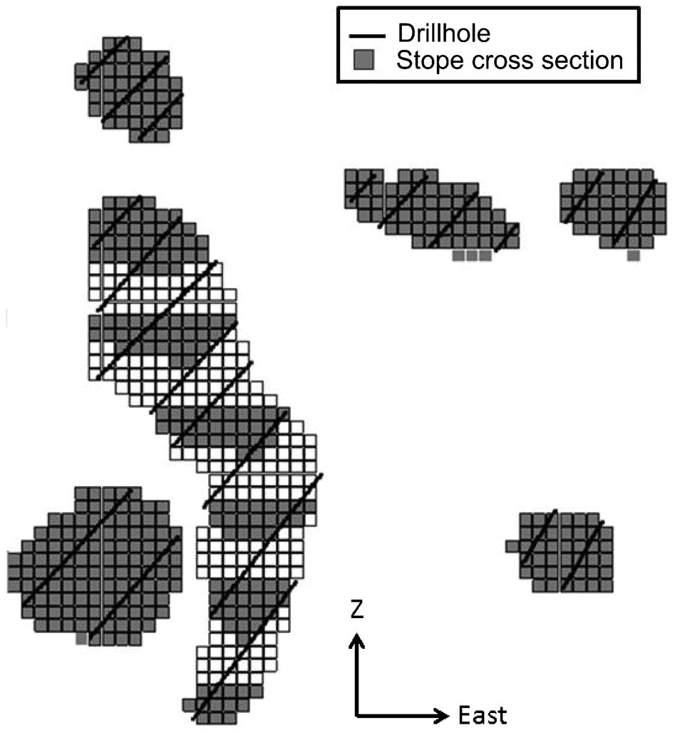
Block model, stope cross sections and drillholes

Reference block grade model

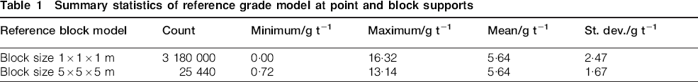
First, we selected the V samples of the Exhaustive Walker Lake Dataset (Isaaks and Srivastava 1989) inside the orebody solids. These points provided a probability density function to condition the sequential Gaussian simulation. Second, we discretised the ore blocks (size 5×5×5 m) into blocks of size 1×1×1 m and ran a sequential Gaussian simulation in this dense grid. This model is our reference grade model at the point support (Fig. 2a). Finally, the simulated points were block averaged to the original block size of 5×5×5 m to obtain the reference grade model at the block support (Fig. 2b). The reference block grade model contains the true grade of each block. Table 1 shows summary statistics of the reference grade models at point and block supports. Both models have the same mean, but the variance is higher for the point-support case.

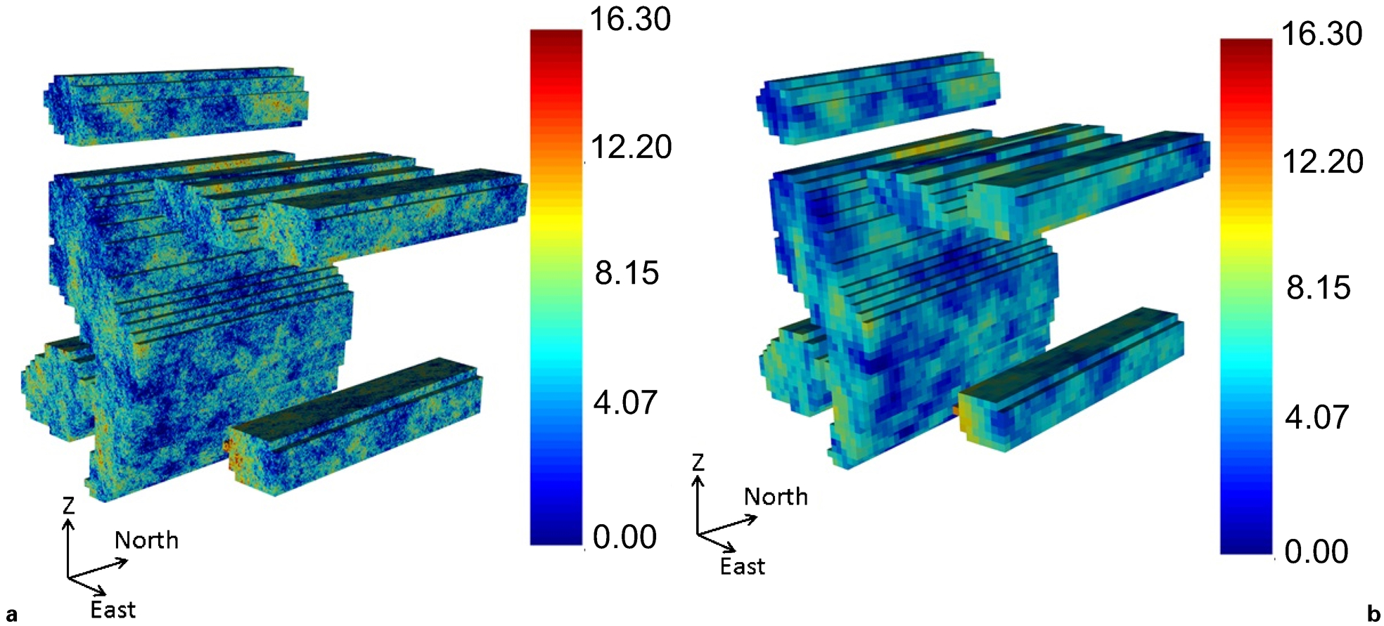
a reference point-support grade model; b reference block-support grade model

Table 1

Summary statistics of reference grade model at point and block supports

Reference block model	Count	Minimum/g t⁻¹	Maximum/g t⁻¹	Mean/g t⁻¹	St. dev./g t⁻¹
Block size 1×1×1 m	3 180 000	0·00	16·32	5·64	2·47
Block size 5×5×5 m	25 440	0·72	13·14	5·64	1·67

Dataset presentation

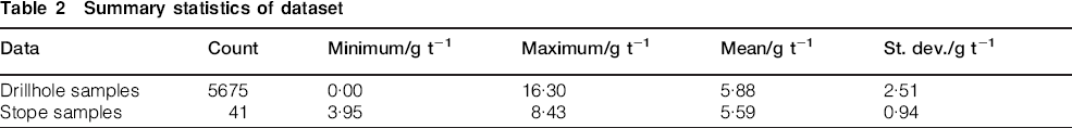
The samples were collected at two distinct supports. The drillhole samples are at quasi-point supports. In contrast, the stope samples represent ore blocks that have been previously mined. A group of blocks forms a stope. Dilution and ore losses are ignored. Basic statistics for these data are shown in Table 2.

Table 2

Summary statistics of dataset

Data	Count	Minimum/g t⁻¹	Maximum/g t⁻¹	Mean/g t⁻¹	St. dev./g t⁻¹
Drillhole samples	5675	0·00	16·30	5·88	2·51
Stope samples	41	3·95	8·43	5·59	0·94

Drillhole samples

The drillholes align along east–west and dip roughly by 45° (see black lines in Fig. 1). The drillhole samples are 1 m long and are retrieved from the dense reference model (block size of 1×1×1 m). At higher elevations (Z), the orebody is densely sampled with drillholes (Fig. 3). However, at lower levels, the orebody is poorly sampled with drillholes (Fig. 3). This situation occurs when drilling operation fails to follow accordingly the development and production pace.

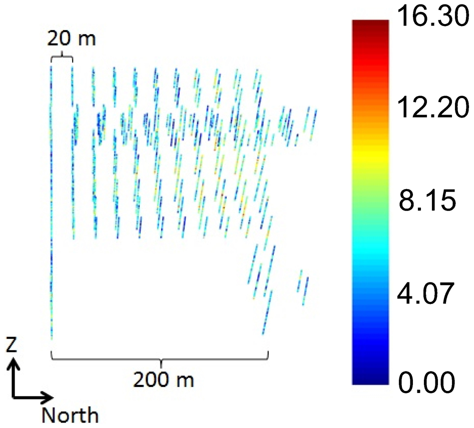
Location map for drillhole samples. At higher levels, orebody is densely sampled with drillholes. At lower levels, orebody is poorly sampled with drillholes

Stope samples

The stope cross-sections (see grey blocks in Fig. 1) were extruded 200 m along the strike direction to make a three-dimensional solid. Then, the resulting solid was divided into solids of 30 m along the north direction. The ore blocks inside each of these solids represent one stope. The scenario considers two types of stopes:

(i)

mined stopes (light grey blocks in Fig. 4a), whose grades are known and represent the stope samples

(ii)

stopes to be mined (dark grey blocks in Fig. 4a), whose grades are unknown and will be estimated.

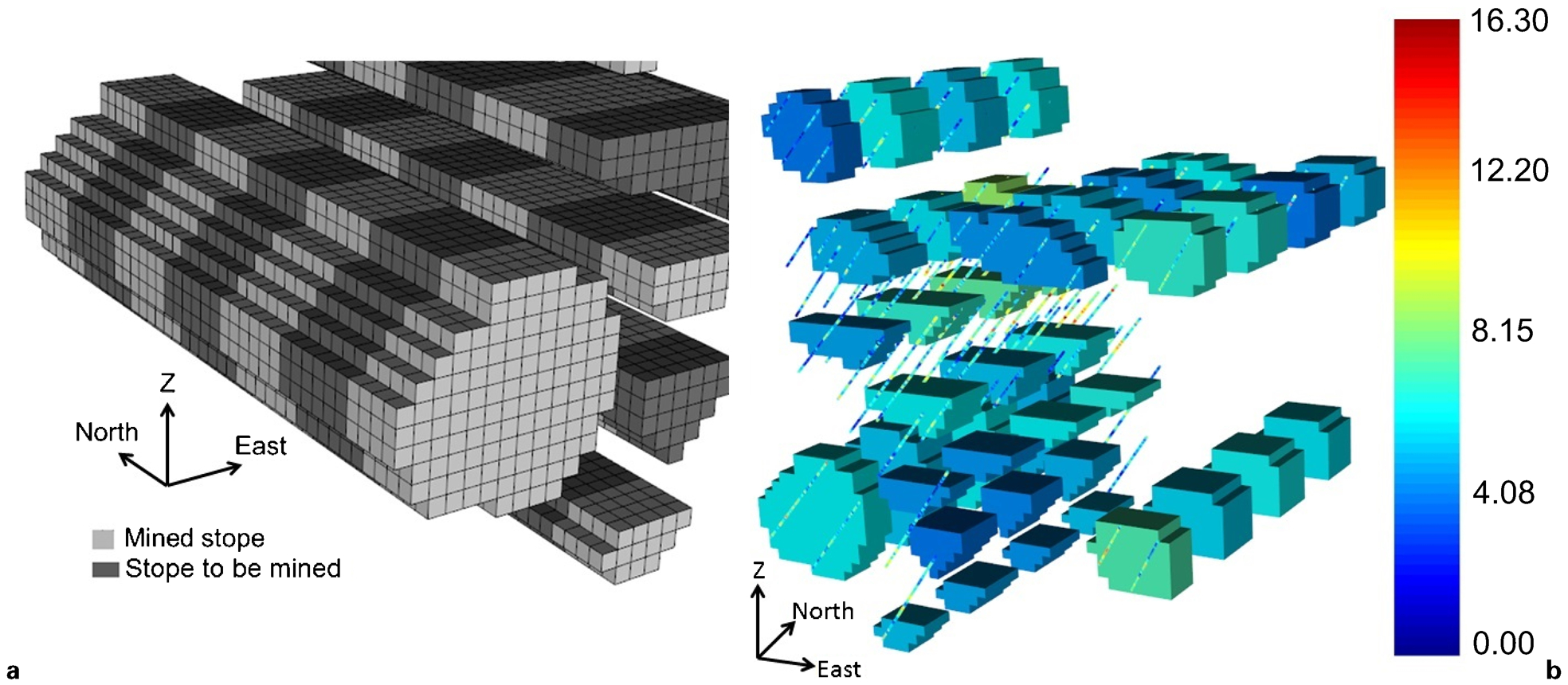
a mined stopes and stopes to be mined; b dataset with drillhole and stope samples

Along the north direction, a mined stope is followed by a stope to be mined (see Fig. 4a). This situation resembles underground mining with sublevel stopping and recovery of secondary stopes (Hartman 1992). The mined-out stopes represent the primary stopes, which were mined and backfilled, and the stopes to be mined represent the secondary stopes to be recovered. The stope grade is the average grade of the blocks (taken from the reference grade model) inside the stope geometry. The full dataset consists of both the drillhole and the stope samples (Fig. 4b).

Estimation

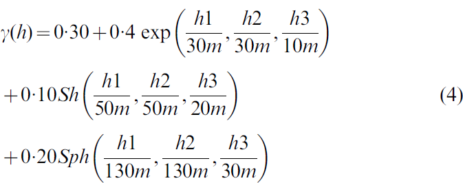
The estimation was carried out using ordinary kriging. Two cases were evaluated: case 1 considers only drillhole samples and case 2 considers both drillhole and stope samples. The variogram model used in the estimates is defined in equation (4) (4) where h1 is the distance along the direction of major continuity (N90°E/−67·5°), h2 is the distance along the direction of intermediate continuity (N0°/0°) and h3 is the distance along the direction of minor continuity (N90°W/−22·5°).

As the software developed performs estimation at point support, the blocks of 5×5×5 m were discretised into eight points regularly spaced at 2·5×2·5×2·5 m. The block estimate is the linear average of its eight discretising points. Tests proved that a finer discretisation increased the processing time and did not affect the final block estimates. Then, the block estimates were averaged according to the stope geometry to obtain the final stope estimate.

Comparison with true grade

Although the average grade of the estimated blocks inside the stope sample geometry equals the stope sample grade for case 2 (block kriging approach), this is irrelevant because they were already mined. We are interested in improving the future production forecast. As future production comes from the stopes to be mined, the results section compares specifically their estimates with their true grade (obtained through the reference grade model). The total number of stopes to be mined is 36. Specifically, 20 stopes are in the densely sampled area, while 16 stopes are in the poorly sampled area.

The stope estimates were compared with their true grade (obtained from the reference block model) using scatterplots. Moreover, the estimation errors were evaluated for each stope. The comparisons were carried out first considering all stopes to be mined. Then, the comparisons were repeated for densely and poorly sampled areas separately.

Impact on production forecast

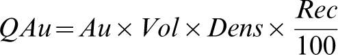
For each stope, the predicted metal quantity was compared with the true metal quantity produced. Equation (5) defines the metal quantity (QAu) in grams (5) where Au denotes the gold grade (g t⁻¹), Vol denotes the stope volume (m³), Dens denotes the stope density (t m⁻³) and Rec denotes the metallurgical recovery (%). Metallurgical recovery (Rec) and density were considered constant at 90% and 2·60 t m⁻³ respectively. The difference between the estimated and true metal quantity produced was measured.

Results and discussion

Scatterplots

Figure 5 shows the scatterplot between the true and estimated stope grades for case 1 (Fig. 5a) and case 2 (Fig. 5b). The stope grades located in the highly sampled area (black dots in Fig. 5a and b) are roughly equally scattered for case 1 (Fig. 5a) and for case 2 (Fig. 5b). The stope grades located in the poorly sampled area (red dots in Fig. 5a and b) are less scattered for case 2 (Fig. 5b) than for case 1 (Fig. 5a).

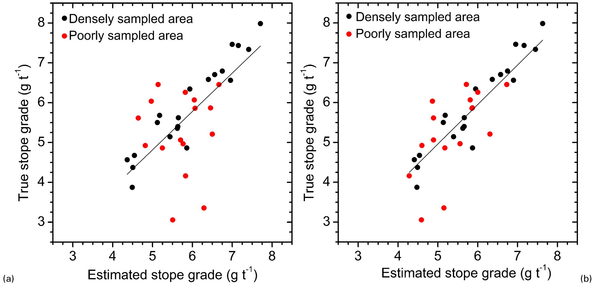
Scatterplot of true and estimated stope grades: a case 1; b case 2

Table 3 presents the slope of the linear regression (y = ax) and the correlation coefficient between the estimated and true stope grades. Considering the total number of stopes, the slope of the linear regression and the correlation coefficient are closer to 1 for case 2. The improvement is due to the additional information provided by the stope samples.

Table 3

Slope of linear regression and coefficient of correlation between true and estimated stope grades

Stopes considered	Count	Slope		Correlation
Stopes considered	Count	Case 1 (drillholes)	Case 2 (drillholes+stopes)	Case 1 (drillholes)	Case 2 (drillholes+stopes)
Total	36	0·96	0·99	0·73	0·85
Densely sampled area	20	1·00	1·00	0·95	0·95
Poorly sampled area	16	0·91	0·97	0·07	0·54

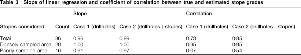
In the densely sampled area, case 1 and case 2 showed similar slopes of the linear regression and correlation coefficients with the reference grade model (Table 3). Kriging weights are higher for samples that are more spatially correlated to the points to be estimated. This spatial correlation is lower for the samples that are distant from the points to be estimated. In the densely sampled area, the stope samples are more distant from the points to be estimated than the drillhole samples and received low kriging weights (along the north–south direction, the drillholes are 20 m apart, while the stope centroids are 60 m apart). Consequently, the stope samples only slightly affected the estimates in the densely sampled area.

In the poorly sampled area, case 2 showed the slope of regression and correlation coefficient much closer to 1 than case 1 (Table 3). The low coefficient of correlation for both cases is partially due to the small number of stopes. In this region, the stope samples are more correlated to the points to be estimated than the drillhole samples and have higher kriging weights. As the stope samples are more correlated with the points to be estimated than the drillhole samples, the use of stope samples improved the estimates.

Estimation error

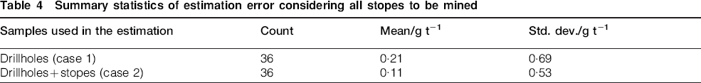
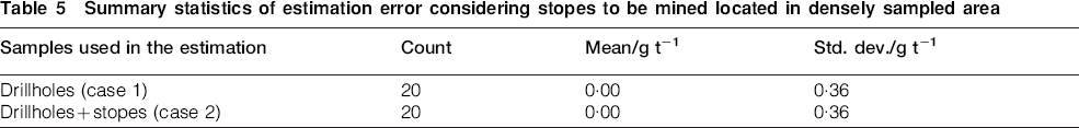
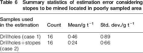
Considering all the stopes to be mined (Table 4), the mean and standard deviation of the estimation error were lower in case 2 than in case 1. In the densely sampled area (Table 5), the mean and standard deviation of the estimation error were low for the two cases. In the poorly sampled area, the mean and standard deviation of the error were significantly lower in case 2 than in case 1 (Table 6). As mentioned, the stope samples improved the estimates when they were more correlated to the points to be estimated than the other samples (poorly sampled area). The addition of the stope samples resulted in estimates that were more accurate (mean error closer to zero) and more precise (lower standard deviation of the error).

Table 4

Summary statistics of estimation error considering all stopes to be mined

Samples used in the estimation	Count	Mean/g t⁻¹	Std. dev./g t⁻¹
Drillholes (case 1)	36	0·21	0·69
Drillholes+stopes (case 2)	36	0·11	0·53

Table 5

Summary statistics of estimation error considering stopes to be mined located in densely sampled area

Samples used in the estimation	Count	Mean/g t⁻¹	Std. dev./g t⁻¹
Drillholes (case 1)	20	0·00	0·36
Drillholes+stopes (case 2)	20	0·00	0·36

Table 6

Summary statistics of estimation error considering stopes to be mined located in poorly sampled area

Samples used in the estimation	Count	Mean/g t⁻¹	Std. dev./g t⁻¹
Drillholes (case 1)	16	0·46	0·89
Drillholes+stopes (case 2)	16	0·24	0·66

Production forecast

Figure 6 shows the absolute difference between the true and forecasted metal quantity for each stope. In the densely sampled area (stope index 1–20 in Fig. 6), the two cases have similar distances from the zero line. However, in the poorly sampled area (stope index 21–36 in Fig. 6), case 2 is closer to the zero line than case 1. An exception occurred at the stope whose index is 31.

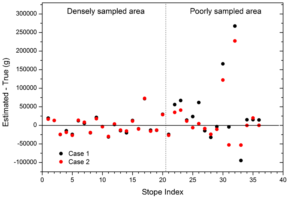
Absolute difference between estimated and true metal quantity for each stope. Stope index 1–20 refers to stopes located in densely sampled area while stope index 21–36 refers to stopes in poorly sampled area

Considering the total amount of grams estimated in the two cases, case 2 is closer to the true amount of grams obtained (Table 7). In case 1, the grade model overestimates roughly 3·70% of the metal quantity, while in case 2, this difference drops to 1·94%.

Table 7

Estimated and true grams produced

Estimated – case 1/g	Estimated – case 2/g	True/g
14 711 815·10	14 460 837·95	14 185 528·89

We found that the use of production data improved the prediction of metal content in an underground mining scenario. The greatest improvements occurred when the production data were more correlated with the points to be estimated than the other samples. Overall, the use of volumetric data reduced the mean and standard deviation of the estimation error, showed a better slope of the linear regression and coefficient of correlation with the true grades, and predicted better the in situ metal content.

Direct use of stope grades for updating the short term grade model in some mining situations would demand other alternatives than the one presented. It is known the stope grades may be strongly affected by dilutions or losses. If the stope samples are biased and imprecise, one could consider using the block cokriging methodology (Deutsch et al. 1996). Similarly to the block kriging presented, block cokriging can cope with data of different support through average covariances.

The use of production data for estimation is not a novelty. What is herein introduced is how data in different support (volumetric in this example) can be incorporated in the kriging system. Commercial softwares available do not allow practitioners to combine data of different volume because the algorithms cannot average covariances between data of different volumes. The synthetic case study was selected to demonstrate the functionality of the methodology that can be extended to other mining scenarios. For instance, grades at volumes mined monthly in an open pit mine can be used to update grade models similarly. The challenge to incorporate large volume samples (i.e. stopes) effectively for estimation is to know their spatial location, shape, and mean grade reasonably well.

Conclusion

In summary, the study showed that the use of production data improved grade estimation in a synthetic underground mining scenario. The benefits were evident when the production data were more correlated to the points to be estimated than the drillholes. Although, in the mining industry, production data are often ignored for estimation, this study showed that they can provide valuable information. Moreover, the study demonstrates the usefulness of the block kriging methodology to incorporate data of distinct support.

Footnotes

Acknowledgements

The authors would like to thank Capes, CNPq (research agencies in Brazil), PETROBRAS S.A, and VALE S.A. for the financial support.

References

Deutsch

, Srinivasan

and Mo

. 1996. Geostatistical reservoir modeling accounting for precision and scale of seismic data. SPE Annual Tech. Conf., Denver, CO, USA, 6–9 October 1996.

Deutsch

and Journel

. 1998. GSLIB: Geostatistical software library and user's guide. New York: Oxford University Press.

Goovaerts

. 1997. Geostatistics for natural resource evaluation. Oxford: Oxford University Press.

Hansen

and Mosegaard

. 2008. Visim: sequential simulation for linear inverse problems. Computers & Geosciences, 34 (1), pp. 53–76.

Hartman

HLed

. 1992. SME mining engineering handbook. Littleton, CO: Soc. for Mining, Metallurgy, and Exploration, Inc.

Isaaks

and Srivastava MR . 1989. An introduction to applied geostatistics. Oxford: Oxford University Press.

Journel

and Huijbregts

. 1978. Mining geostatistics. New York: Academic Press.

Kyriakidis

. 2004. A geostatistical framework for area-to-point spatial interpolation. Geographical Analysis, 36, pp. 259–89.

Liu

and Journel

. 2009. A package for geostatistical integration of coarse and fine scale data. Computers & Geosciences, 35 (3), pp. 527–47.

10.

Pardo-Igúzquiza

, Chica-Olmo

and Atkinson

. 2006. Downscaling cokriging for image sharpening. Remote Sensing of Environment, 102 (1–2), 86–98.

11.

Poggio

and Gimona

. 2013. Modelling high resolution RS data with the aid of coarse resolution data and ancillary data. International Journal of Applied Earth Observation and Geoinformation, 23, pp. 360–71.

12.

Ren

, McLennan

, Cunha

and Deutsch

. 2005. An exact downscaling methodology in presence of heterogeneity: application to the Athabasca Oilsands. SPE Int. Thermal Operations and Heavy Oil Symp., Calgary, Alberta, Canada, 1–3 November 2005.

13.

Tran

, Deutsch

and Xie

. 2001. Direct geostatistical simulation with multiscale well, seismic, and production data. SPE Annual Tech. Conf. and Exhibition, New Orleans, LA, USA, 30 September–3 October 2001.

14.

Yao

and Journel

. 2000. Integrating seismic attribute maps and well logs for porosity modeling in a west Texas carbonate reservoir: addressing the scale and precision problem. Journal of Petroleum Science and Engineering. 28 (1–2), pp. 65–79.