
Abstract
Choosing a resource estimation approach for uranium deposits central Jordan needs to consider various issues; the particular geological context of these deposits, the varying degree of reliability of input data and the level of selectivity that can be reasonably envisaged at a production stage. These issues make this resource estimation challenging from a geostatistical perspective. Here, we provide details of the approach used during resource estimation for the surficial part of uranium deposits in central Jordan; as a more standard approach has been applied to the deeper parts of these deposits. The workflow is as follows:
Interpolation of the geometry of the mineralised formation. Kriging with external drift is applied to model hangingwall and footwall surfaces. Estimation of global resources by 2D estimation of layer thicknesses and uranium accumulation using channel samples within delineated areas. Accounting for vertical selectivity and development of grade tonnage curves using uniform conditioning (UC) followed by localised post-processing (called LUC) delivering, a 3D block model at the selective mining unit support scale.
A description of the UC/LUC approach and the adaptations made in order to account for the variable thickness is presented in this paper. This approach involves performing UC on each panel in turn with a thickness varying from panel to panel. This leads to a specific change of support coefficients for each panel. The illustrations of this approach are taken from one specific zone within the Central Jordan deposits.
Introduction
The exploration of the Central Jordan uranium deposits has been conducted in several drilling phases. This generated a large number of samples that were assayed for uranium (U) content by means of inductively coupled plasma-mass spectrometry (ICP-MS) and radiometric measurements have also been collected over several zones covering a large area (∼130 km2).
Two distinct uranium bearing formations have been identified in Central Jordan:
the first formation contains higher U3O8 grades. It is embedded in surficial carbonate layers down to a maximum depth of approximately 5 m; the second formation lies beneath the surficial uranium layers within the carbonate facies of the Muwaqqar Chalk-Marl Formation.
The surficial deposits show the best potential in terms of metal content, and they are immediately accessible. Consequently, an intense program of trenching, sampling, and assaying was undertaken for the purpose of resource delineation and estimation. A significant number of channel samples have been obtained in some of the aforementioned zones. The spacing of channel samples is finer than the spacing for the borehole samples (Fig. 1).
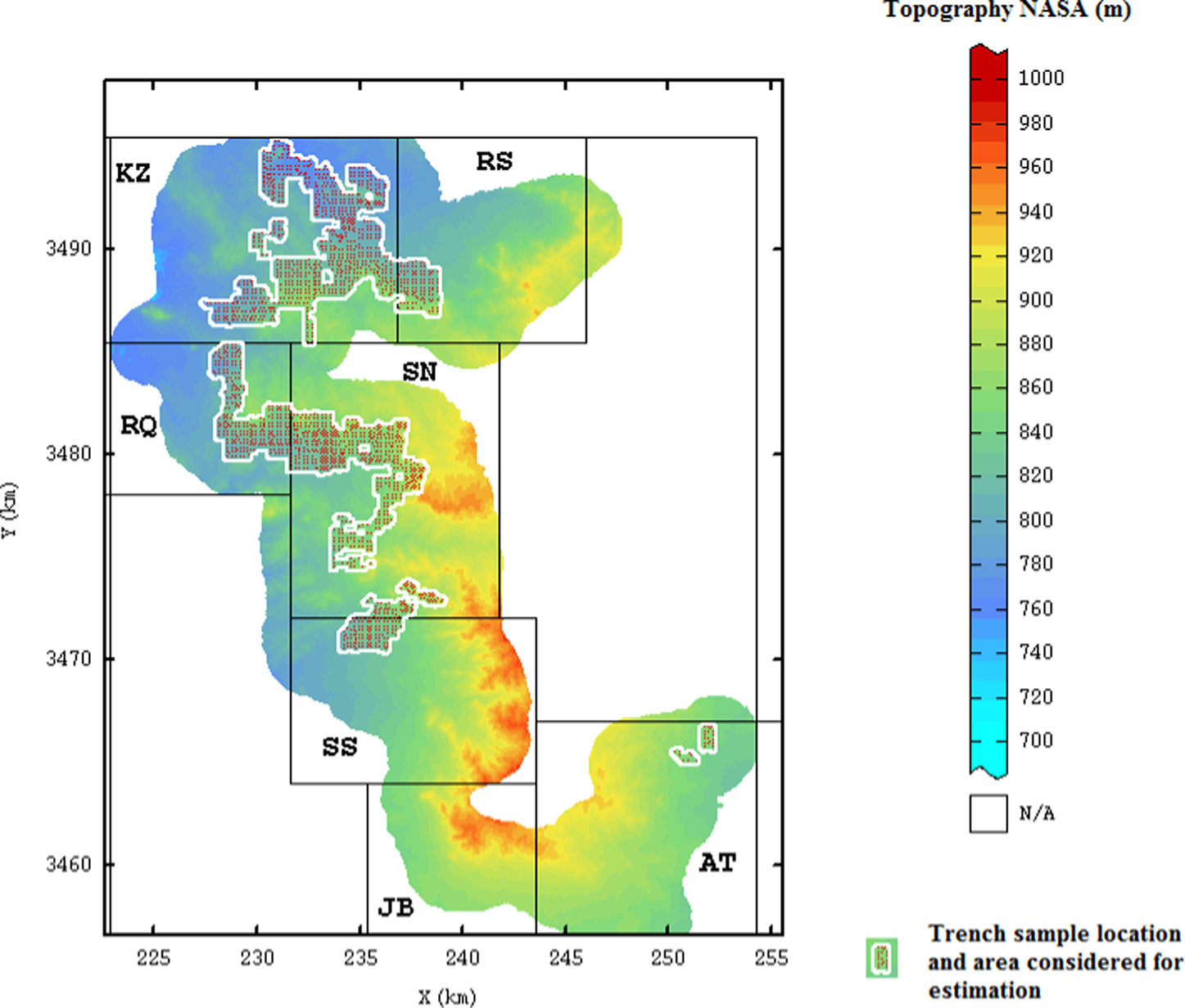
Topographic map of the Central Jordan deposits showing the delineation of zones and the location of sampling trenches
The resource estimation for the first formation highlights specific issues resulting from the low thickness of the formation and the requirements of selective mining.
Two possible approaches have been developed to overcome these issues. These are summarised below:
A 2D approach, which starts with the modelling of the hangingwall and footwall surfaces. The thickness and the accumulation of uranium over this thickness are then co-Kriged. This method is appropriate to estimate in situ resources, i.e. over the whole thickness of the geological formation, but cannot accuarately account for vertical selectivity. The best that can be done is to apply a cutoff grade on the drillhole or channel grade profile to determine the ‘mineable’ hangingwall and footwall. This approach is not satisfactory for the following reasons:
it does not take into account the support effect, in other terms the cutoff has to be applied on a large volume rather than on a drillhole; if the cutoff is changed, the entire estimation has to be redone. As such, this approach is not presented in this paper. A 3D approach was adopted as soon as the selectivity degree was achievable during production. This approach is represented by the geometry of a selective mining unit (SMU). In the present case, a vertical selectivity of 50 cm has been considered. The methodology resorts to non-linear geostatistical models (Rivoirard 1994) and has been successfully applied on channel samples from the study area. A final localisation post-processing step aims to providing a 3D block model with grades at the SMU support level.
General information on the geology of the study area and the data used during this study
For a detailed presentation of the geology, the reader should refer to more specific papers available in this special issue. Here present only the most important aspects that condition the estimation methodology.
Geology
The mineralisation occurs in relation to a surface named ‘MCM’, which is visible in the first 5 m below the topography.
The MCM surface usually coincides with the centre of the mineralised zone. Figure 2 illustrates that the grade profile decreases as soon as the distance to the MCM surface increases.
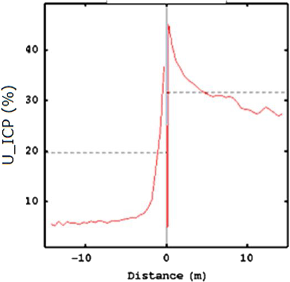
U grade profile as a function of the distance to the MCM surface (negative above, positive below). The dotted lines represent the mean grade of samples above or below the contact surface
This surface is considered as a continuous surface throughout the whole area covered by the deposit. This key role enables the modelling of the MCM surface as accurately as possible and constitutes the first step of the modelling process dealing with the geometry of the surficial mineralisation. Two difficulties should be noted:
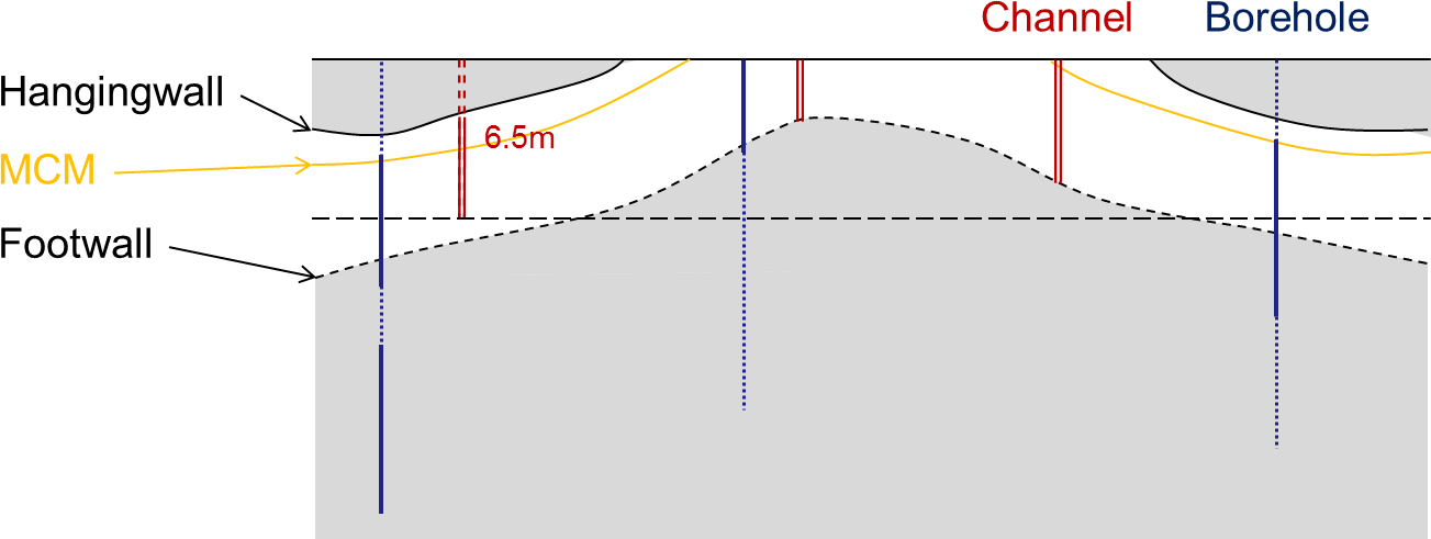
the MCM surface and the hangingwall can be locally eroded. At the modelling stage, the surfaces are interpolated from hard data when the contact is visible and from ‘virtual’ data where the topography has eroded the surficial formation. These virtual data are obtained by generating a value above the topography using Kriging with inequality (Chilès and Delfiner 2012; pp. 558–561). At the end, these surface models are locally eroded to match the topography. In some locations, the footwall surface lies deeper than the maximum trench depth of 6.5 m. It is impossible to extrapolate below the deepest trench level. As a consequence, the estimation models discussed here exclude some potential resources. In the scope of selective mining, it is likely that these resources will not be recovered because of lower grades due to the distance to the MCM surface (Fig. 3). Schematic vertical section of the surficial deposit. The mineralised layer is defined between hangingwall and footwall surfaces. It is sampled by channels that have depths bounded by either the footwall or a technical limit of 6.5 m. Boreholes drilling constrains the elevation of the MCM surface; these boreholes have depths that exceed the channel depth in order to cross instersect any potential uraniferous layers at depth
Data
It should be noted that the elevation of the MCM surface is defined by boreholes only.
The channel data are analysed continuously by intervals of 50 cm from the beginning of the mineralisation, here defined as the hangingwall elevation, to the trench bottom, here defined as the footwall elevation. The U_ICP grade is analysed in laboratories. The radiometric measurements that are impacted by radioactive disequilibrium cannot be easily related to uranium concentrations, meaning that these data were not used during resource estimation; only chemical analyses were used during this estimation.
The area illustrated here contains channel samples at a 200-m mesh, which is centred in some areas (Fig. 4).
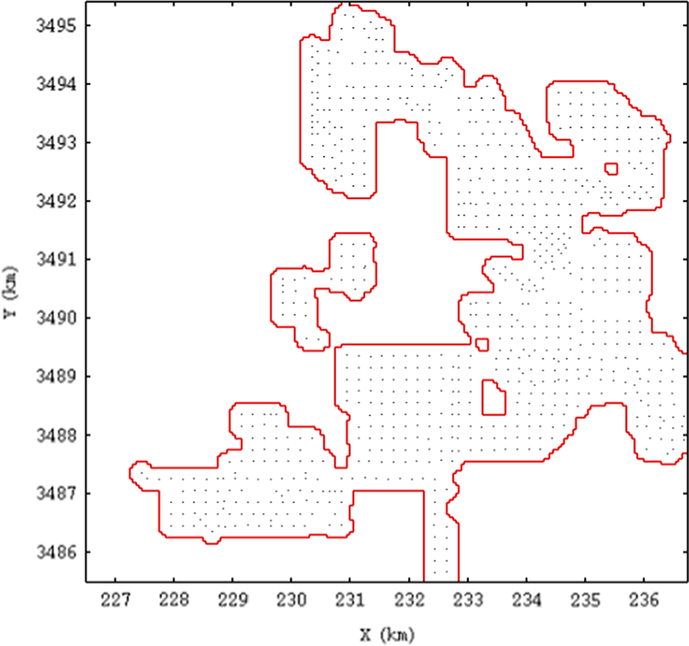
Location map of the channel samples and area considered for resource estimation
The comparison with borehole assays reveals some systematic differences, primarily due to core recovery difficulties. This implies that both data from channels and boreholes cannot be simply merged together. In areas only constrained by trenches, only channel samples have been used. It was assumed that the necessary quality control of these data has been made with state of the art methods.
Methodology
The estimation process involves two different steps:
2D modelling of the surfaces that controls the surficial mineralisation, i.e.:
the topographic surface the MCM surface and the hangingwall and footwall surfaces. 3D modelling of U grades taking into account the mining selectivity between the hangingwall and footwall surfaces. The main steps of the procedure are:
unfolding (flattening) of the composited 50 cm channel data and the SMU grids parallel to the hangingwall surface defined on the 50 × 50 m 2D grid definition of the 3D variogram model from U_ICP data measured in all channels in the unfolded space estimation of panels of 200 × 200 m × variable height modelling the distribution of the SMUs, i.e. applying support correction to the punctual anamorphosis uniform conditioning (UC; Deraisme et al., 2008) of the panels and localisation (LUC) (Abzalov 2006) of SMU grades constrained by the panels grade tonnage curves and back-folding (unflattening) of the SMU grid to the real space.
2D surface modelling
The four surfaces have been modelled from the most reliable available data.
The topography has been interpolated by means of Kriging with external drift (Chilès and Delfiner 2012) from borehole collars, with external drift provided by a NASA topographic model at a fine resolution. The high linear correlation between borehole collars and NASA topography data at those locations (Fig. 5) justifies the use of this method, with this approach yielding a consistent topographic model, controlled by the general shape of the NASA model. The MCM surface was interpolated by Kriging with external drift from boreholes with external drift provided by the previously obtained topographic model. An anisotropic variogram has been fitted on the exact MCM elevation values and was applied during Kriging with inequality including exact and inexact data, with inexact means that the only thing known is that the MCM elevation is above the topography (Figs. 6 and 7). The hangingwall and footwall surfaces were then interpolated from the channel data using MCM as an external drift measurement. This is justified by the linear correlation between the channels and the MCM elevation migrated from the previous model (Fig. 8).
The cross validation of the variogram model based on the channel data was undertaken by: it consists of interpolating the data from the neighbouring data and performing statistical analysis of the numerically computed error. The result is satisfactory and leads to the acceptance of the model (Fig. 9).
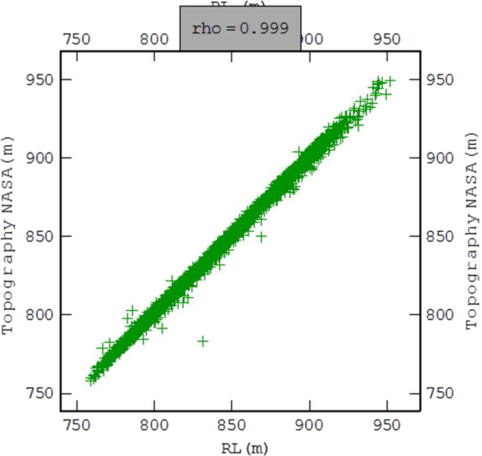
Scatter diagram between Z collars of the boreholes and the NASA topography
Base map of boreholes (dots are for ‘inexact’ data as defined above) and variograms of MCM elevation in four directions from the exact data. Diagram at the bottom shows a histogram of the number of pairs used for each distance
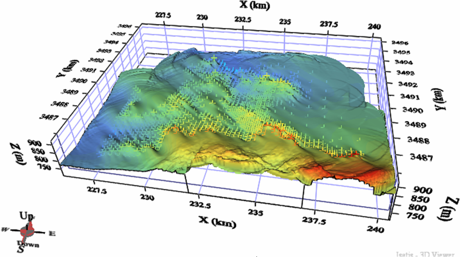
Interpoled MCM surface before topographic erosion
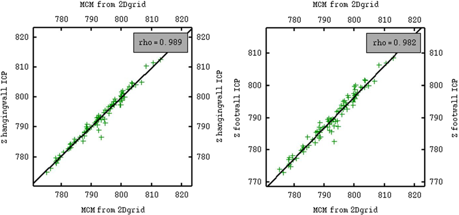
Scatter diagram between hangingwall (left) and footwall (right) elevations of channels and the MCM surface elevation
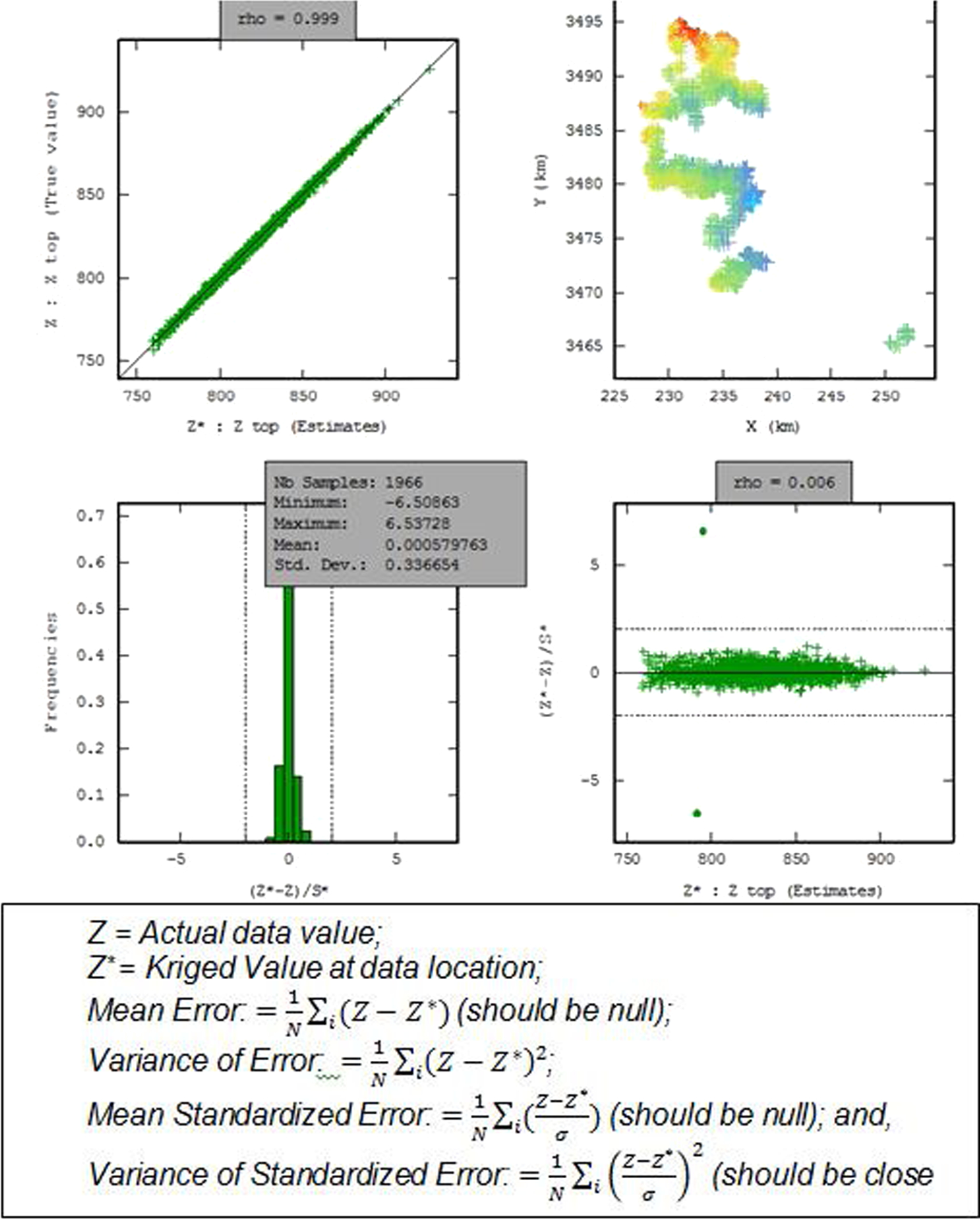
Cross-validation of the hangingwall surface by Kriging with external drift method. Outliers in the lower right graphic are because of two duplicates. Their Kriging standard deviation (here denoted as S*) is close to zero; therefore, the standardised error takes high values (in absolute value)
Modelling of 3D recoverable resources
The estimation of recoverable uranium resources (i.e. after cutoff on a SMU support) by means of non-linear techniques like uniform conditioning (UC) should be adequate and efficient for this study, although the following issues need to be taken into consideration for:
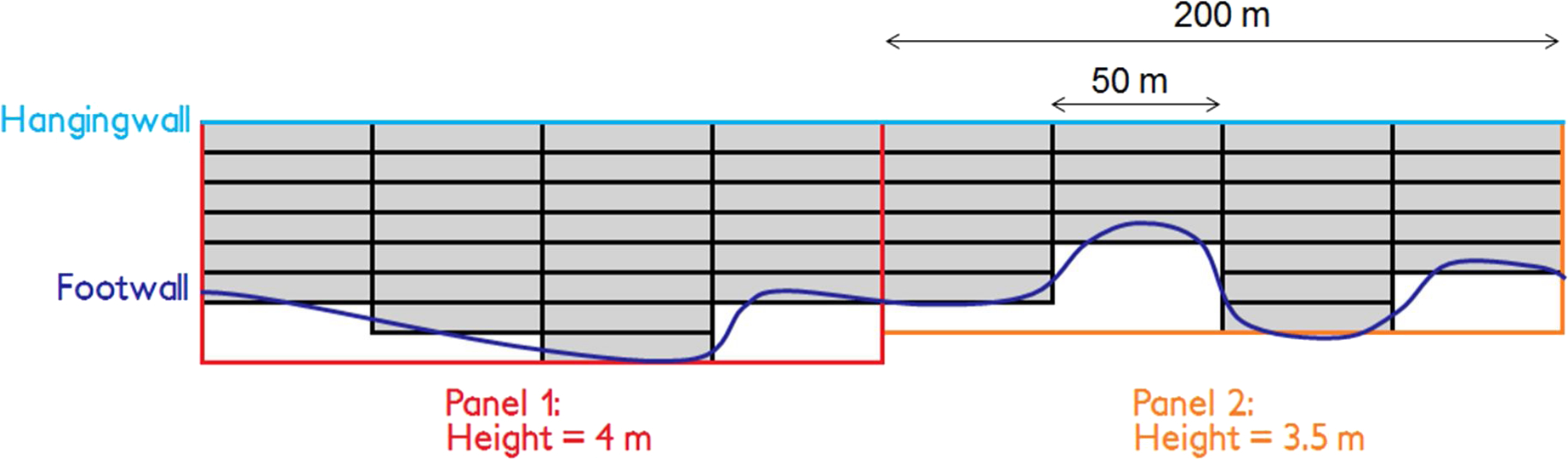
The number of SMUs along the vertical extent of the deposit depends on the variable thickness obtained by determining the difference between the interpolated hangingwall and footwall. This implies that the UC method, based on a fixed partition of panels into SMUs, has to be adapted (Fig. 10). This estimation has to account for the higher level of continuity when following geological marker like the MCM surface. Performing this estimation in a space deformed to follow a reference surface seems like an adapted solution. It has been applied despite a real drawback in that the unfolding used does not preserve the distances. This means that a block of fixed dimension in the real space is not transformed into a block with the same dimensions in the unfolded space, but rather it looks more like a distorted block with its shape varying according to the degree of folding. When dealing with Kriging point estimation is performed on a fine-resolution grid in the flat space, then the Kriged points are transferred to the real space, to be finally averaged in the final blocks. In the present case, this approach is not practicable because it:
model the distribution of the SMU grades, a modelling step that cannot be performed on distorted geometry locally conditions the SMU distribution to Kriged panels informed by two variables: the Kriged estimate and the dispersion variance of those estimates. The latter cannot be simply obtained from point Kriging estimates. Schematic vertical section with the geometry of panels 200 × 200 m and a variable thickness partitioned in different numbers of SMUs 50 m × 50 m × 50 cm in the flattened space
No perfect solution exists to this problem, and the final choice was to perform the estimation in the unfolded space obtained by vertical flattening. The SMU distribution was then derived for a geometry of the SMUs in the flat space that is equivalent to that of the actual SMUs in the original space. This decision is based only the observation that the most important factor for the selectivity is the vertical dimension and that the geometrical distortion of the 50 m × 50 m × 50 cm SMUs during the flattening process is not that important. The whole UC/LUC procedure is then performed in the flat space and the resulting SMU block model transferred back into the real space.
3D estimation of recoverable resources
The histogram of grades composited to 50 cm is modelled after the flattening by means of a Gaussian anamorphosis function (Φ). Raw grades Z(x) are transformed into Gaussian grades Y(x) through the function Z(x) = Φ[Y(x)].
Preliminarily declustering weights were calculated to account for irregular sampling. A cell declustering method was implemented using a 200 × 200 × 0.5 m moving window (Fig. 11).
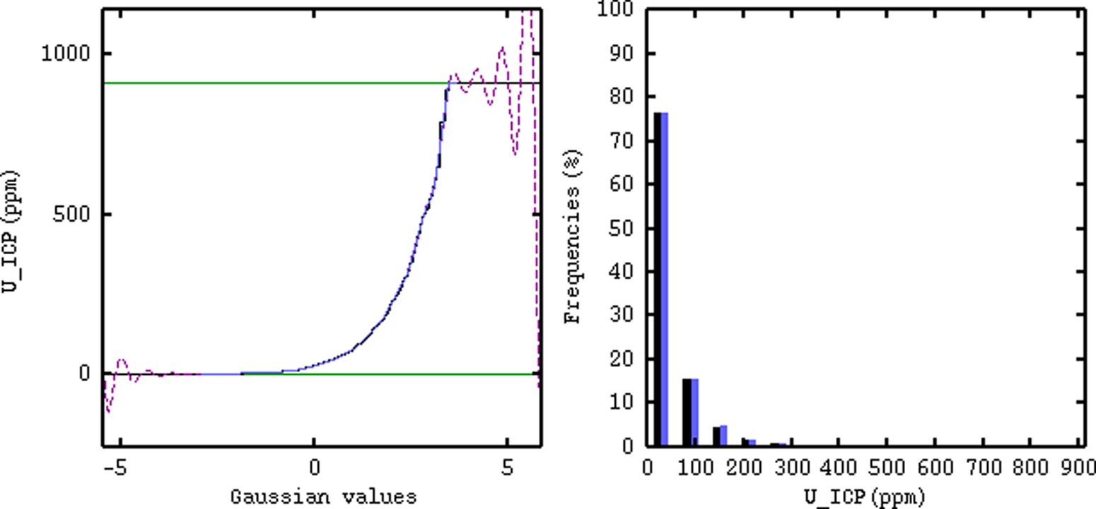
Gaussian anamorphosis function (on left) and histogram on the 50 cm support (on right). Black columns represent experimental data, the blue columns represent modelled data
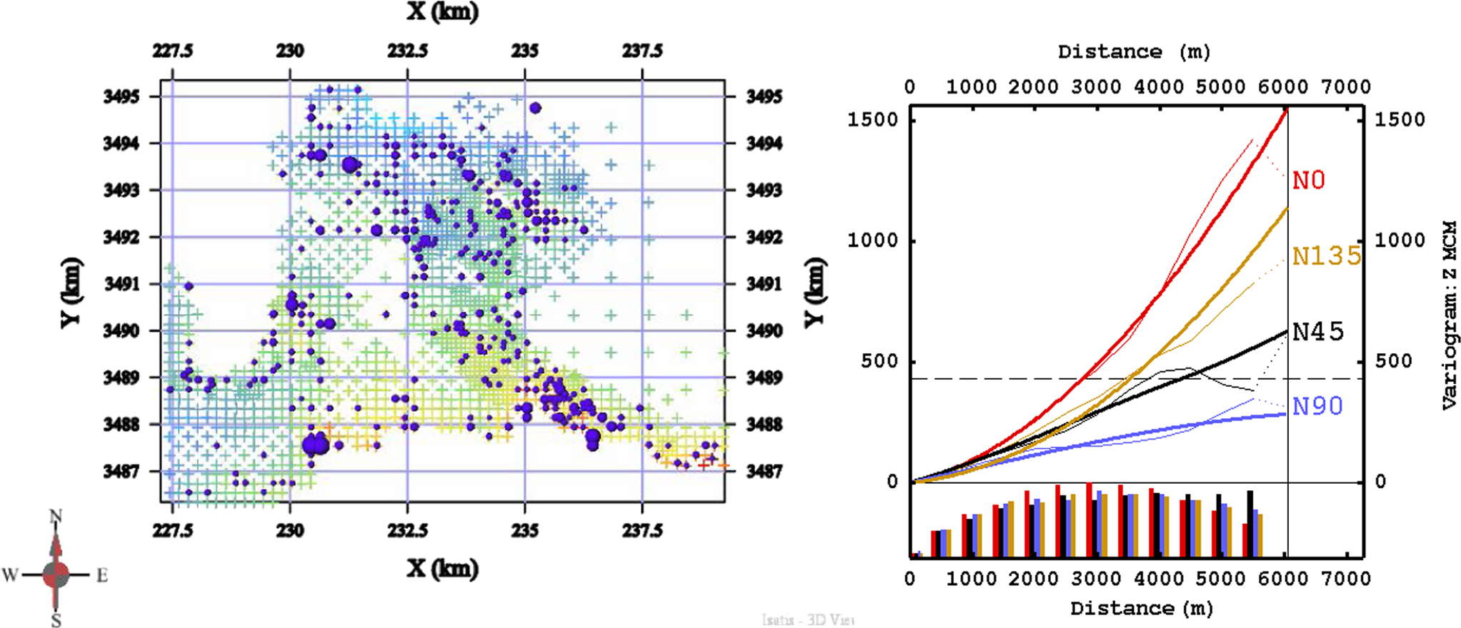
The modelling of the distribution on the SMU support (50 m × 50 m × 50 cm) requires a change of support based on the variogram model of the raw data. When the distribution is skewed, the variogram of the Gaussian transforms is modelled first; then, it is back-transformed into the variogram of the raw data by means of the Gaussian anamorphosis function (Fig. 12).
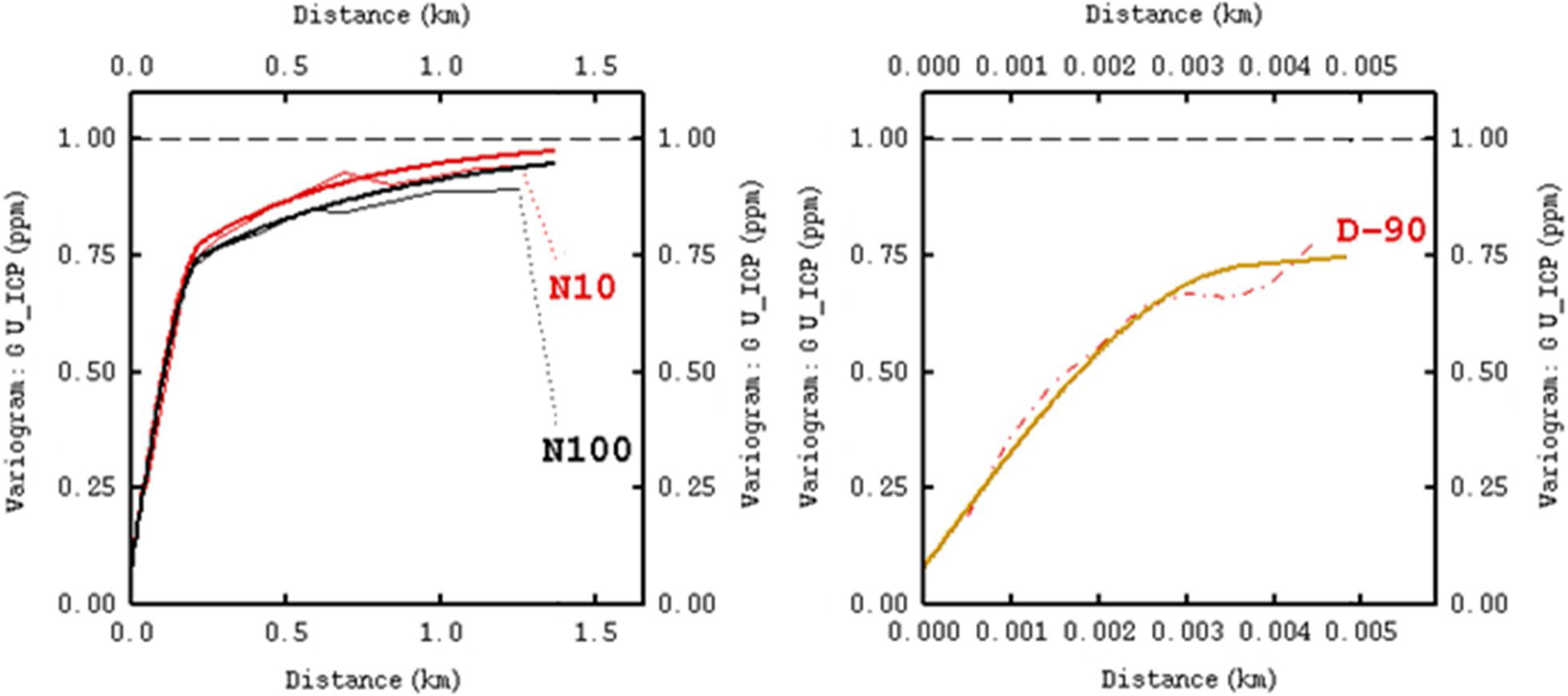
Variograms in different directions of the Gaussian transforms of U_ICP (the double line is for the model)
The support correction yields a change of support coefficient ‘r’, which measures the correlation between point and block values in Gaussian space; the lower the coefficient, the bigger the change of the block grade distribution compared to the grade distribution of composites (Fig. 13).
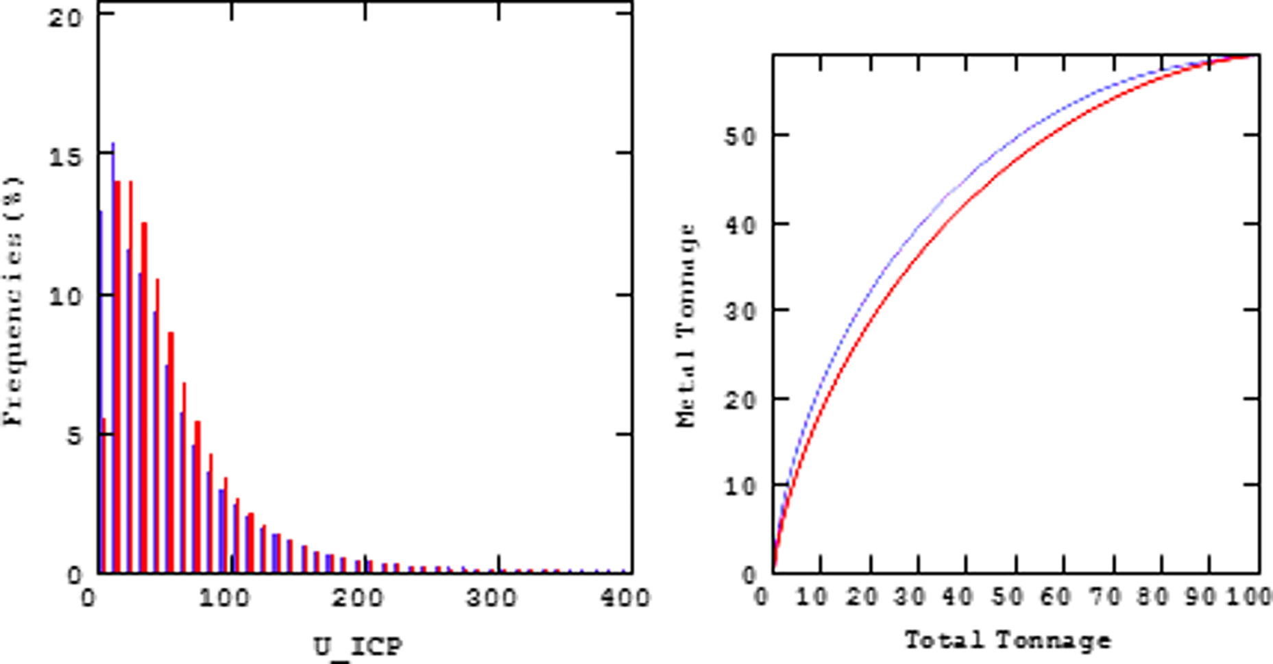
Grade distribution and metal quantity versus total tonnage on point support (blue) and selective mining unit (SMU) support (red)
UC was performed after Kriging a panel of a given height. Second grades were then distributed to each SMU of the panel so as to maintain the UC grade tonnage curves. These grades were then assigned to the SMUs according to a ranking based on the Kriged SMUs: the SMUs with the highest Kriged grade receive the grade at the highest cutoff from the UC. The localization uniform conditioning (LUC) approach has some caveats that are detailed in ‘Limitations in accepting localised conditioning recoverable resources, 2014, W. Assibey-Bonsu & C. Muller’.
Figure 14 shows that the SMUs Kriged grades (in real space) are highly smoothed, indicating that the UC/LUC procedure restores the variability of the SMUs.
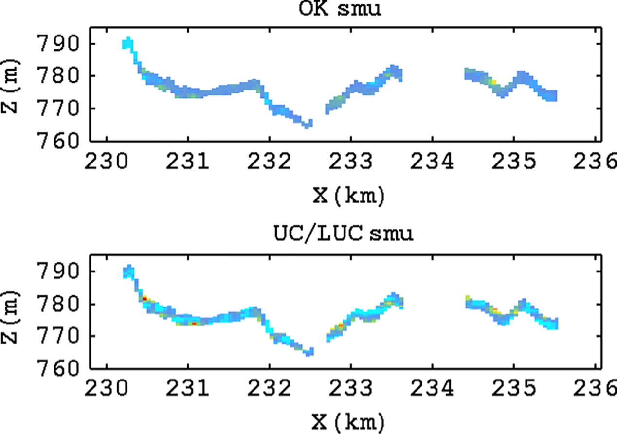
Vertical cross-section of selective mining unit (SMU) grade estimated by ordinary Kriging (OK) and by the uniform conditioning (UC)/localization uniform conditioning (LUC) procedure
A detailed examination of the block model can also be undertaken, as is shown by the swath plots in Fig. 15.
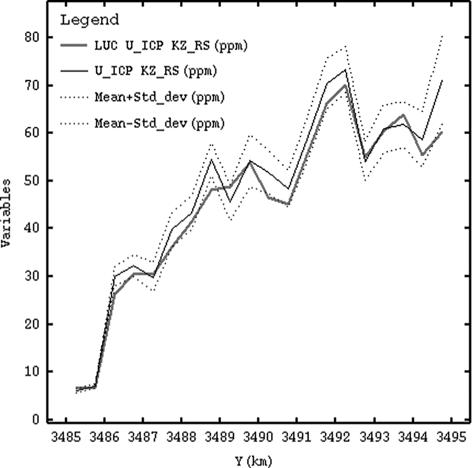
Swath plots from localization uniform conditioning (LUC) block model and composites (mean value and mean ± standard deviation) along the Y-axis
The advantage of this procedure is that the block model does not depend on an a priori decision on the cutoff grade and can be used for further calculations of the recovered resources at different cutoffs (Fig. 16).
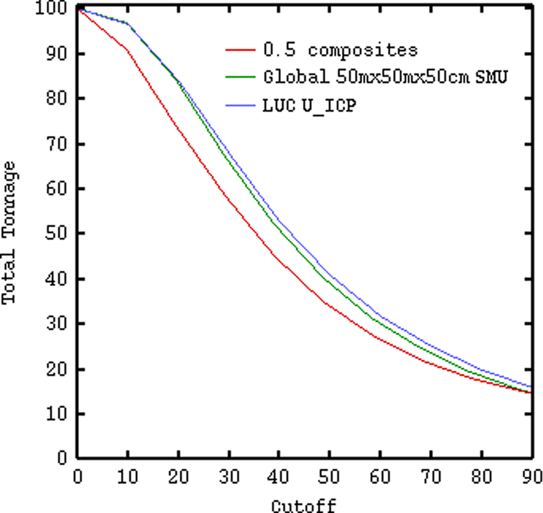
Tonnage (100% at zero cutoff) versus cutoff grade curve from the 50 cm composites (red), modelled SMU grades distribution (green) and grade SMU block model after uniform conditioning (UC)/localization uniform conditioning (LUC) (black)
Conclusion
This geostatistical study of the surficial deposits of Central Jordan has achieved its goal in that it has delivered a 3D block model conditioned to the geomorphology of the mineralisation and reflecting the selectivity that could be contemplated during production. The techniques that have been used are generally applied for more massive deposits. The possibility to adapt this approach to thinner mineralisation has also been made possible by the use of scripts within the Isatis software.
Further investigations on the trench sampling optimisation have been made and can be used as guide during the reconnaissance of other zones.
Acknowledgements
The authors are grateful to JUMCO for the permission to publish this paper based on the geostatistical study performed on the Central Jordan deposits. Thanks are addressed to Dr Marat Abzalov for the key role he played during the study.