
Abstract
The principal strategy for high level radioactive waste disposal in Sweden is to enclose the spent fuel in copper canisters that are embedded in bentonite clay ∼500 m down in the Swedish bedrock. At this depth, the groundwater is reducing. However, oxic conditions are initially established in the repository during emplacement. The corrosion rate of pure copper in an oxic bentonite/saline groundwater environment has been followed by thin electrical resistance sensors placed in a bentonite test package that was kept at room temperature for 3 years. The corrosion potentials of the sensors have verified oxic conditions in the test package. The corrosion rate of pure copper in this environment has been found to slowly decrease to quite low but measurable values; from above 15 μm/year down to ∼1 μm/year after 3 years of exposure. The measurements have verified a desired behaviour of copper in the environment.
Keywords
Background
The principal strategy for high level radioactive waste disposal in Sweden is to enclose the spent nuclear fuel in tightly sealed copper canisters that are embedded in bentonite clay ∼500 m down in the Swedish bedrock.1 The repository will be built by materials that occur naturally in the earth's crust. The idea is that the repository should imitate nature as closely as possible.
‘Nature’ has proven that
copper can last many millions of years under proper conditions: native copper has been preserved for nearly 200 million years in an environment which is similar to the repository near field environment2
bentonite clay has existed for many million years: Wyoming bentonite clay for instance was formed during the Cretaceous period, i.e. more than 65 million years ago3
the Fennoscandian bedrock shield is stable: the bedrock of interest was formed during the Precambrian period, i.e. more than 545 million years ago.4
Besides rock movement, the biggest threat to the copper canister in the repository is corrosion. The initial oxic period is considered the most harmful. It is believed that copper will last if proper environmental conditions are established and maintained.5 The most important task from a corrosion point of view is to ascertain a proper near field environment for the copper canister.
Initially, a limited amount of air will be left in a repository (and a bentonite test parcel) after emplacement, which during the water saturation phase partly will be trapped by the low permeability rim of groundwater saturated bentonite.5 After water saturation, the chemical environment in the immediate vicinity of the copper surface is determined by the composition of the bentonite pore water. This is, in turn, determined by the interaction between the bentonite and the saline groundwater in the surrounding rock. The entrapped oxygen will be consumed through reactions with minerals in the rock and the bentonite, through copper corrosion, and also through microbial activity. After oxygen has been consumed, corrosion will be controlled completely by the supply of dissolved sulphide to the copper surface.
The corrosion rate of pure copper in an oxic bentonite/saline groundwater environment has been followed by thin electrical resistance (ER) sensors for a period of more than 3 years.6 The environment was first established by pre-exposure of bentonite rings in an underground laboratory for 6 years.7 Electrochemical impedance spectroscopy (EIS) measurements have also been performed on the ER sensors and are reported elsewhere. 6 6,8
The evolution of the environmental conditions with time for a deep geological repository and their effect on the corrosion behaviour of copper have been extensively examined. 5 5,9 Recently results from ER measurements on copper exposed in bentonite and groundwater have been presented. 10 10,11 The aim of this work is to present results from corrosion monitoring of pure copper in bentonite clay saturated with saline groundwater and under oxic conditions.
Experimental
ER measurements to estimate the corrosion rate of a metal are based on the fact that a decrease in thickness of a metallic conductor causes an increase in electrical resistance.12 The sensitivity of an ER sensor is defined by its thickness; however, a lower thickness also means a shorter service life of the sensor; thus, a compromise between sensitivity and sensor life is needed. ER sensors generally do not distinguish between general and localized corrosion forms. A post-test examination of the sensors is needed to validate the result and establish the form of the corrosion attack.
Below the fabrication of the used ER sensors and their installation in the test environment are briefly described. Further information is found in Ref. 6.
Electrical resistance sensors
ER sensors are frequently used in corrosion monitoring in various fields of industrial application, such as in the petrochemical industry. In fact, the ER sensors used in the present work for corrosion monitoring of copper in bentonite are actually a modification of the sensors used for monitoring of steel corrosion in concrete.13
In the ZAG (Slovenian National Building and Civil Engineering Institute, Dimičeva 12, SI-1000 Ljubljana, Slovenia) design, thin metal foils are first hot glued on a glass fibre resin plate. Sensor and reference elements are then manufactured by a photochemical process and etched similar to printed circuits for electronic equipment. 13 13,14 The corroding sensor and reference elements are positioned in a Wheatstone bridge arrangement (Fig. 1). Pictures of sensor elements and an ER sensor are shown in Fig. 2. The reference sensor elements are protected by a glass fibre–epoxy resin plate as shown in Figure 1 Figs. 1 and 2. The soldering joints are protected by a chemical resistant elastic polymer.
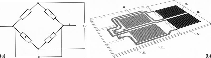
a Wheatstone bridge arrangement, and b positions of sensor (Rx) and reference (R) elements on and between glass fibre resin plates (A and B) in ZAG design
Installation of two ER sensor pairs in January 2007
In short, 35 μm thick copper foils of electronic grade oxygen free copper (C10100; min. 99·99%Cu) were first hot glued on a glass-fibre resin plate and then photochemically etched to obtain sensor elements of the form shown in Fig. 2c. The width of the electrical leads in the sensor elements is ∼0·5 mm. The nominal surface area of each one of the sensor elements is 6 cm2; thus the nominal surface area of the corroding part is 12 cm2. A direct current of 50 mA was applied for the ER measurements.
Bentonite/saline groundwater environment
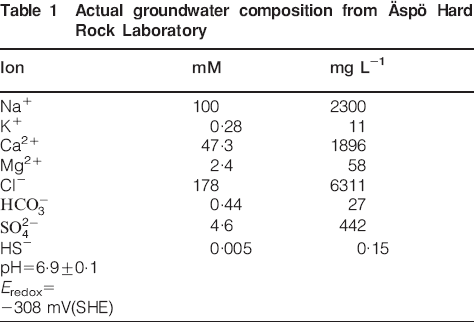
The test environment was established by pre-exposure of a bentonite test parcel in the Äspö Hard Rock Laboratory for 6 years. 7 7,15 Table 1 shows an Äspö groundwater analysis. During the pre-exposure, the bentonite rings were saturated; the target density for full water saturation was 2000 kg m−3 and the actual values fall in the range 1900-2000 kg m−3. The pre-exposure of the bentonite rings was performed at 24°C.
Actual groundwater composition from Äspö Hard Rock Laboratory
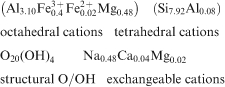
The main mineral constituent in bentonite clay is montmorillonite, which has a sheet-like crystal structure.3 As an example, Wyoming bentonite used in this study and sold under the commercial name MX-80 is dominated by natural sodium montmorillonite clay (∼80 wt-%), which is responsible for the desired physical properties. Accessory minerals are quartz (∼4%), tridymite (∼4%), cristobalite (∼3%), feldspars (∼4%), muscovite/illite (∼4%), sulphides (∼0·2%) and small amounts of other minerals and organic carbon (∼0·4%). The mean mineralogical composition of the montmorillonite part is given by:
Bentonite test package
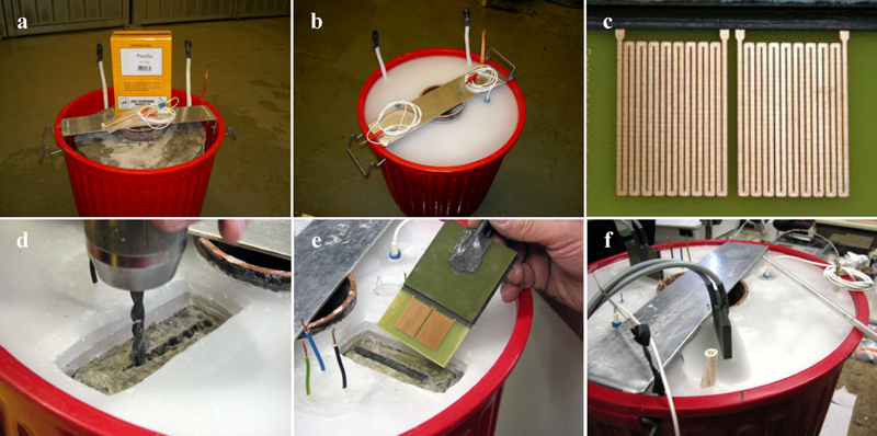
After retrieval of the above bentonite test parcel from the underground laboratory and removal of the surrounding rock, a test package consisting of three Φ30×10 cm thick bentonite rings was cut off from the test parcel with the central copper tube still in place and sealed with a thick layer of paraffin (on all sides). The top end of the copper tube is the only part of the former test parcel that is sticking out of the paraffin layer (Fig. 2). Reference electrodes to allow potential measurements were installed in the test package.
The ER sensors were installed in the bentonite test package 1 year after retrieval from the underground laboratory. They were installed in pairs with one sensor on each side of the glass fibre resin plate. Starting by drilling a row of holes in the bentonite when the paraffin layer was removed, a slot was then made in the bentonite. One side of the slot was made planar, and then wetted with Äspö groundwater before one ER sensor was placed on it, and finally the open part of the slot on the other side of the sensor pair was backfilled with bentonite borings. During the backfilling, the bentonite was repetitively wetted with Äspö groundwater. Thus, the installation procedure for the sensors on each side of the glass fibre resin plate is for practical reasons not exactly the same. Fig. 2 shows a series of pictures taken during the installation procedure and the positions of the ER sensors in the bentonite test package.
After retrieval, all measurements were performed at room temperature.
Results and discussion
In order to visualise that oxic conditions have been maintained during the exposure, and how stable the conditions have been, the recorded corrosion potentials for the ER sensors and the potential of a platinum electrode (as an estimate of the redox potential of the environment) are first shown.
The environment
Ignoring the very first period after installation of the ER sensors in the bentonite test package (when a surplus of Äspö groundwater exists on the bentonite surfaces facing the ER sensors due to wetting of the bentonite and the sensors), the corrosion behaviour of the ER sensors is governed by the composition of the bentonite pore water next to the copper surface; this has, in turn, been determined by the former interaction between the bentonite and the saline Äspö groundwater during the pre-exposure.
For the present saline groundwater and oxic conditions, the dominating corrosion stimulating species are chloride and oxygen. 5 5,16
Oxic conditions have been maintained in the bentonite test package all through the exposure. The evolution of the corrosion potential with time for the ER sensors is shown in Fig. 3. All sensors, but for the failed sensor ER2, see below, show increasing corrosion potentials with time during the period of measurement. The corrosion potentials of the copper sensors fall in the range 210-260 mV(SHE) after 3 1/2 years of exposure.
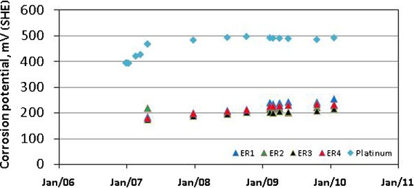
Evolution of corrosion potential with time for ER sensors compared to redox potential of environment
Performance of sensors
The ER measurements were started immediately after installation of the ER sensors in January 2007 and have regularly been performed ever since. All together more than 360 readings have been performed.
Sensor ER2 failed after an exposure of about 4 months. Sensors ER1, ER3 and ER4 have, however, survived more than 3 years of exposure. As seen from Fig. 4, a substantial part of their thicknesses has been corroded away. The estimated corrosion rate for sensor ER3 is significantly higher than for the two other survivors, ∼7 μm/year compared to ∽1 μm/year after 3 years exposure (Fig. 5). It is anticipated that this sensor and the failed sensor have experienced an uneven corrosion attack. The future post-test examination of the ER sensors will clarify this; however, post-test examination of retrieved copper coupons from the above test parcel has revealed an uneven corrosion attack, which is not due to pitting but merely an uneven distribution of general corrosion.7 Six years of exposure resulted in average corrosion rates of less than 0·5 μm/year; thus, on average only ∼3 μm of the copper surface had corroded away. However, corrosion down to a depth of 16 μm was found in one of the coupons. Similar observations have been reported earlier.17
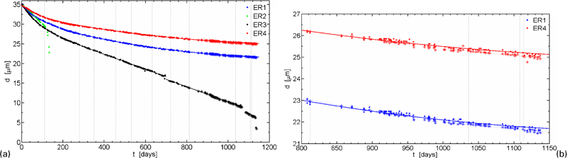
a nominal thickness change with time for four ER sensors and b comparison of primary data for sensors ER1 and ER4 (data points from two measurement systems are shown; however, only one is used for curve fitting)
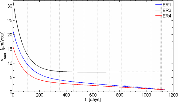
Estimated corrosion rate versus time for ER sensors
Sensors ER1 and ER4 are believed to be the most representative ER sensors in the present test for estimating the general corrosion rate of pure copper in the environment. The quality of data for these sensors is demonstrated in Fig. 4b. The technique allows measurements with a resolution as good as 0·1 μm/year.
Estimated corrosion rates
To estimate the corrosion rate during the performance of a test, uniform corrosion is assumed and a nominal corroding surface area is used as a default value for the calculations.18 An uneven corrosion attack on the corroding sensor will influence the result, but according to our experience, this is at the beginning (down to, say, 40% reduction of thickness) usually not the case. However, later on localised corrosion attack may overcome the uniform corrosion.
Nominal thickness change with time
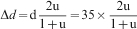
For the used sensor elements the cross-sectional area of the electrical lead A = dw, where d is the thickness and w the width of the electrical leads. The original thickness d and width w of the electrical leads were 35 μm and ∼0·5 mm respectively. Ignoring the change in width of the leads during exposure, the decrease in the sensor thickness with time can be estimated by the formula
The change of nominal thickness with time for the four ER sensors is shown in Fig. 4a and in more detail in Fig. 4b for sensors ER1 and ER4 (the vertical lines in Figure 4 Figs. 4 and 5 indicate when EIS measurements were performed8).
Given the lack of information from the post-test examination (testing is still in progress), the interpretation of the data and estimation of the corrosion rates should be considered as tentative.
Tentative estimation of corrosion rate
The evolution of the estimated corrosion rates from the time dependences of the thickness change is shown in Fig. 5. At start of exposure, the corrosion rates were higher than 15 μm/year and with time the corrosion rates have slowly decreased to quite low but still measurable values. A wide scatter of the initial corrosion rates is observed, which most probably is a consequence of the installation procedure. It is obvious from Fig. 4b that the increased corrosion rate for sensor ER1 compared to sensor ER4 during the first years of exposure resulted in 3 μm additional corrosion depth.
Also the EIS measurements have provided measurable and decreasing corrosion rates during the exposure.8 Estimated corrosion rates fall in the range 0·4-0·7 μm/year, thus somewhat lower compared to the 1 μm/year from the ER measurements.
Both the ER and the EIS measurements have supplied low but measurable corrosion rates, but higher than gravimetrically estimated average corrosion rates. Six years of exposure of copper coupons in the above bentonite test parcel at Äspö resulted in average corrosion rates of less than 0·5 μm/year; thus, on average only ∼3 μm of the copper had corroded away.
Conclusions
Corrosion monitoring of pure copper in bentonite clay has been performed. The potential measurements have verified that oxic conditions have been maintained in the bentonite test package all through the exposure.
The following observations can be made from the exposure of the pure copper ER sensors in the oxic bentonite/saline groundwater environment:
Decreasing corrosion rates through the whole exposure period (from above 15 μm/year at the start down to ∼1 μm/year at the end of exposure).
The resolution of the ER measurements was as good as 0·1 μm/year.
The ER measurements have verified a desired behaviour of copper in the environment.
A wide scatter of the initial corrosion rates, which most probably is a consequence of the installation procedure.
A possible localisation of the corrosion attack appeared on at least two of the sensors, yet to be confirmed by the post-test examination.
The results obtained from the ER and EIS measurements under the very same conditions are fairly comparable. The stability and resolution of the ER sensors have been outstandingly high. In order to improve the correlation between the two techniques, an in-depth analysis supported by information from the post-test examination of the sensors is needed.
Footnotes
Acknowledgements
This work was sponsored by the Swedish Nuclear Fuel and Waste Management Co. (SKB). C. Lilja and L. Werme at the SKB Head office in Stockholm, the staff at the Äspö Hard Rock Laboratory, and O. Karnland and his colleagues at Clay Technology AB in Lund are gratefully acknowledged for their contributions.