
Abstract
This paper presents an artificial neural network based solution method for modelling the pitting resistance of AISI 316L stainless steel in various surface treated forms. Surface treatment is a promising technique for improving the corrosion resistance of stainless steels. In this study, cyclic polarisation tests were performed before and after surface treatment. Experimental results were modelled by the neural network. The artificial neural network model exhibited superior performance based on the fitness of the observed versus predicted data. The results showed that the predicted data from the neural network model were considerably similar to the experimental data. The model has been saved and can easily be used to predict the corrosion in different surface treatment methods.
Introduction
The successful applications of stainless steels originate from the satisfactory combination of excellent mechanical properties, availability at a low cost and high corrosion resistance. Although stainless steels have high corrosion resistance in many environments, their localised corrosion can occur in certain environments.1 The superior pitting corrosion resistance of stainless steels depends significantly on the protective passive oxide layer formed on its surface.2 – 4 The pitting resistance of stainless steels is related to the formation of an insoluble, relatively unreactive chromium oxide hydroxide enriched passive surface film that is naturally formed in the presence of oxygen (self-passivation). The passive layer must be uniform, non-porous and self-healing to optimise corrosion protection. 5 5,6 Surface treatment is a technique for improving the corrosion resistance of stainless steels by forming a protective passive film. Several authors have studied the effect of surface treatment on the corrosion resistance of stainless steels. This depends on surface treatment parameters.7 – 12
The artificial neural network (ANN) is one of the most effective modelling techniques for modelling practical problems. The neural network method is now almost a standard modelling technique based on a statistical approach. In the past few years, there has been a constantly increasing tendency for ANN modelling in the different fields of material sciences.13 – 19 Most of the predictive models used to date are the regression models, which fit the data available such that their mean square error can be minimised. However, these models have been found to be effective only in very restricted areas and to be limited to capture the non-linear nature of the corrosion processes.13 – 19 The study of neural networks is an attempt to understand the functionality of a brain. Essentially, ANN is an approach to artificial intelligence, in which a network of processing elements is designed. Compared with the traditional pattern recognition, ANN can provide an accurate description for multidimensional and non-linear problems.19 The fundamental unit of ANN is the neurons, which are arranged in layers and categorised as input (I), hidden (H) and output (O) neurons, depending on which layer they are located in. As a non-linear technique, the ANN modelling involves linking up the input and output data through a particular set of non-linear basic functions.19 The procedure of ANN modelling is usually within the following contents:
artificial neural network parameter selection
data collection
database preprocessing
artificial neural network training
These steps were, necessarily, followed in the ANN model development in this paper.
The influence of surface treatment parameters on the pitting resistance of AISI 316L stainless steel has not been modelled until now. Thus, the aim of the present study was to investigate and model the influence of the surface treatment on the pitting resistance of AISI 316L stainless steel using ANNs. The treatment parameters studied in this work are nitric acid and hydrofluoric acid concentration, temperature and time. As the pitting resistance is a function of protection and pitting potentials, these two parameters were investigated to evaluate the pitting resistance.
Experimental
Specimen preparation
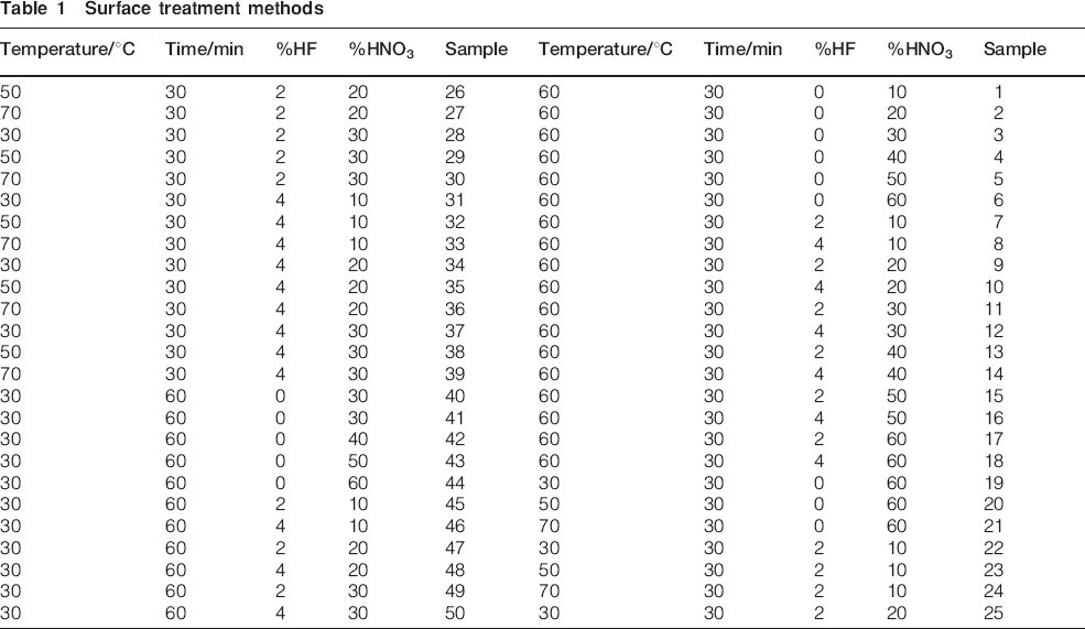
Type 316L stainless steel was used in this study. The chemical composition of this alloy, 0·031C–0·499Si–1·393Mn–0·029P–0·012S–16·810Cr–2·138Mo–9·788Ni–0·036Al–0·027Cu–0·240Co–0·009Nb–0·004Ti–0·027V–0·017W–70·160Fe (mass-%), has been obtained from quantometer method. Different surface treatments were used in this study, which can be seen in Table 1 (using 65 wt-% nitric acid and 50 wt-% hydrofluoric acid and different volume percentages). All samples before surface treatment were polished, and then each sample was degreased in ethanol and hot alkaline solution.
Surface treatment methods
Cyclic potentiodynamic polarisation measurements
Cyclic polarisation measurements were performed in a standard three-electrode cell with saturated calomel electrode reference electrode and platinum counter electrode by μAUTOLAB type III instrument. The electrodes were sealed in epoxy resin (with exposed surface area of 1 cm2). The electrochemical measurement was performed at the open circuit potential in 37°C Ringer's physiological solution with the following composition: 9·0 g L−1 NaCl, 0·17 g L−1 CaCl2.2H2O and 0·4 g L−1 KCl (ASTM.F2129). This solution was buffered with NaHCO3 with a concentration of 2·1 g L−1 and maintained the normal physiological pH at 7·4. The solutions were continuously deaerated with purified nitrogen. Corrosion measurements consisted of stabilising the working electrode in the corrosion test electrolyte at open circuit potential for 1 h with a scan rate of 0·2 mV S−1.
Artificial neural network modelling
Network architecture
The numbers of hidden neurons are chosen based on a trial and error procedure. However, the optimum number is determined by the actual training effect. In order to find the desired one, the number of neurons was varied in the hidden layers. Networks with one and two hidden layers were also investigated. A feed forward structure is a network composed of an input layer, one or more hidden layers and one output layer. Each layer consists of units or neurons. The configuration of layers and units in a neural net is called network architecture. In each layer, units receive their input from the preceding layer's units and send their output to units in the subsequent layer. In each unit, the weighted sum of its inputs is passed through the activation function to produce the output of the neuron. In this work, the non-linear hyperbolic tangent activation function (equation (1)) was used in the hidden and output layers. In a feed forward structure, no feedback loops exist; thus, the output of any layer does not affect the same or preceding layer20
Network training
In neural networks, a training set is used to learn the patterns present in the data through a training process by means of a training algorithm. The objective of training is to find the set of weights between the neurons that determine the global minimum of error function. This process is equivalent to fitting the neural network model to the available training data. Training the network with an appropriate method is the key factor in order to get a well trained network. Often, the well known back propagation method is used to train ANNs, in which the gradient is computed for a non-linear multilayer network. Therefore, in this study, back propagation training was used. In as much as such an algorithm is usually both inefficient and unreliable, it requires much iteration to converge if it converges at all. 19 19,20 In this study, 22 samples were used as training set; therefore, the Levenberg–Marquardt standard back propagation training algorithms were employed.
The Levenberg–Marquardt algorithm is one of the most popular algorithms, which is the fastest training algorithm for networks of moderate size.20
The neural network can be easily overtrained, causing the error rate on new unseen data to be much larger than the error rate on the training data. It is therefore important not to overtrain the network. A good method for choosing the number of training epochs is the early stopping technique, in which the validation data set is used to compute the error rate for it while the network is being trained. In other words, the training process must be stopped when the error measured using an independent validation set starts to increase. This method was used in this study to prohibit overtraining the problem. One-half of the remaining data was used as the validation set, which is to be used in determining the root mean square error (RMSE) for other samples.20
Model evaluation
After the network was properly trained, it has then learned to model the function that relates the input variables to the output variables and can subsequently be used to make predictions where the output is not known. This ability is called generalisation. In this paper, the test set was used to evaluate the generalisation ability of the trained network by measuring the RMSE and R 2 of the predicted data by model versus measured output data.
Results and discussion
The knowledge of the surface treatment methods in different conditions would allow the optimisation of the processing parameters in order to achieve the desirable conditions. Experimental investigation is both costly and time consuming. Based on trained neural networks, a model for simulation pitting corrosion was created. The data set was constructed by collecting 50 experimental tests for different surface treatment conditions. In this study, an ANN model is presented for the prediction of pitting corrosion in 316L stainless steel as a function of surface treatment variables.
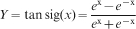
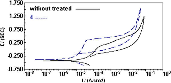
The pitting or critical potential E b and the protection potential E p for every specimen were evaluated by the cyclic potentiometer method in Ringer's solution. Figure 1 Figure 2 Figures 1-3 show the cyclic polarisation curve in Ringer's solution for untreated and surface treated samples at different conditions. The influence of acid concentration and temperature on surface treatment was compared in Figure 2 Figs. 2 and 3. The dependence of E p and E b on acid concentration is shown in Fig. 4. It is clear that both E p and E b increased with increasing nitric acid concentration up to the range of 20-30 wt-%, and then E p and E b decreased with increasing acid concentration because over this range, the film formed on the surface layer is soluble in the acid and is not protective. Another important parameter that may affect the pitting resistance of surface treated stainless steel is the temperature. Figure 5 shows the pitting potential of 316 stainless steel at different temperatures. The pitting resistance is proportionate to temperature up to 70°C and then decreased with increasing temperature. At higher temperature, the pitting resistance is decreased because the surface layer is not protective at higher temperatures. It has also been claimed that at higher temperatures, it can result in the so called overpassivation, which may increase the corrosion potential considerably and therefore increase the risk for pitting corrosion attacks. These results were used for constructing the dataset for ANN modelling considering the main factors, which were the concentration of nitric and hydrofluoric acid, temperature and time.
Cyclic polarisation curve in Ringer's solution for surface treated and untreated sample
Cyclic polarisation curve in Ringer's solution for samples 4, 6, 10 and 14
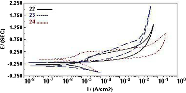
Cyclic polarisation curve in Ringer's solution for samples 22, 23 and 24
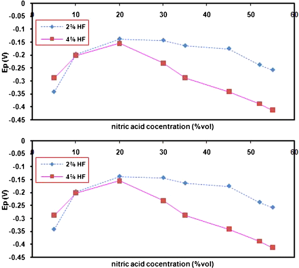
Dependence of E p and E b on acid concentration
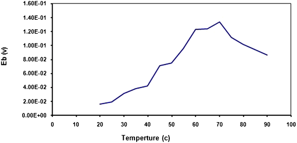
Pitting potential of 316 stainless steel at different temperatures
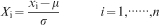
The performance of an ANN model depends on the data set used for its training. The available data were divided into three groups: 40% for the training set, 30% for the validation set and 30% for the test set. The input data (concentration of nitric and hydrofluoric acid, temperature of surface treatment solution and time) and the output data (the pitting and protection potential) were normalised to be in the range from −1 to 1, with a mean of 0 and standard deviation of 1 (equation (2)), where X i represents the ith data, and μ and σ are mean and standard deviations of the data respectively. One of the problems that occurs during neural network training is overfitting. The error on the training set is driven to a very small value, but when new data are presented to the network, the error is large. The network has memorised the training examples, but it has not learned to generalise to new situations.20 To avoid ANN overtraining, the ‘early stopping’ method was used. Whenever the mean square error of evaluating the set began to rise, the training process of the network would be stopped
Variation in mean square error for different network topologies
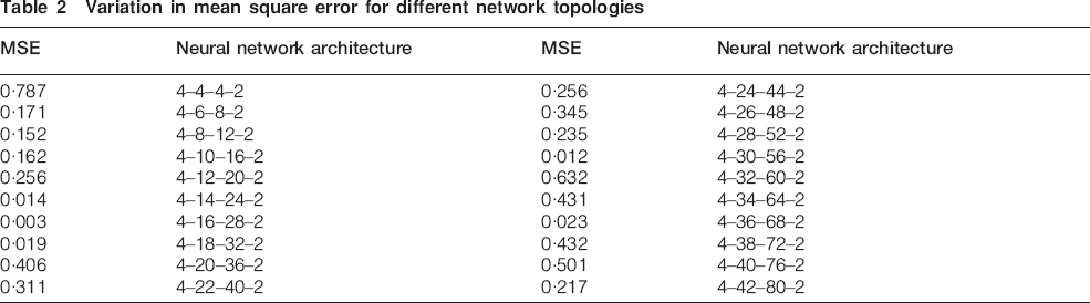
It can be seen in Table 2 that the optimum architecture was 4-16–28-2 with less mean square error.
Figure 6 shows the mean square error for training, validation and testing data during the training process for the aforementioned model.
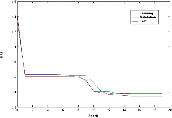
Mean square error during training process for training, validation and testing data for 4-16–28-2 network
The overall performance of the network can be verified using predicted values of the network versus measured values. The scattered plots of these values are shown in Fig. 7. It can be seen that the model prediction fits well with the experimental observation. The developed network shows good performance, and the network results are in good agreement with experimental data.
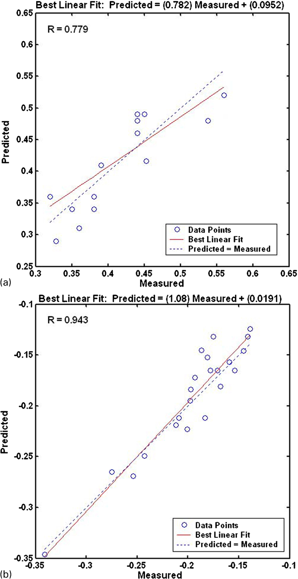
Scattered plots of predicted against experimental data
In as much as the experimental data in this study were distributed uniformly in an almost wide range of different situations, including the upper and lower limits of surface treatment conditions, the model can be considered robust enough to be used for prediction. This was concerned due to the fact that the neural networks are inherently successful to be used for the interpolation of data, and normally, extrapolation by ANN does not yield a good result.
The optimum model, which was 4-16–28-2, was then saved to be used for further prediction of pitting and protection potential.
Conclusions
The influences of surface treatment on pitting and protection potentials are difficultly described by simple mathematics equations because of the intricate relation between input factors. The ANN models in such cases can serve as a favourable alternative for prediction instead of complicated calculations.
The effect of the concentration of nitric and hydrofluoric acid, temperature and time on the pitting resistance of 316L stainless steel alloy was modelled by means of ANNs. The optimal ANN model architecture of 4-16–28-2 was considered as a suitable model for the prediction of pitting and protection potentials of surface treatment on stainless steel.
A promising agreement between experimental and predicted data for the developed model confirmed its effectiveness for corrosion prediction.