
Abstract
Carbon steel is commonly used in Mauritius, and information related to its atmospheric corrosion behaviour in the Mauritian atmosphere is not readily available. Hence, the present study was performed to obtain relevant data and to develop a model for predicting the atmospheric corrosion degradation of carbon steel in Mauritius. Carbon steel samples were exposed outdoors at several sites, according to BS EN ISO 8565. They were removed after specific time periods, and their mass loss was determined. At the same time, the sites’ environmental parameters were monitored. From the mass loss measurements and the environmental parameters considered, it was found that the corrosivity of the Mauritian atmosphere falls in category C3 to C4, according to ISO 9223. A model was developed using the SPSS software, and it was found that the atmospheric corrosion in Mauritius depends mainly on the time of exposure and the carbon content of carbon steel.
Introduction
In Mauritius, there is an increasing use of carbon steel, especially in the fabrication of structures, such as steel buildings. However, basic information concerning its resistance to atmospheric corrosion in the Mauritian atmosphere is not readily available.
Mauritius is a small tropical island of 1865 km2, located in the Indian Ocean, as shown in Fig. 1.1 Taking into consideration its size and location, airborne salinity is expected to be quite high. In fact, extremely high level of sea salt fallout of 0·3-0·45 kg/m2/year has been recorded on oceanic islands and coastal areas.2 Moreover, the relative humidity in Mauritius is frequently >80%. Hence, the actual time during which the metal surface remains wet, that is, the time of wetness (TOW), can be very high. This high level of relative humidity coupled with a high level of airborne salinity can enhance the atmospheric corrosion effects,3 and they are expected to contribute to the serious atmospheric corrosion problem actually prevailing in Mauritius. The present study was therefore performed in order to get a better insight into this problem.
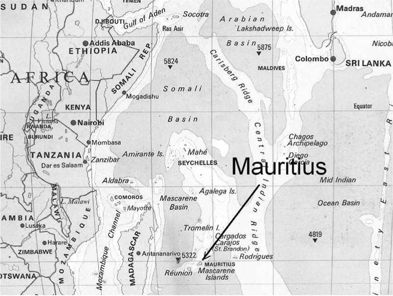
Location of Mauritius in Indian Ocean
Investigations on the atmospheric corrosion behaviour of carbon steel in different types of environments have been generally performed through outdoor exposures and weight loss analysis. Outdoor exposures have been performed in various tropical countries worldwide. Large corrosion losses, falling in the corrosion category C4 and C5, according to ISO 9223,4 have been reported in the tropical regions of Mexico,5 India6 and Vietnam.7 Mauritius, being a tropical island, is also expected to experience similar atmospheric corrosion degradation.
Relative humidity, airborne salinity and pollutants, such as sulphur dioxide, have been found to be the main factors that affect the corrosion rate in the tropical regions.8 As already mentioned, relative humidity affects the TOW, which, on its side, directly affects the time during which atmospheric corrosion takes place on the metal surface. From the atmospheric corrosion tests performed in the tropical humid climate of the Yucatan Peninsula,5 in Mexico, it was recommended that in such types of climates, corrosion should be expressed as a function of the TOW. Airborne salinity can be developed by the ocean and the surf at the shoreline and is transported inland in the form of salt aerosol. It has been found to be a major cause of atmospheric corrosion in Australia.9 Similar results have been obtained in other studies worldwide.10 – 12 Sulphur dioxide, on the other hand, is regarded as a powerful atmospheric corrosion stimulator,13 and together with salinity and relative humidity, it is considered as a major factor affecting the atmospheric corrosion.14 Meteorological parameters, angle of exposure, height of the exposed samples and types of samples are among the other factors that can affect atmospheric corrosion.
Atmospheric corrosion tests are nowadays performed not only to characterise the corrosivity of an atmosphere but also to predict the effect of corrosion on the metal. For carbon steel, various types of models have been developed for this purpose.
The widely accepted simple model for long term atmospheric corrosion of steel conforms to an equation of the form15,16

Guttman and Sereda,17 on the other hand, studied the mass loss on metals due to corrosion and causative environmental factors, namely, TOW, panel temperature, atmospheric sulphur dioxide and airborne salinity, at four inland and three coastal North American test sites. Simple empirical equations were then developed based on regression analysis and curve fitting techniques for finding material loss. One such equation of the following form for steel, copper and zinc was proposed
Recently, holistic models have been commonly developed and used. Graedel and Leygraf18 proposed a procedure to predict the expected corrosion damage rate using dose response functions. The approach is based on the ‘dose response’ relationships for materials. In these types of models, the rate of corrosion is termed ‘response’, and the atmospheric corrodant is termed ‘dose’. Mathematically

The GILDES computer models have also been developed to predict atmospheric corrosion damage.18 In the GILDES models, six distinct regimes are considered: the gas phase (G), the interface between gas and liquid (I), the thin liquid layer (L), the deposition regime containing the corrosion products (D), the electrodic layer (E) and the surface/solid (S).19
Today, other types of models using artificial neural network (ANN) are being used to fit environmental variables with the corrosion rates of metals. The ANN is expected to give better results, for the damage function of metals, than traditional linear models. It is excellent for modelling non-linear and complex systems and can interpolate from past experience. It can be seen as a ‘super-regression’ technique and tends to be fault tolerant and can therefore be used to model atmospheric corrosion processes.20
The present study is aimed to bring some light on the problem of atmospheric corrosion in Mauritius through the outdoor exposure of carbon steel samples. The corrosion behaviour of carbon steel would be studied, and the corrosivity of the Mauritian atmosphere would be determined. This would be consolidated by the development of a model for atmospheric corrosion in Mauritius using regression analysis, which can be used to estimate and predict atmospheric corrosion in Mauritius.
Experimental
Two types of commercially available carbon steel samples, which would be henceforth referred to as types A and B samples, were exposed outdoors at six sites, in Mauritius, according to BS EN ISO 8565.21
For type A samples, three sites were chosen:
Reduit: it is found in a rural region, 9 km from the nearest coast, and very near to industrial zones and the other towns
Vacoas: this site is found in an urban region, 13·5 km from the nearest coast
Palmar: it is found in a rural region, very far from sources of heavy pollution, but near the sea shore (500 m inland).
For type B samples, four sites were chosen:
Reduit: same site as above
Belle Mare: it is situated on the eastern coast of Mauritius, 50 m from the shore line; this is a purely marine site, far away from industrial and urban regions
Port Louis: this site is found at the shoreline and in the capital city
St Julien d'Hotman: this site is found far away from the industrial and urban regions and can be regarded as a rural site, 16 km inland.
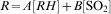
The sites chosen are shown in Fig. 2.1 They were chosen so that there is a good mixture of the different types of atmosphere commonly found in Mauritius. This would also be helpful while producing the model for atmospheric corrosion loss.
Map of Mauritius showing sites at which metal samples were exposed
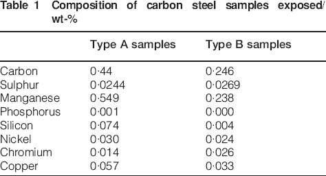
The two types of carbon steel samples chosen vary in their composition. This variation would also help the modelling proposed in the paper. The composition (wt-%) of the main alloying elements in the carbon steels used is shown in Table 1.
Composition of carbon steel samples exposed/wt-%
Both types of samples were cleaned and polished before exposure, and their surfaces showed an average three-dimensional mean roughness of 1·4 μm. Type A samples were removed in sets of 3 at approximate intervals of 1·5, 3, 6, 9, 12, 15 and 18 months for mass loss determination. Type B samples were, on their side, removed in sets of 4 at approximate time intervals of 2·5, 7, 12 and 19 months. Additional samples were retrieved from the exposure racks for each of the removals. These samples were cut to the required size for the topographical analysis of the rust layer through the scanning electron microscope (SEM). Simultaneously, the level of airborne salinity was monitored through the wet candle method.22 The tests were performed twice annually, i.e. in the summer and winter seasons. Sulphur dioxide levels were obtained from mobile monitoring stations performing pollution level monitoring throughout the exposure period. The atmospheric parameters were obtained from the stations of the Mauritius Meteorological Services. The parameters obtained were then averaged over a daily period for the exposure period of the samples considered.
When the samples were removed after exposure, they were cleaned for determining the mass loss. This consisted of light mechanical cleaning to remove loose corrosion products followed by chemical cleaning according to BS 7545.23 The samples were cleaned in a sodium hydroxide solution to which zinc was added at 85°C for 30 min.
After cleaning, the mass loss of the samples was determined, and the corrosion loss (in μm) was then calculated. This was used for corrosivity categorisation of the sites considered.
The environmental parameters monitored together with the corrosion loss determined through mass loss analysis were then used to develop the model for atmospheric corrosion prediction.
Results and discussion
Mass loss analysis and corrosivity
The mass loss obtained for the samples were converted to corrosion loss (in μm) so as to get a clearer view of the corrosion damage on the metal. The results of corrosion loss against days of exposure for the all the sites are shown in Fig. 3.
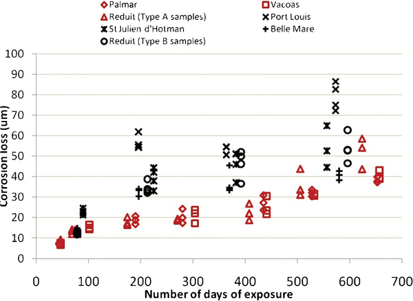
Results of corrosion loss against time of exposure
As already discussed, it is widely accepted that atmospheric corrosion of carbon steel normally conforms to equation (1). Hence, the results at the sites considered were modelled according to equation (1). The equation of the trend curve, for each site, and the respective coefficient of determination (R 2 value) are shown in Table 2. From the high R 2 value obtained, it can be deduced that equation (1) represents well the corrosion behaviour of carbon steel in Mauritius.
Equation of trend curve for corrosion of carbon steel
For type A samples, the b value is near to 0·5, which suggests that the corrosion reaction is diffusion controlled. For type B samples, the b value for Port Louis is equal to 0·89, which is very high and suggests that the rust layer was loosely adherent, which resulted in an increase in the corrosion reaction. Much flaking of the rust layer was, in fact, observed on the samples. For Belle Mare and St Julien d'Hotman, the b value was near to 0·5, which suggests a diffusion controlled corrosion reaction. At Reduit, the corrosion reaction was proceeding at an accelerating rate. It could also be observed that the corrosion loss in type A samples was generally lower than that of type B samples.
For each of the sites, the equation obtained in Table 2 was used to determine the corrosion loss of the samples over a 1 year period, and this was compared with ISO 92234 for determining the corrosivity of each site. It was found that
Port Louis falls in category C4, which refers to an environment with high corrosivity
Palmar, Reduit and St Julien d'Hotman fall in category C3, which refers to an environment with medium corrosivity
Vacoas falls in category C2, however, very near to the borderline between categories C2 and C3.
Hence, taking into consideration that the different types of atmospheres in Mauritius have been considered in this study, it can be deduced that, generally, the corrosivity of the Mauritian atmosphere would lie in category C3, with the exception of Port Louis, where the corrosivity would lie in category C4.
Scanning electron microscopy
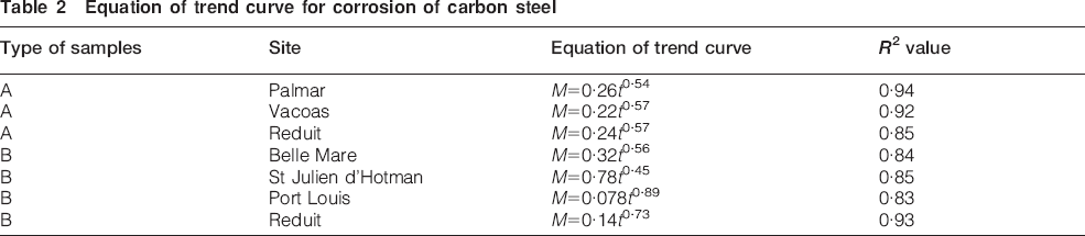
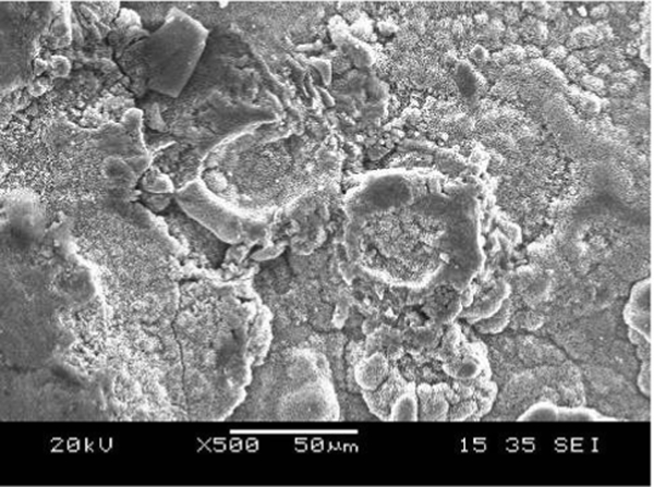
From Fig. 3, it can be deduced that the atmospheric corrosion rate is high initially (for the first 3 months), and it decreases considerably with time. This is confirmed from the SEM images obtained.
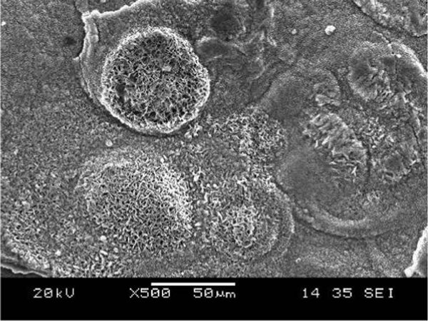
A typical variation of the rust topography is shown in Figs. 4 7. From Figs. 4 and 6, it can be observed that the micrographs of Reduit (type A samples) and Port Louis (type B samples) clearly show the formation of a porous rust layer, which leads to a high initial corrosion rate. It grows thick with time, and the corrosion rate decreases. Eventually, cracks are formed, as observed in Figs. 5 and 7, which keeps the corrosion rate at a significant value.
Images (SEM) for samples collected at Reduit (type A samples) after second removal (69·1 days of exposure)
Images (SEM) for samples collected at Reduit (type A samples) after fourth removal (271·1 days of exposure)
Images (SEM) for samples collected at Port Louis (type B samples) after first removal (80·1 days of exposure)
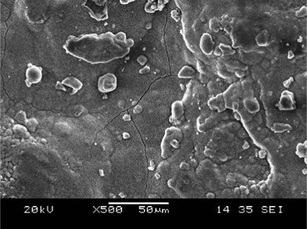
Images (SEM) for samples collected at Port Louis (type B samples) after third removal (364 days of exposure)
Environmental parameters
Sulphur dioxide, airborne salinity and TOW
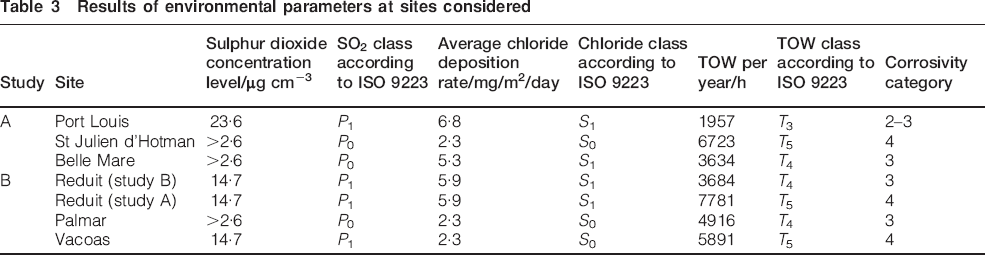
Much variation was not observed for the sulphur dioxide and airborne salinity levels. Mauritius is highly ranked in terms of air quality, and this shows in the results obtained. Table 3 shows the sites considered and the 24 h average concentration level of sulphur dioxide over a yearly period and its corresponding class, according to ISO 9223.
Results of environmental parameters at sites considered
As for airborne salinity, it can be transported in the form of salt aerosol,9 which can be generated by:
the ocean, through bursting bubbles generated by ocean whitecaps
from the surf at the shoreline, through breakers on the shore.
The amount of salt produced by the ocean is relatively constant inland. The salt produced at the shoreline, normally, shows an exponential decrease with distance from the coast.24 In Mauritius, the sea is very calm due to coral reefs surrounding the island, and the wind speed is quite low, with averages of 3-4 m s−1 in many areas. Moreover, the beaches consist of very effective wind barriers in the form of coniferous trees and other types of vegetation. These situations, consequently, result in a low level of airborne salinity that decreases rapidly while moving inland. The yearly average airborne salinity level at the sites considered is as shown in Table 3.
The TOW, calculated from the daily relative humidity and temperature variation, according to ISO 9223,4 is as expected for a tropical country. Table 3 shows the TOW categorisation for each site. The TOW at Reduit is not the same for the two types of samples because they were initially exposed at different times.
Corrosivity category according to environmental parameters
Taking into consideration the environmental classifications of the sites, their corrosivity was obtained, according to ISO 9223,4 as shown in Table 3.
It can be observed that the corrosivity at the sites considered varies between categories C3 and C4. The result for Vacoas has been found to be significantly different from that obtained through the mass loss analysis. Discrepancies using the different methods of classification have also been observed for Port Louis, St Julien d'Hotman and Reduit (type A samples). These types of differences have been observed by other researchers in their respective studies, and it has been pointed out that the environmental parameters taken into consideration in ISO 9223 are not adequate for corrosivity classification.25 Factors that could have influenced the results are, first, the method of calculating the TOW, which is not suitable for coastal regions in tropical countries.26 Second, other factors such as material composition have not been thoroughly considered in the ISO 92234 classifications.5 Still, it can be deduced that the atmosphere in Mauritius would normally fall in category C3 to C4.
Atmospheric parameters
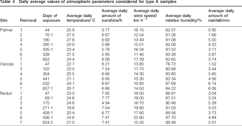
The atmospheric parameters that were collected for developing the model, that is, temperature, sunshine, wind speed, relative humidity and rainfall, are shown in Tables 4 and 5. It can be observed that the average daily relative humidity for Port Louis is the lowest of all the sites. Still, it is >70%. At the other sites, the average daily relative humidity is higher and is even >80% in many cases.
Daily average values of atmospheric parameters considered for type A samples
Daily average values of atmospheric parameters considered for type B samples
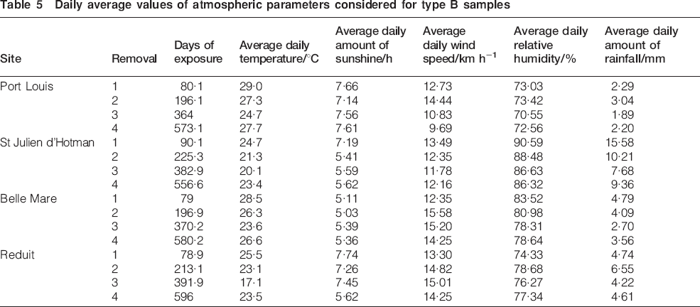
Temperature and rainfall vary according to seasonal changes. However, it can be observed that the coastal sites (Port Louis, Palmar and Belle Mare) are hotter than the rest. Port Louis has also the least rainfall.
Modelling
The model would basically be a damage function that needs to be simple and easy to use. It would therefore eventually consist of a maximum of three independent variables that can best be correlated to the dependent variable.
Multiple linear regression was be used to obtain the model. The independent variables considered were: time of exposure, atmospheric parameters, concentration of sulphur dioxide, deposition rate of airborne salinity and carbon content in the carbon steel. The corrosion loss of the carbon steel samples was taken as the dependent variable.
Statistical analysis
For study A, the samples were normally removed in groups of three, whereas for study B, the samples were removed in sets of 4. The data available, for the mass loss for the samples removed from the exposure rack at each removal, were not grouped, and there was, as a result, 123 data sets available for analysis.
Checking of distribution
There was no missing value.
Ratio of cases to independent variables: the following rule of thumb takes into account the effect size27
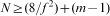
For the present analysis, the model would use at most three of the available independent variables. If f 2 is assumed to be 0·15, then N⩾54. Hence, the available sample size is large enough to at least observe large and medium effects.
Checking for outliers and normality among independent and dependent variables
For each type of variable, the distribution was checked for outliers. The presence of outliers is detected with standardised scores in excess of 3·29 (p<0·001, two tailed test) standard deviations below or above the mean.
No outlier was present. Table 6 shows the results obtained. However, the data for the average daily amount of rainfall are skewed. The kurtosis for the average daily amount of rainfall is also high. Therefore, the data for the average daily amount of rainfall is a good candidate for transformation. The data for kurtosis and skewness for carbon content were not calculated. This is due to the fact that it consists of only two values (0·44 and 0·22) for two different types of metals used for the samples. Owing to the small variation in the levels of sulphur dioxide and airborne salinity, and the synergistic effect of these two pollutants,28,29 they were grouped together, as shown in Table 6.
Checking distribution of dependent and independent variables*
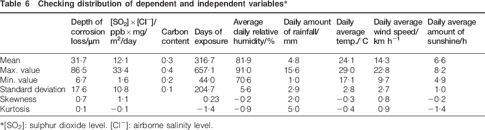
*[SO2]: sulphur dioxide level. [Cl−]: airborne salinity level.
Otherwise, the other parameters have a fairly normal distribution.
Improving data sets
The data for depth of corrosion and days of exposure were transformed for incorporating them into the equation for the model, as shown in Table 7. The data for the daily amount of rainfall were raised to the power of 0·05 to improve the normality of the distribution.
Transformation of dependent and independent parameters
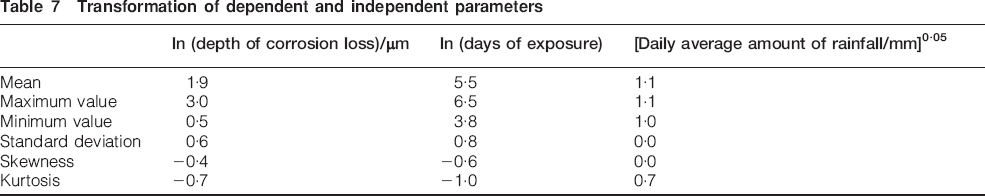
The transformation for depth of corrosion and days of exposure was necessary for the model, but this has not resulted in any significant amelioration in the normality of these sets of data. However, it can be assumed that the distribution for the respective population is normal. On the other hand, the distribution for the transformed daily amount of rainfall has shown an improvement in the normality.
For the statistical analysis using the SPSS software, the following abbreviations were used for the dependent and independent variables:
ln (depth of corrosion): LnCorros
ln (days of exposure): LnDaysOfExp
[SO2]×[Cl−]: AtmPoll
daily average relative humidity (%): RH
[daily amount of rainfall (mm)]0·05: Rainfall
daily average temperature (°C): Temperature
daily average wind speed (km h−1): WindSpeed
daily amount of sunshine (h): Sunshine
carbon content (wt-%): CC.
A sequential procedure was employed to select variables for inclusion in the regression variate. The models shown in Table 8 were initially tested.
Models initially tested
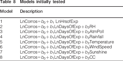
Table 9 shows the results obtained for the correlation coefficient, coefficient of determination and the maximum Mahalanobis distance. These parameters were used to choose the most appropriate model for atmospheric corrosion determination.
Results for models 1-8
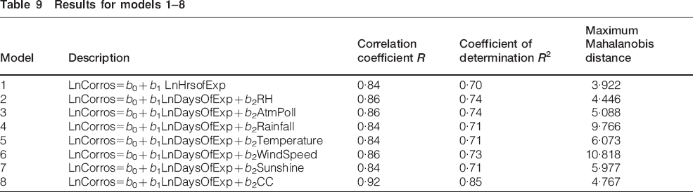
Taking into consideration the correlation coefficients, it was observed that the one for model 8 had the highest value. The Mahalanobis distance was also low, and therefore, this model was used for further analysis.
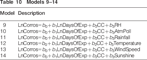
One more independent variable was added as an additional parameter into model 8 in order to obtain a better correlation. The models tested are shown in Table 10.
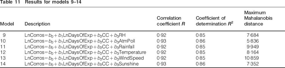
Models 9-14
The results obtained are shown in Table 11. It can be observed that the addition of a parameter has not led to any improvement for models 9, 11, 12 and 13. Models 10 and 14 have only been insignificantly improved. Moreover, there has been an increase in the Mahalanobis distance, which confirms that the additional parameter has not led to any improvement in the model.
Results for models 9-14
Hence, based on simplicity and amount of results that can be explained, model 8 is found to be the best one. However, the model has to be further assessed for its statistical soundness.
Assessing model
Apart from the correlation coefficients and the Mahalanobis distance, the following properties were therefore tested to assess the model:
normality and absence of heteroscedasticity
significance of the regression and regression coefficients
absence of multicollinearity among its variables.
Heteroscedasticity and normality
The normal probability plot, as observed in Fig. 8, shows normality in the model. From the scatterplot of the residuals, as shown in Fig. 9, it can be observed that heteroscedasticity was absent.
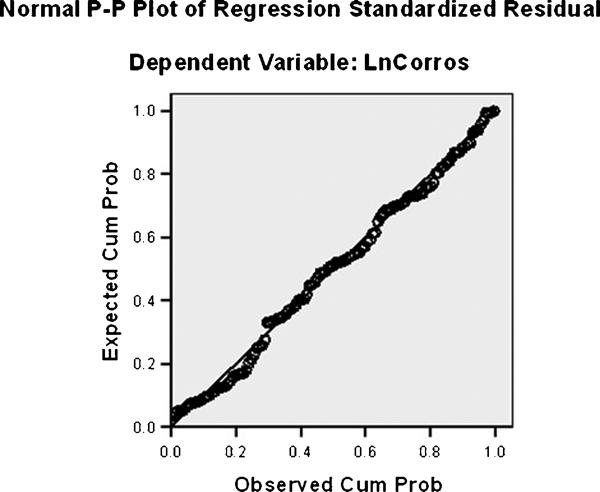
Normal probability plot for model 8
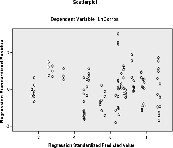
Scatterplot of residuals for model 8
Significance of regression and regression coefficients
An F test was performed to test whether the regression was significant. The theoretical value of the F ratio, with v 1 = 2 and v 2 = 120 and significance level of 0·05, was 3·0. The calculated F ratio, from SPSS, was found to be >3·0, as shown in Table 12. This implies that the regression is significant.
Analysis of variance table obtained from SPSS results for determining significance of regression*
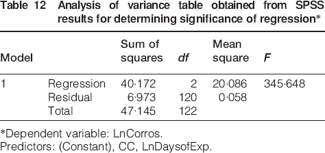
*Dependent variable: LnCorros.
Predictors: (Constant), CC, LnDaysofExp.
The t statistic was used to test the statistical significance of the regression coefficients. At a significance level of 0·05, for a two tailed test, and for 120 degrees of freedom, the theoretical value of the t statistic is 1·98. Therefore, all the regression coefficients whose calculated t statistic is numerically <1·98 would be insignificant. The main outcome of the t test is shown Table 13. All the calculated t values for the regression coefficients were numerically >1·98, meaning that they were all significant.
SPSS results for determination of significance of regression coefficients
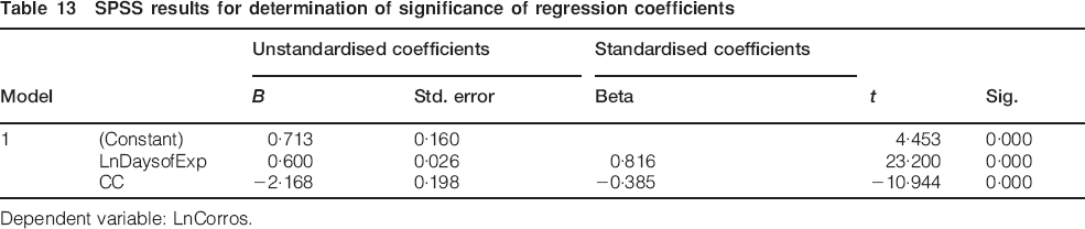
Dependent variable: LnCorros.
Multicollinearity
A condition index >30 coupled with variance proportion >0·50 would suggest the presence of multicollinearity. The SPSS results are shown in Table 14. It can be observed that for model 8, the condition index is <30, implying the absence of multicollinearity.
Checking for multicollinearity diagnostics*
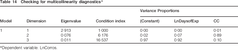
*Dependent variable: LnCorros.
Model chosen and discussion
From the tests performed, it can be concluded that model 8, as shown in equation (6), can be regarded as the best model, which is simple, easy to use and statistically correct
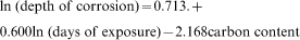
The model shows that carbon content has an adverse affect on the corrosion rate. It decreases the corrosion loss with time, and this is has been observed by other researchers.12
It can also be observed that the atmospheric corrosion degradation of carbon steel in Mauritius depends mainly on the duration of exposure of the metal in the atmosphere and the composition of the metal. The environmental parameters do not have much effect on atmospheric corrosion. One main reason for this type of behaviour is that Mauritius is a small island, and although the different sites have different environmental parameters, they do not differ significantly. Moreover, not much difference has been observed from the corrosivity categorisation of the sites considered using the environmental parameters.
Conclusion
In this study, the corrosivity of the Mauritian atmosphere was determined. The Mauritian atmosphere generally falls in corrosivity category C3 to C4, according to ISO 9223.
The model for atmospheric corrosion degradation can be represented by equation (6), and only two parameters, that is, days of exposure and carbon content, were found to explain 85% of the observations. Carbon content has an adverse effect on the corrosion degradation of the metal. The environmental parameters considered were not found to have a significant effect on explaining the atmospheric corrosion of the metal. However, other techniques, such as ANN, can be expected to improve the results.