
Abstract
The bimodal model previously shown to be applicable to long term corrosion loss of mild steel in seawater is examined herein for hard freshwater at elevated temperatures. Laboratory data reported in the literature are reinterpreted using conventional corrosion theory and the bimodal model. The data fit the trends for the parameters of the model extrapolated from water temperature observations. One different set of data earlier can be reconciled if allowance is made for the effect on corrosion of water velocity. Overall the results show the bimodal model is applicable to freshwaters to 70°C.
Introduction
Corrosion of mild steel at elevated water temperatures and in particular in hard freshwaters is of practical interest. Applications include ships operating in tropical freshwater lakes or in tropical brackish waters and storage and piping of freshwater, for example, for drinking water supplies and heating and ventilation units. Perhaps surprisingly, there appears to be very little data in the open literature for the corrosion of freshwaters at elevated temperatures.1 This was confirmed in discussions with industry experts who noted that confidential data for longer term comparative corrosion of hot water systems are held by individual companies but that these tended to be unwilling to divulge their proprietary information.
One relatively small set of data was reported by Chernov et al.2 for corrosion losses of mild steel in hard freshwater exposed in the range 50-60°C for up to 2 years in a steel storage tank in a solar heating plant in Vladivostok, Russia. There was very little water circulation and stratification of dissolved oxygen was observed. Compared to the bimodal corrosion model (reviewed briefly below) derived originally for lower temperature seawaters and also fresh waters3 some consistency could be shown with respect to the Melchers and Chernov4 data. In the present paper laboratory observations reported by Mercer and Lumbard5 for the corrosion of mild steel in hard Teddington tap water at 70°C are used, with some interpretation, to show consistency with the bimodal model. In particular consistency is shown with trends for the parameters of the model when these are extrapolated to higher water temperatures. The extrapolation is directly from parameter evaluations made for water temperatures in the range 4-29°C. Some observations are then made about the interpretation that should be placed on the Vladivostok data. It may be reconciled with the model provided allowance is made for the known effect of low water velocity of shorter term corrosion losses. As a result it is proposed that the bimodal model is applicable also to the corrosion loss of steel in waters up to 70°C.
Review of bimodal model
The bimodal corrosion model is shown in schematic form in Fig. 1. It was proposed originally for seawater immersion corrosion loss6 and may be considered as a refinement of the well known power law model used extensively in the atmospheric corrosion literature and for describing early progression of pit depth with exposure time.7 The model of Fig. 1 has been shown to be consistent with a wide range of published data both for corrosion loss and for pitting, including a variety of low alloy steels and chromium steels and for a range of exposure conditions including brackish and freshwater.8
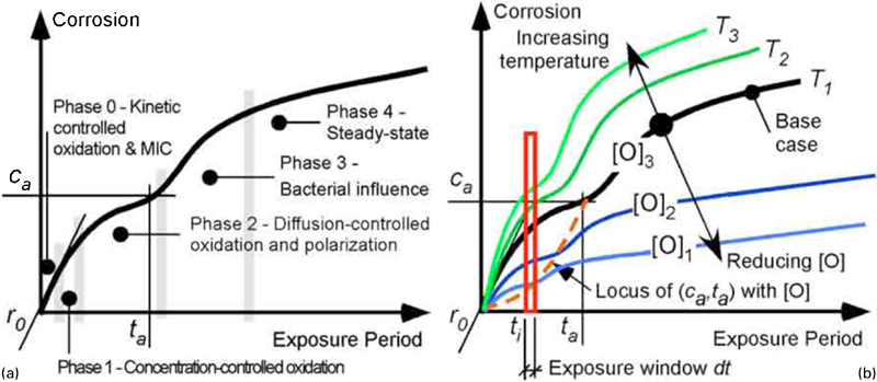
a schematic corrosion loss model showing phases controlling corrosion and model parameters t a, r 0 and c a and b effect of reduction in dissolved oxygen content and effect of increasing water temperature: also shown is exposure window discussed in text
The model is composed of five sequential phases each describing a different dominant corrosion mechanism. These are summarised in Fig. 1a. The principal corrosion rate controlling mechanism in the period 0<t<t a is diffusion of oxygen through the increasing thickness (and hence reducing permeability) of the rust layers. The effect of the availability of oxygen, expressed through the bulk water dissolved oxygen concentration [O], is shown schematically in Fig 1b. More details are available.8 Also shown, schematically, in Fig 1b is the effect of water temperature, which is an important influencing factor for most model parameters.6,8 The terms r 0, t a and c a parameterise the early part (the first mode) of the model, with r 0 denoting the nominal initial corrosion rate in the short period immediately after t = 0, t a is the time point at which there is an up-swing in the corrosion rate (and the commencement of the second mode), and c a denotes the corresponding corrosion loss at that time. The parameters for the later part of the model are not of particular interest for the exposition to follow. To be sure, estimation of these parameters involves a degree of subjectivity but despite this a high degree of consistency of the parameters has been found across many sets of data.6,8
The development of the model included the likelihood that microbiologically influenced corrosion (MIC) plays a role in the corrosion process. As summarised earlier8 this is known to be a factor particularly in phases 0 and 3 and to a lesser extent in phase 4 of the model, at least for seawater corrosion.8 The effect of MIC on freshwater corrosion is much less known but has been seen previously in laboratory studies over exposure periods up to 12 months.9 Whereas in seawater the bacteria most commonly associated with MIC are the sulphate reducing bacteria whose metabolism (and growth and activity) is governed by nutrient (and energy) availability and in particular nitrogen availability, for freshwater the limiting nutrient(s) usually are sulphates, unless there is significant sewage or similar nutrient pollution.10 Calcium carbonate in hard waters is thought to reduce the availability of sulphates,11 depressing the metabolism of bacteria and thus reducing short term corrosion rates. This explains why moderate changes in nutrient levels can cause significant increases in corrosion, inconsistent with changes in the rate of (electro-)chemical corrosion to be expected from direct changes in the chemical composition of the water. The bacteria involved in freshwater corrosion also are different.12,13
Separately from any effect water hardness may have on the availability of nutrients, the calcium and magnesium carbonates primarily responsible for water hardness tend to deposit within the corrosion product layer formed on metals exposed to waters with high concentrations of these carbonates.14 This is the case for seawater (which usually is supersaturated with carbonates) and also for hard freshwaters. The carbonates contribute to the formation of adherent, protective calcareous deposits at cathodic areas, particularly at a higher pH.14,15 The deposits have a relatively high electrical resistance and hence reduce the effective cathodic area, thereby reducing corrosion currents and hence corrosion. Equivalently, the effect can be described as the carbonates tending to reduce the diffusivity of the rusts on the corroded surface thereby reducing the rate of supply of oxygen and hence reducing the corrosion rate. Evidently, this effect is a direct function of water pH, a matter recognised already many years ago. One result is that so called soft waters (those with low levels of dissolved carbonates) can be very corrosive, irrespective of chloride content.3
The parameters for the early part of the model have previously been estimated for mild steel exposed in natural seawaters below 29°C, based on a large number of field observations.6 Trends for these data have been derived and are extrapolated below to consider them in relation to data for corrosion at higher water temperatures.
Warm water corrosion data
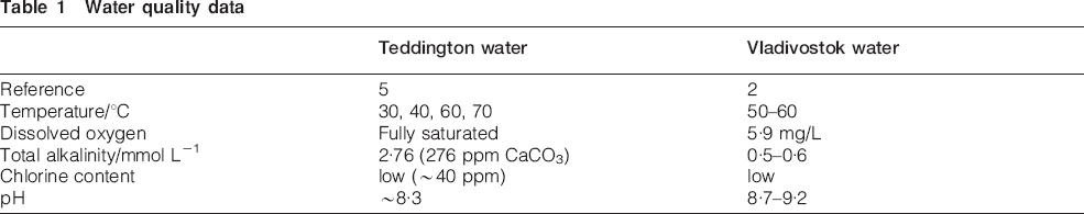
As part of a much wider laboratory study, Mercer and Lumbard5 reported corrosion loss data for mild steel immersed continuously in fully oxygen saturated Teddington tapwater at temperatures in the range 5-95°C. The water was hard, had a low chloride content and pH≈8·3 (Table 1). The specimens were 15 mm diameter circular mild steel coupons, 40 mm long, rotated at 1 Hz. Several tests were conducted with different water temperatures and dissolved oxygen contents but only one set of data (at 70°C) was reported in sufficient detail to construct a curve of mass loss as a function of exposure period (Fig. 2).
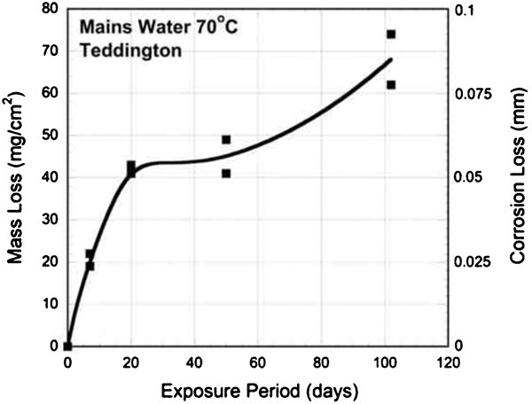
Mass loss data and best fit trend (see text) for corrosion loss as function of exposure period for rotating mild steel coupons exposed in 70°C hard fresh Teddington (UK) water5
Water quality data
In Fig. 2 the best fit smooth trend curve was constructed through the data using the Stineman function, a locally weighted (10% of data) least squares fit.16 The resulting corrosion–loss function trend is seen to be consistent with Fig. 1. From Fig. 2 estimates were made for the parameters t a, r 0 and c a at 70°C.
The data provided by Mercer and Lumbard5 is insufficient information to construct corrosion mass loss curves such as Fig. 2 for other water temperatures in the range 29-70°C. However, they do quote corrosion losses at 49 days exposure for a number of different water temperatures T in the range 0-95°C (Fig. 3) and remarked that the data appeared to show no clear systematic behaviour. These data can, however, be given a rational explanation with the aid of Fig. 1 and using well accepted corrosion theory principles. Consider the exposure window shown in Fig. 1b at t i with dt→0, and also the variation in the corrosion loss curve as the water temperature T increases. The corrosion loss curve moves to the left and in doing so the principal model corrosion phase observed in the window changes from phase 1 to phase 2. From this it can be deduced that c a is sensitive to T in phase 1 but rather insensitive to T in phase 2. Therefore, in Fig. 3 the mass losses for T<25°C refer mainly to phase 1 and those in the range 25°C<T<80°C mainly to phase 2. At higher water temperatures the solubility of oxygen in water reduces quickly and the corresponding mass loss observations cannot be compared with those for lower water temperatures.5 The data shown in Fig. 3 can be converted readily from mass loss per unit area to corrosion loss in the range 30-70°C and in turn interpreted as c a.
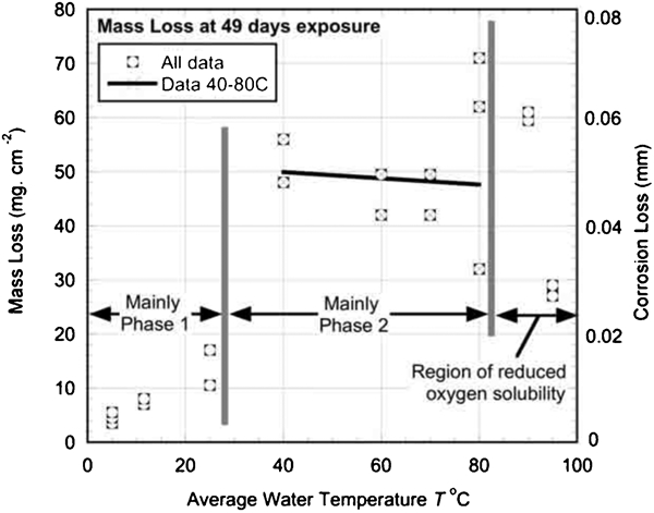
Mass loss as function of water temperature at 49 days exposure reported by Mercer and Lumbard5 showing that lower water temperatures are associated with phase 1 of corrosion loss model (Fig. 1) and waters in range 30-70°C with phase 2: results for higher water temperatures are influenced by reduced oxygen solubility; right axis shows interpreted equivalent corrosion losses that, for phase 2, can be interpreted as c a values
Mercer and Lumbard5 also quote measurements of corrosion potentials E as a function of water temperature T (Fig. 4), stating that the potentials may be interpreted as proportional corrosion rates when corrosion is under cathodic control, as is implicit in the model of Fig. 1 and which is consistent with the Evans diagram.7 As a result, the (logarithm of the) corrosion rate i is proportional to E. This allows the data points for 30<T≤70°C to be calibrated to corrosion rates in mm year−1, using the scale shown at right in Fig. 4.
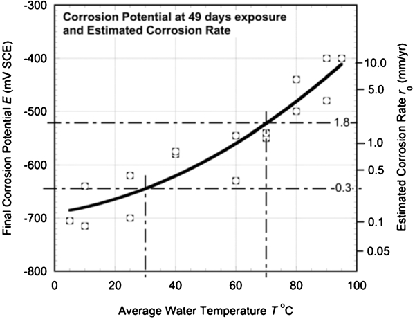
Corrosion potential E as function of water temperature at 49 days exposure based on data reported by Mercer and Lumbard5: trend curve is best fit; equivalent initial corrosion rates r 0 are shown on right axis and calibrated, as shown, at 30 and 70°C
Apart from one value of model parameter t a at 70°C that can be estimated from Fig. 2, there is no information in Mercer and Lumbard5 that can be used to provide estimates of t a at other water temperatures.
Discussion
As noted above, using a large number of field observations, the trends for the model parameters for the early part of the model were earlier estimated for mild steel exposed in natural seawaters below 29°C.6 Figure 5 shows the trend for the parameter c a for seawater exposures and also the results and trends for mild steel exposed to hard freshwaters.3 The two data sets and trends are very similar. The trend for c a can be represented mathematically, as a function of average water temperature T, for each data set, by a shifted exponential function

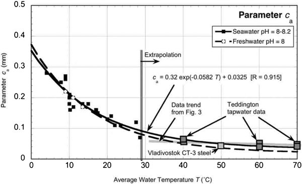
Plot of trends for parameter c a as function of average water temperature T, derived from data in range 0-29°C and extrapolated to 70°C: values of c a derived from Teddington corrosion loss curve at 70°C, taken from Fig. 2, and six estimates at 40, 60 and 70°C taken from Fig. 3, are shown; also shown is c a estimate for Vladivostok data
Figure 6 shows the trends for the initial corrosion rate r 0 extrapolated from the data6 for waters below 29°C. In these cases, data for waters in the pH range 7·5-8·5 are also taken as one data set (Fig. 6). An Arrhenius relationship is used to fit a trend curve to the data. This is appropriate where corrosion is strongly influenced by temperature effects. Figure 6 shows considerable scatter in the freshwater corrosion data below 29°C; nevertheless, the two extrapolated trend curves fall remarkably close together. Figure 6 also shows the estimate of r 0 from Fig. 2, and the estimates for r 0 given in Fig. 4 for parameters derived for the water temperatures used in the Mercer and Lumbard5 experiments. The estimated value of r 0 for the Vladivostok data4 is also shown. It is considerably lower in value than the trends.
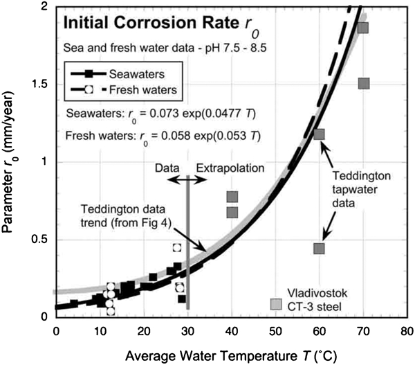
Plot of trends for initial corrosion rate r 0 as function of average water temperature T, derived from data in range 0-29°C and extrapolated to 70°C: value of r 0 derived from Teddington corrosion loss curve at 70°C, taken from Fig. 2, and six estimates at 40, 60 and 70°C taken from Fig. 4, are shown; r 0 estimate for Vladivostok data is also shown
Figures 5 and 6 show that the parameters derived from the interpretation of the Teddington hard water corrosion experiments provide, for c a and r 0 respectively, values that are consistent with the respective trend curves extrapolated from the data below 29°C. In both cases the trends show a smooth transition of the parameter values between cooler waters and those to 70°C. This supports the notion that there are no sudden changes in the corrosion processes.
The trend for t a extrapolated to 70°C is shown in Fig. 7. It differs somewhat from that obtained earlier for the Vladivostok data.4 Previously a difference was observed between the trends for seawater and for freshwater at about the same pH at water temperatures around 25-30°C. Closer examination of the data showed that this difference was due entirely to one value for t a estimated from the corrosion loss curve for field exposure at 27·6°C at Coco Solo, in the Panama Canal Zone.17 The data for this site were re-examined, also for consistency with data for other generally similar exposure sites. As a result the value for t a was lowered so that it is now generally in accord with the other data. Therefore, only one trend line need to be shown in Fig. 7.
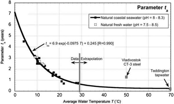
Plot of trend for parameter t a as function of average water temperature T, derived from data in range 0-29°C and extrapolated to 70°C: value of t a derived from Teddington corrosion loss curve at 70°C (Fig. 2) is shown; value of t a estimated for Vladivostok data is shown
Figure 7 also shows the one value of t a that could be estimated from Fig. 2 for Teddington freshwater. As noted, there is no other data5 that can be used for estimation of t a. (This is understandable since that parameter had not yet been proposed at the time the experiments were conducted.) Nevertheless, from Fig. 1 it can be observed that t a is related to r 0, with lower r 0 producing longer values of t a. This indicates that the trend for t a should be inversely proportional to that for r 0. Given the gradual changes in r 0 shown in Fig. 6, a gradual change from the value of t a below 30°C to the value shown at 70°C can be assumed and this is also predicted in the trend line shown. Therefore, while there is only one direct data point for t a (i.e. that at 70°C) for water temperatures above 29°C, the trend shown in Fig. 7 can be considered reasonable and consistent with the (limited) available data.
Overall, the correspondence between the parameter values derived from the Teddington experimental observations and the respective trends may be considered remarkable, given the very considerable extrapolation that is required from the data in the range 0-29°C. However, the values of t a and r 0 estimated earlier from the Vladivostok data4 clearly are at odds with the trends in Figs. 6 and 7. The likely reason for this is that the Vladivostok data2 were obtained under very low velocity conditions. In contrast, the corrosion field observations for waters below 29°C were all for natural freshwater streams and coastal seawaters and these waters all have non-negligible water velocities. Previously it was estimated that for coastal seawaters the average water velocity is in the range 0·05-0·15 m s−1, although this may vary considerably, both daily and seasonally, and may be much higher for short periods.18 Also, the Teddington results were obtained for specimens rotating at a constant angular velocity and for the 15 mm diameter specimens used this corresponds to a constant tangential velocity of ∼0·05 m s−1, which is comparable with the typical water velocities in natural exposures.
Water velocity has most effect while there is little or no corrosion product on the surface of the steel.18 High water velocity reduces the thickness of the oxygen concentration gradient immediately beside the metal surface when it is first exposed.19 Conversely, in quiescent waters the thickness of the oxygen concentration gradient is reduced at a a lower rate and as a result the rate of early corrosion will be lower, consistent with the lower initial corrosion rate r 0 for Vladivostok in Fig. 6. However, water velocity has much less effect on c a18 which is consistent with the Vladivostok data showing the parameter c a close to the trend line in Fig. 5. Finally, for t a it is observed first that as the water velocity reduces r 0 also reduces and thus the progression from phase 1 to phase 2 and from phase 2 to phase 3 is delayed (Fig. 1). This means that the time point t a at which the change from phase 2 to phase 3 occurs, also will be delayed, consistent with the high value of the Vladivostok data point relative to the trend line in Fig. 7.
Conclusions
A new set of interpretations is given for data reported by Mercer and Lumbard in 1995 for corrosion of mild steel in hard fresh waters in the range 30-70°C.
This new interpretation is shown to provide estimates for the parameters of the bimodal corrosion model that are consistent with the trends extrapolated from data in waters at lower temperatures.
Model parameters estimated for data obtained under very low water velocity conditions show general consistency with the extrapolated trends provided allowance is made for the known effect of water velocity on longer term corrosion.
The present analysis extends the range of applicability of the bimodal model to higher water temperatures for fresh hard water and, by implication, also for seawater.
Footnotes
Acknowledgements
R. E. Melchers acknowledges the support of the Australian Research Council.