High sensitivity electrical resistance sensors for indoor corrosion monitoring

Abstract

It is essential that corrosion monitoring of indoor atmospheres be highly sensitive, especially when corrosion rates corresponding to the lowest standard corrosivity categories are supposed to be identified within one or a few days. The electrical resistance (ER) technique in combination with high sensitivity ER sensors enabled detection of corrosion loss on an atomic scale. The magnetron sputtering method was used to produce sensors equipped with 50 to 800 nm metallic track. The set of developed sensors represent a wide range of materials, e.g. copper, silver, iron, lead and bronze. Laboratory experiments have proven that copper and silver sensors respond to changes in relative humidity and temperature within minutes. Bronze and copper sensors are able to detect changes in concentrations of volatile organic acids, which are common pollutants of indoor atmospheres in museums.

Keywords

Electrical resistance Corrosion monitoring Thin film sensor Magnetron sputtering Corrosivity classification

Introduction

The electrical resistance (ER) technique is one of the methods used for corrosion monitoring. It records corrosion loss in metal thickness in time, and the slope of the curve corresponds to the corrosion rate. Deviations from the curve slope indicate changes in corrosion conditions, whose information is effectively used to identify the causes of corrosion aggressiveness elevation and to verify the effectiveness of the respective corrosion measure, i.e. it acts as an early warning. The method is especially recommendable for the detection of the onset of corrosion.1 Another advantage of the ER technique is that in contrast to electrochemical methods the presence of an electrolyte layer on the metal surface is not inevitable. In that sense, there are no problems with the method being used is atmospheric conditions even at a low relative humidity (RH) of atmosphere.1 Moreover, it is used for corrosion monitoring of high temperature corrosion, erosion corrosion or in non-conductive environments. Despite other methods2 ^– 9 used for monitoring atmospheric corrosion, the resistometric method provides information directly about the metal corrosion loss.

The sensors for corrosion rate testing using the resistometric method must comply with certain sensitivity and service life requirements. High sensitivity is achieved by a small thickness of the sensor metallic track. Compared to a less sensitive sensor, the disadvantage of a thin metallic track is its shorter service life. The appropriate thickness of the metallic track thus depends on what sensitivity and service life the user needs for the anticipated corrosion conditions. As to indoor conditions with the corrosivity ranging from IC1 to IC5,10 metallic track thicknesses tend to be opted in the order of tens and hundreds of nanometres. For outdoor conditions with corrosivity category C2,11 it is recommendable to use sensors with the metallic track ranging within the orders of units and hundreds of micrometres so as to ensure their functioning for at least 1 year.

Monitoring of the corrosion rate corresponding to the lowest corrosivity categories of indoor atmosphere corrosion aggressiveness is inevitable to make sure that, for instance, sensitive electronic equipment is protected and that metallic artefacts are treated right and safely when exhibited, transported or stored in depositories.9 The atmosphere corrosivity category is determined on the grounds of the corrosion rate of steel, zinc, copper and silver. Corrosion rates ranging within the order of hundreds of mg m⁻² a⁻¹ correspond to the second lowest corrosivity category IC2. Expressed by the loss in metal thickness in time, corrosion rates in IC2 atmosphere correspond to the order of tens of nm a⁻¹. Hence, should the corrosion monitoring system be able to provide an early warning, i.e. within 24 h, that corrosivity increased by one category, the corrosion sensor must be able to detect the change on the metallic track thickness within the order of tenths of nanometres. Such sensitivity was approached by Cai and Lyon12 with their zinc and steel based resistometric sensors.

Standards for corrosivity classification introduce four metals only, although other metals may differ in their response to a great extent. Whereas zinc and steel or iron are very sensitive to sulphur dioxide, silver in contrast to iron is highly sensitive to sulphane.13 Compared to all the other common metals, lead is the most sensitive to organic acids.13,14 Especially for its specific corrosion behaviour and its frequent presence among metallic artefacts, lead would deserve a separate and standardised atmosphere corrosivity assessment.

The corrosivity classification has a relatively universal application. As the ISO 11844 standard or the Sacchi and Muller classification15 not only describes corrosivity category determination on the basis of corrosion rate but also enables estimating the corrosivity category according to the conditions (type of indoor atmospheric environment, temperature, RH, etc.), the corrosivity categories can be used to describe the quality of atmosphere from the perspective of materials other than metals.16 Air reactivity monitoring is a method of evaluating the quality of makeup and recirculation air characterising the museum or archive environment and evaluating the effectiveness of chemical filters.17

This paper presents a set of new corrosion sensors that can be used for high sensitivity corrosion monitoring, and extends the portfolio of high sensitivity sensors by materials that are common in historical artefacts, but whose corrosion rates are not registered in corrosivity classification standards. The sensors’ design has been innovated so as to avoid inaccuracies in thickness loss testing caused by non-uniform corrosion on the interface of the sensing and reference parts of the sensor.

Experimental

Electrical resistance technique

The traditional ER technique is based on identification of the change in electric resistance of a thin layer of metal in time. The thinner the layer of metal as a result of corrosion, the higher the electric resistance of the metallic track. Moreover, the electric resistance of metals depends on temperature because of its positive temperature coefficient. Therefore, a compensation of the temperature dependent drift of ER is a must. This compensation is realised by a division of sensor into corroding and non-corroding parts by measurement of both resistances and calculation of their ratio. The corroding part of the sensor is called a coupon or a sensing part, and the non-corroding part acts as a reference part. The reference part of the sensor has a similar shape to that of the sensing part but is covered with a protective coat to be separated from the corrosion environment. The traditional relation for calculating corrosion loss based on the ratio of real time resistances, initial resistances and initial thickness of the metallic track has the following form18 (1) where h ₀ is the initial thickness of the sensor's metallic track, Δh is the mean thickness loss, R _ref is the ER of the reference part, R _sens is the ER of the sensing part, R _ref,0 is the initial ER of the reference part and R _sens,0 is the initial ER of the sensing part.

This relation anticipates the same initial thickness for both sensing and reference parts. However, this assumption is not always lived up to, which is demonstrated by the fact that the initial resistances of the sensing and reference parts are never ideally identical. The testing itself in the corrosion environment is often preceded by restoration of the sensing part surface by smooth grinding or pickling, which abandons the assumption of identical thicknesses. We have adjusted the relation so that the assumption of a known initial thickness is always met. The thickness of the reference part, which does not essentially change throughout the sensor's service life, acts as the initial thickness in relation (2). Should the sensor be used repeatedly, the user must remember the initial resistance of the sensing part that has not been affected by corrosion when using relation (1). 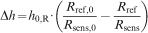The new relation (2) eliminates this limitation (2) where h _0,R is the initial thickness of the reference part.

Precision of the method depends on the accuracy with which electric resistances are determined. The most used method is the four-wire resistance measurement. The ratio of electric resistances of reference and sensing parts can be measured by an ac bridge network.1 The loss of metal thickness or the corrosion rate can be expressed as a ratio of resistances of the corroding track at the start of exposure and at a given time.12,19 Figure 1 shows the traditional shape of atmospheric corrosion sensors,18,20 where the testing current passes between two terminal circuit contacts with the voltage that let the current pass through the metallic track being measured between two other spots on the sensing and reference parts.

Figure 1

Traditional concept of atmospheric corrosion sensor

Sensor's design

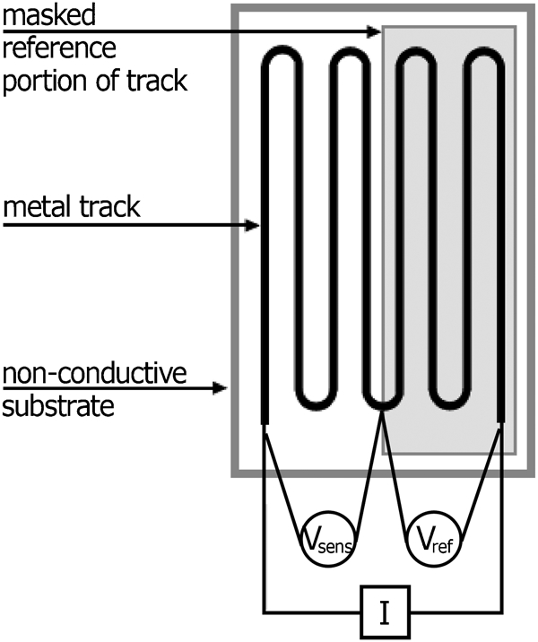
The coat protecting the reference part from corrosion is usually applied so as to have the edge pass through the symmetry axis of both parts of the sensor (Fig. 1). However, the organic coat and metal interface tends to be a weak point in terms of corrosion protection. The protective coat may be undercorroded, and the metallic track on the sensing and reference part interface may be intensively attacked. The original thing about the structure of sensors designed and used by us is that the sensor's sensing and reference parts are connected by an H shaped bridge, and the protective coat borderline passes approximately in the middle of the bridge (Fig. 2). Despite the traditional design (Fig. 1), the borderline of the protective coat is a part neither of the sensing nor the reference part as the bridge serves only as a conductor for passage of testing current, and the voltage scanning points are placed in a safe distance from the coat edge.

Figure 2

New concept of atmospheric corrosion sensor

Manufacturing of sensor

The indoor sensors were produced by means of magnetron sputtering, a technology that is referred in some recent studies.19,21 Manufacturing comprises of the deposition of contacts, a thin film deposition by vacuum technology and vapour mask structuring. A fine grained Al₂O₃ alumina was used as substrate material. Copper, silver, bronze (CuSn8), lead and iron sensors were prepared. Examples of sensors without the reference part protection are shown in Fig. 3.

Figure 3

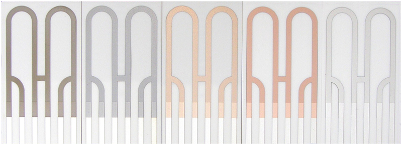
Examples of high sensitivity atmospheric corrosion sensors: Pb–400 nm (left), Fe–800 nm, CuSn8-400 nm, Cu–50 nm, Ag–50 nm (right)

Loggers

AirCorr I and AirCorr I Plus loggers (NKE electronics) were used to measure and record the corrosion losses of high sensitivity corrosion sensors. They are autonomous battery driven loggers equipped with a built in connector providing connection to corrosion sensors. The AirCorr I version employs one corrosion sensor within a given period of time, while the AirCorr I Plus version works with two sensors, recording concurrently the RH and temperature. Results are recorded by WinAirCorr software (NKE electronics).

Results and discussion

Sensitivity and reproducibility tests of corrosion sensors

A great advantage of laboratory tests is the possibility to control exposure conditions with a relative accuracy. Corrosion sensors were thus exposed to various regimes under changing conditions, response of corrosion sensors to the changed conditions was monitored and reproducibility of the response was assessed. Temperature and relative atmospheric humidity were the only features changed during the first experiment, without any corrosion stimulator being added to the corrosion atmosphere. The curves of RH and temperature in time are described in Fig. 4.

Figure 4

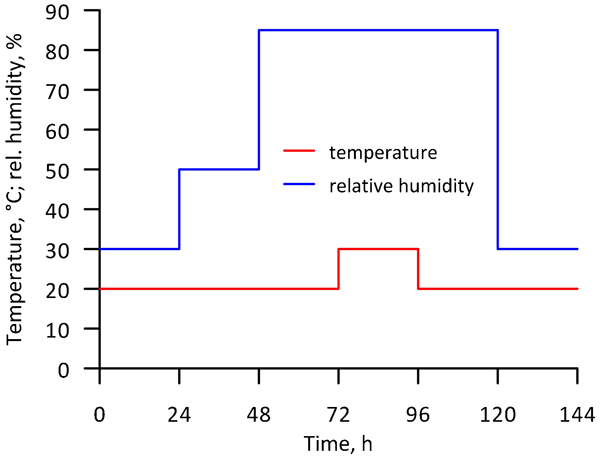
Temperature and relative humidity variations during laboratory corrosion testing

Figure 5 records corrosion loss (reduction of metallic track thickness in the sensing part of the sensor) in time for four concurrently exposed copper sensors. The initial thickness of the sensor metallic track was 500 nm. The design of the sensor was meant to ensure that the sensor's service life was at least 2 years under the conditions of a medium corrosivity indoor atmosphere that corresponds to the corrosivity category of IC3 according to the ISO 11844-1 standard. The overall view (Fig. 5) shows that the sensors react to the increase in RH from 50 to 85% at 20°C. The increase of temperature by 10°C immediately accelerates the corrosion rate. The corrosion loss versus time curve during one 24 h period of time has a parabolic shape, which is typical for copper corrosion under atmospheric conditions.13 The total corrosion losses assessed after six daily cycles were 6·6, 5·2, 5·8 and 6·1 nm. The deviation of extreme values from the mean value does not exceed 12%. Such reproducibility can be considered excellent in the area of corrosion monitoring. Another question is whether the recorded corrosion loss corresponds to the corrosion loss of the metal bulk, i.e. what is the accuracy of corrosion rate determination by copper resistometric sensors. For that purpose, corrosion copper coupons were exposed with the sensors, and their corrosion was coulometrically evaluated after exposure. A negligible layer of corrosion products was galvanostatically reduced, and the amount of copper that converted in an oxidised form during the corrosion test was calculated from the charge necessary for reduction. This amount recalculated to the loss of thickness of three coupons exposed in parallel corresponded to 5·2, 6·2 and 6·3 nm. The coulometrically specified average loss of thickness of cooper is equal to the mean value of the loss of thickness identified by the resistometric sensor.

Figure 5

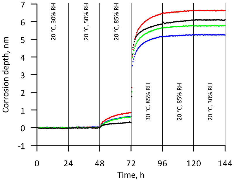
Corrosion depth record of four parallel Cu–500 nm sensors exposed to varying temperature and RH

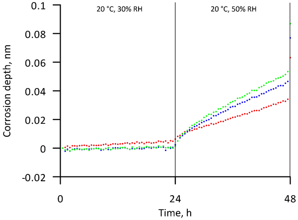
Copper sensors react to the increase in RH from 50 to 85% almost immediately. The time to respond was shorter than the selected sampling period of 15 minutes. The sensor with a 500 nm metallic track is not able to detect corrosion at RH lower than 50%. In spite of that, the sensor's sensitivity is sufficient for detecting processes on an atomic level, where corrosion converts one layer of metal atoms, i.e. on the level of tenths of nanometres. A copper sensor with a 50 nm metallic track provides even higher sensitivity (Fig. 6).

Figure 6

Corrosion depth record of three parallel Cu–50 nm sensors exposed to varying temperature

For a cut of the graph of the corrosion loss of three copper sensors exposed in parallel with a metallic track thickness of 50 nm, see Fig. 6. Reproducibly recorded thickness losses on the level of hundredths or even thousandths of nanometres may be merely considered a conversion of a specific amount of metal atoms on the cross-section of the metallic track in an oxidised form, i.e. corrosion products rather than a uniform loss of metal over the entire exposed surface. Such high sensitivity is essential for corrosion monitoring that must be able to detect a change of corrosivity category from IC1 (very low corrosivity) to IC2 (low corrosivity) as defined by the ISO 11844-1 standard within 1 day, yet ensure at least 1 year service life for corrosivity IC2.

From a practical point of view, silver sensors with a 50 nm metallic track show the same sensitivity as Cu–50 nm copper sensors. The corrosion loss is again recorded reproducibly with accuracy on the level of hundredths and thousandths of nanometres (Fig. 7). Moreover, the change of RH from 30 to 50% did not cause any change of the slope of the corrosion loss versus time curve, which confirms a well known fact that silver sulphide developing in indoor atmospheres due to the presence of traces of sulphane at low RH is formed as a result of direct chemical reaction with silver, and the slope is thus not much dependent on the presence of water.22

Figure 7

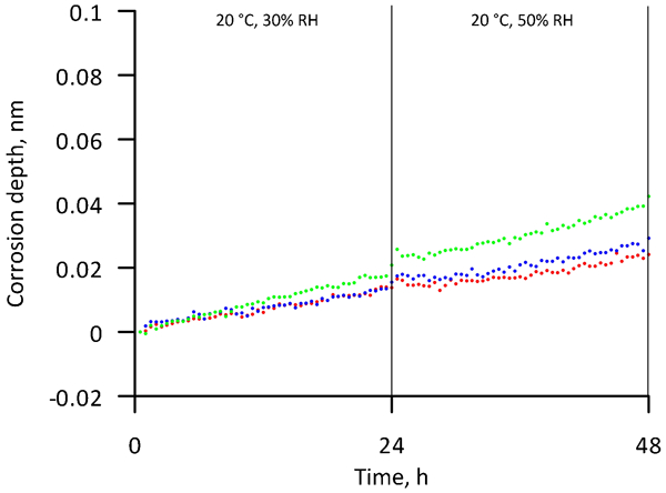
Corrosion depth record of three parallel Ag–50 nm sensors exposed to varying temperature

The response of lead and iron sensors was tested the same way. As shown in the graph (Fig. 8), reproducibility of the measurements of the loss of thickness of these materials is remarkably lower than in the case of sensors made from silver and copper. It is probably given by more frequent localised attacks in the starting phases of corrosion of these metals, namely, iron. However, it is obvious that corrosion losses of iron and lead are higher by an order under the same conditions than those of silver and copper, with lead being specifically sensitive to volatile organic substances in the atmosphere. Therefore, it may be advisable to use sensors made from lead and iron for corrosion monitoring of these metals instead of deriving their corrosivity from the responses of silver and copper.

Figure 8

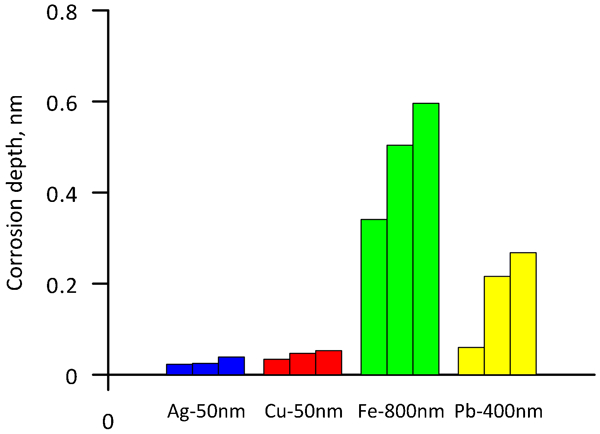
Total corrosion depth of three parallel sensors after test cycle at varying temperature and relative humidity

Laboratory tests in air contaminated with organic acids

A chamber allowing for corrosion measurements in air with low and well controlled concentrations of gaseous pollutants was designed. A setup consisting of an air dehumidifier, air filter, gas generator, humidifier, exposure chamber and exhaust air treatment unit has been built. A polluted air generator produces the target pollutant level. This gas generator includes an oven with temperature precisely controlled between 30 and 100°C (±0·1°C) and a mass flow controller. It is possible to reach any concentration to ∼1500 ppb of acetic acid and to ∼3000 ppb of formic acid in the outlet air.

A measurement performed in humid air at an RH range from 15 to 80% containing acetic acid at concentrations from 0 to 870 ppb on a bronze thin film sensor with a thickness of 500 nm (CuSn8-500 nm) is given in Fig. 9. The experiment was carried out at 20°C in the chamber described above.

Figure 9

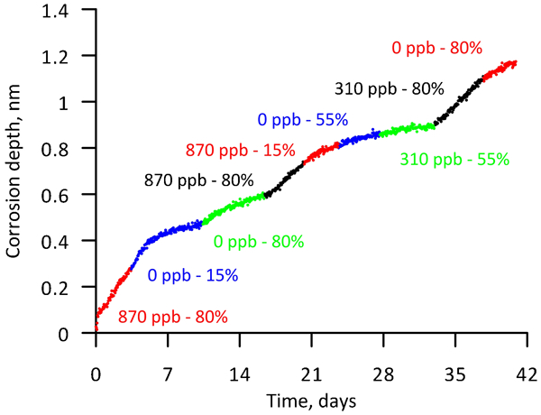
Corrosion depth measured in air containing acetic acid using CuSn8-500 nm sensor: numbers give concentration of acetic acid and relative humidity

It is obvious that the corrosion rate of bronze increased with both RH and acetic acid concentration. The corrosion depth started to increase rapidly after the introduction of the pollutant into the air, which shows the rapid response of the sensor. On the contrary, it took several days until the corrosion rate started to decrease after a decrease in pollutant concentration. This was observed even under conditions where the RH was also reduced to low levels, see e.g. the transition 870 ppb–80% RH to 0 ppb–15% RH in Fig. 9. Since the air in the chamber is exchanged within ∼15 min, this indicates that a film of the adsorbed pollutant was present on the metal surface long after the pollutant was removed from the air.

A simple model for the effect of the acetic acid air concentration and RH on the corrosion rate of bronze was proposed. The corrosion rate r _corr can be expressed as (3) where c _AA is the concentration of acetic acid in ppb, RH is the relative humidity in % and A and B are constants.

A similar experiment was carried out in air containing formic acid at concentrations from 0 to 1590 ppb and at RH from 15 to 80%. However, the air corrosivity was increased systematically in this experiment in order to establish a threshold level of the formic acid concentration, which leads to an unacceptable corrosion rate of the materials tested. Cu–500 nm, Pb–800 nm and Fe–800 nm sensors were tested in three replicates.

The corrosion depth record for a Cu–500 nm sensor is plotted in Fig. 10. The experiment started in clean air at 15% RH. The corrosion rate was below the detection limit until the RH was increased to 70%. It stabilised after ∼4 days at 4-5 nm a⁻¹ and did not change although the RH was further increased to 80%. No dramatic effect of formic acid on copper corrosion was observed at concentrations from 10 to 220 ppb. When the formic acid concentration increased to 460 ppb, the corrosion rate changed to ∼20 nm a⁻¹. It stayed at this level at 1000 ppb as well.

Figure 10

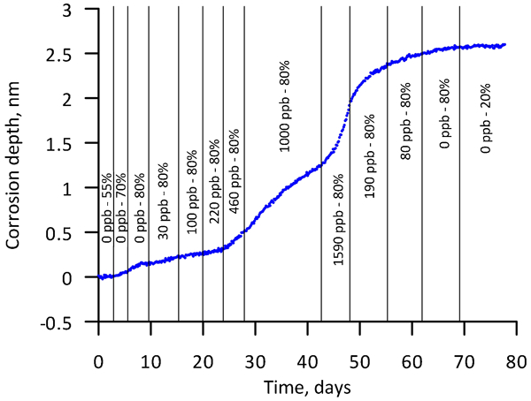
Corrosion depth measured in air containing formic acid using Cu–500 nm sensor: numbers give concentration of formic acid and relative humidity

A further increase in corrosion rate to ∼50 nm a⁻¹ was noted at the maximal formic acid concentration of 1590 ppb. When the concentration was dropped to 190, 80 and 0 ppb, the corrosion rate decreased gradually to low values.

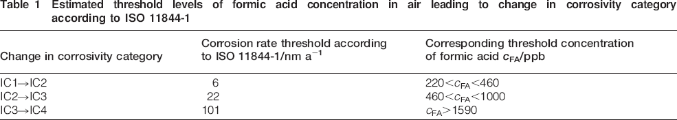
Based on the conducted experiments, the threshold levels of formic acid in air at 80% RH and at 20°C for corrosivity categories defined by the ISO 11844-1 standard can be estimated (see Table 1). Such a formic acid concentration has been reported in museums, churches and other cultural heritage premises by several authors.23 ^– 26

Table 1

Estimated threshold levels of formic acid concentration in air leading to change in corrosivity category according to ISO 11844-1

Change in corrosivity category	Corrosion rate threshold according to ISO 11844-1/nm a⁻¹	Corresponding threshold concentration of formic acid c _FA/ppb
IC1→IC2	6	220<c _FA<460
IC2→IC3	22	460<c _FA<1000
IC3→IC4	101	c _FA>1590

Conclusions

Magnetron sputtering enables the production of a wide range of metals with a precisely controlled deposition of the metal layer thickness that determines the sensitivity of the resistometric sensor for measuring corrosion loss.

The sensitivity of sensors on an atomic level was identified under the conditions of changing temperature and RH when corrosion changes one layer of metal atoms, i.e. on the level of tenths of nanometres. Reproducibly recorded thickness losses of very sensitive sensors on the level of hundredths of nanometres may be merely considered a conversion of a specific amount of metal atoms on the cross-section of the metallic track into corrosion products rather than a uniform loss of metal over the entire exposed surface. Such high sensitivity is essential for corrosion monitoring that must be able to detect a change of a corrosivity category from IC1 (very low corrosivity) to IC2 (low corrosivity) as defined by the ISO 11844-1 standard within 1 day, yet ensure at least 1 year service life for corrosivity IC2.

The recorded corrosion loss versus time curves confirm the well known facts about the corrosion processes kinetics in atmosphere and the different sensitivities of various metals to different pollutants. High sensitivity resistometric sensors may thus be used for studying the kinetics of corrosion processes.

The reproducibility of measurements of corrosion losses of copper and silver is high compared to the reproducibility identified for lead and iron sensors.

Footnotes

Acknowledgements

The authors gratefully acknowledge the financial support by the European Commission under the Seventh Framework Programme (contract no. 226539) and by the Czech Ministry of Education under special purpose support to college research programmes (resolution no. 21/2011).

References

McKenzie

Vassie

: Br. Corros. J. 1985 20 117–124.

Fraigi

Gwirc

Lupi

: Sens. Actuators B 1994 19B 558–561.

Pacheco

AMG

Ferreira

MGS

: Corros. Sci. 1994 36 797–813.

Jung

Kim

Song

Lee

Kho

: Corros. Sci. Technol. 2002 31 383–387.

Noda

Takaya

Hideki

Hiroyuki

Toshiaki

: Proc. 15th Int. Corros. Cong. on ‘Frontiers in corrosion science and technology’ Granada, Spain September 2002 International Corrosion Council and Spanish Council for Scientific Research 595/1–595/7.

Saitou

Oshikawa

Itomura

Tsuzikawa

: J. Chem. Phys. 1999 110 (24) 12122–12124.

Shinohara

Motoda

Oshikawa

: Mater. Sci. Forum 2005 475-479 61–64.

Shitanda

Irisako

Itagaki

: Sens. Actuators B 2011 160B 1606–1609.

Zakipour

Leygraf

Portnoff

: J. Electrochem. Soc. 1986 133 873–876.

10.

‘Corrosion of metals and alloys – classification of low corrosivity of indoor atmospheres – Part 1: determination and estimation of indoor corrosivity’

ISO 11844-1

International Organization of Standardization

Genève, Switzerland

2006 5.

11.

‘Corrosion of metals and alloys – corrosivity of atmospheres – classification, determination and estimation’

ISO 9223

International Organization of Standardization

Genève, Switzerland

2002 6.

12.

Cai

Lyon

: Corros. Sci. 2005 47 2956–2973.

13.

Leygraf

Graedel

: ‘Atmosfpheric corrosion’38103; 2000

New York

Wiley Interscience.

14.

Odlyha

Theodorakopoulos

Thickett

Ryhl-Svendsen

Slater

Campana

: ‘Museum microclimates: contribution to the Copenhagen conference’ Copenhagen, Denmark, November 2007, The National Museum of Denmark73–79.

15.

Sacchi

Muller

: American Society of Heating, Refrigerating & Air-Conditioning Engineers 2005 7.

16.

Havermans

: ‘Indoor air quality in museums and archives’ Chalon-sur-Saône, France, April</month> 2010 SARL Germolles37.

17.

Purafil : ‘The OnGuard 3000 for museum and archive applications’ available at: http://www.purafil.com/products/monitoring/onguard3000_museum.aspx (viewed 2012 July 17).

18.

Sjögren

Le Bozec

: ‘On-line corrosion monitoring of indoor atmospheres’, Proc. Eurocorr 2004, Nice, France September 2004, European Federation of Corrosion.

19.

Kim

Jung

Song

Lee

: Sens. Actuators B 2007 120B 368–377.

20.

RCS : ‘Environmental monitoring’ available at: http://www.cosasco.com/environmental-monitoring.html (viewed 2012 July 17).

21.

Kim

Jeon

Kho

Kang

: Corrosion 2001 57 815–828.

22.

Volpe

Peterson

: Corros. Sci. 1989 29 (10) 1179–1196.

23.

Gibson

Cooksey

Littlejohn

Tennent

: Anal. Chim. Acta 1997 341 (1) 1–10.

24.

Gibson

Watt

: Corros. Sci. 2010 52 (1) 172–178.

25.

Chiavari

Martini

Prandstraller

Niklasson

Johansson

Svensson

Åslund

Bergsten

: Corros. Sci. 2008 50 (9) 2444–2455.

26.

Ryhl-Svendsen

Glastrup

: Atmos. Environ. 2002 36 (24) 3909–3916.