
Abstract
Cast iron piers of a disused 90 year old multispan railway bridge located close to the Pacific Ocean were extensively sampled for remaining wall thickness to determine corrosion loss and pit depth. From this, a corrosion loss model for the full 90 years was developed. In addition, the statistics for uncertainty in corrosion loss were obtained. Corrosion varied with elevation relative to mean water level and was negligible in the atmospheric zone, about 2-3 mm in the immersion zone and 5-6 mm in the splash and lower tidal zones. This variation is consistent with accelerated low water corrosion. It indicates that water pollution occurred sometime during the life of the bridge. Maximum pit depths were determined and analysed using extreme value statistics. The corrosion model for such long term exposure and the related statistical results are unique and important for assessment of remaining life of the many other cast iron structures still in existence in many parts of the world.
Introduction
Grey cast iron was used extensively in the 1880-1920s for the piers of major railway and roadway bridges. Many of these remain in-service in many parts of the world, some in aggressive marine exposure locations. Surprisingly little has been published about their long term corrosion resistance although it is known, anecdotally, to be generally favourable. 1 For marine exposure conditions, some results are available from the 16 year exposure studies in the Panama Canal Zone (PCZ).2,3 Recently, it was shown that grey (and other) cast irons typically display a bimodal corrosion loss–exposure time characteristic, 4 first proposed for the corrosion of steels exposed to natural exposure conditions including marine immersion, tidal and coastal environments. There appears to be only limited information about the longer term pitting behaviour of cast iron2,3 or about statistical variability in corrosion loss and pit depth. 1 The present paper contributes to all these aspects.
Grey cast iron has a typical grey appearance when fractured, largely the result of its high carbon content, often in the range of 2.5-4 mass-%. One of the remarkable features about the corrosion of cast iron is that the (ferrous) iron content of the surface layers is leached out during the corrosion process, leaving behind a graphite matrix. This graphite matrix is typical of the metallurgical structure of cast irons. 5 After the iron is corroded away, the outside matrix layer becomes filled with rust products. This layer usually is termed (erroneously) the ‘graphitised layer’. 1 It has the same carbon crystalline lattice structure as in the original cast iron; hence, the original thickness of the material remains constant. It also has some low level of strength such that the original surface of the object tends to remain discernable (and is sometimes mistaken for the uncorroded object). For corrosion studies, the major advantage is that the depth of the graphitised zone provides an indication of the corrosion of the cast iron, and its external surface provides a useful reference for measuring the amount of iron lost through corrosion.
The major practical limitation of cast iron is its poor tensile strength. For this reason, it largely has been phased out as a significant structural engineering material. However, since bridge piers largely act in compression, they often are satisfactory for continued service, provided the extent of any corrosion damage is sufficiently low and is likely to remain so for the remainder of the proposed service life. This means that assessment must be possible of the current condition of piers, and the likely rate of future corrosion must be predictable with sufficient accuracy. Corrosion loss models and models for maximum pit depth as functions of exposure time and environmental and other conditions can be of assistance in such prediction.
The present paper is concerned with developing such models, using data obtained from cast iron bridge piers that had been in operation for some 90 years in a marine exposure environment. It also is concerned with obtaining statistical information about the variability in corrosion loss and about the depth of corrosion pitting and their variation with elevation relative to the mean (tidal) water level. The next section describes the measurements that were made of the corrosion losses and pit depths on samples obtained from the piers during the demolition of a disused railway bridge. This is followed by an interpretation of the data relative to results reported earlier for corrosion of cast iron for up to 16 years. In addition, the variability of the corrosion losses at various elevations on the bridge piers is considered and interpreted using trends for corrosion losses for steel extending through the atmospheric, tidal and immersion zones. Further, an extreme value analysis is given of the variability of maximum pit depth as a function of elevation.
Experimental investigations
The bridge available for the present study was located at St Lawrence, a very small township in the Queensland Rail country network. The bridge was constructed in 1920. It was located ∼160 km south of Mackay, ∼6 km from the Pacific Ocean coast and ∼1 km from the major part of the estuary forming the mouth of St Lawrence Creek (Fig. 1).
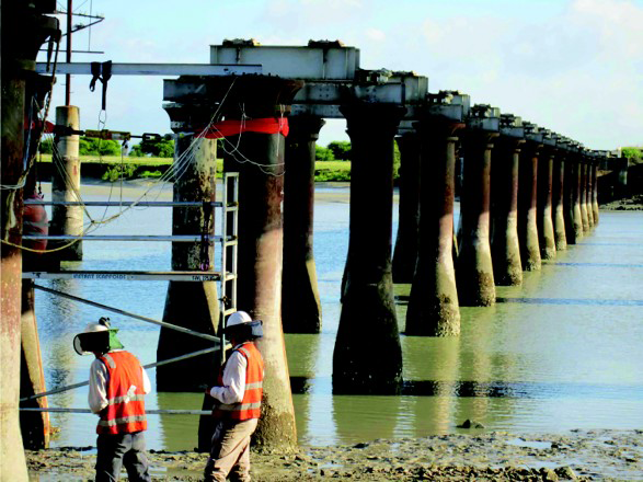
St Lawrence Creek rail bridge immediately before demolition of piers in February 2010 (photo © R. Emslie)
During demolition, 34 coupons, each between 300 × 300 to 400 × 400 mm were sawn from selected piers of the bridge. Figure 2 shows a schematic view of the locations of piers from which the coupons were cut as well as the profile of the creek riverbed relative to the tops of the cones of the piers. The average high, mean and low tide levels also are shown. Two of the piers were sectioned perpendicular to their longitudinal axes to yield four rings, two in the immersion zone and two (smaller diameter) in the atmospheric exposure zone. The samples were all labelled, wrapped in polythene sheet and sealed and forwarded to the University of Newcastle. There, they were stored under cover until ready for examination.
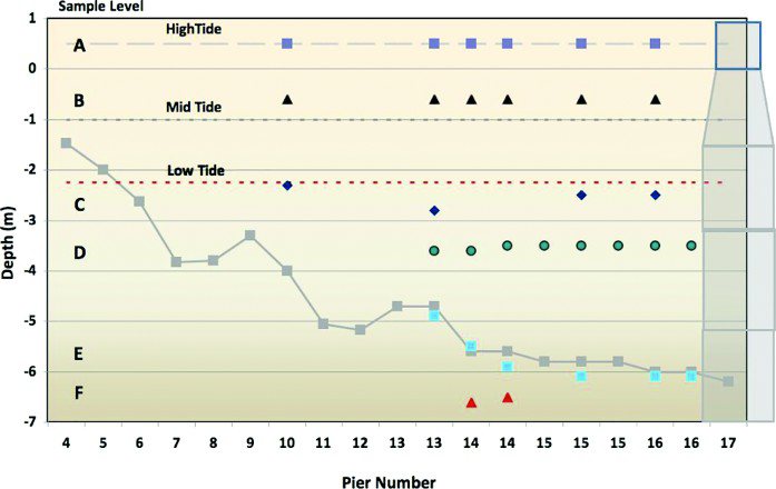
Locations of piers, creek bed and levels (A–F) at which coupons were taken relative to top of pier cone (© R. Emslie)
Each coupon was carefully unwrapped, and any excessive adherent material (Fig. 3) was removed where necessary (in some cases first requiring a jack hammer to remove the more adherent material), taking much care to leave the ‘graphitised’ layer intact. In most cases, only gentle prodding was required to remove the excess material. Eight holes we then carefully hand drilled through the graphitised layer according to the pattern shown in Fig. 4, using a 5 mm diameter drill bit. The remainder of the hole was then drilled out using a specially modified square ended 5 mm diameter drill bit.
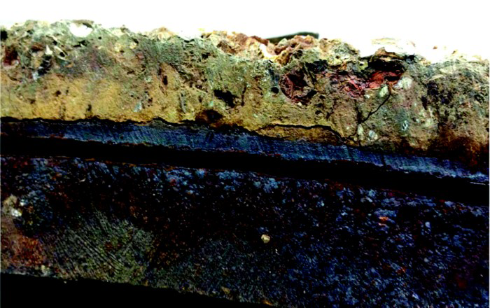
Edge of coupon with adherent material over graphitised layer that already has separated from cast iron under (© C. Herron)
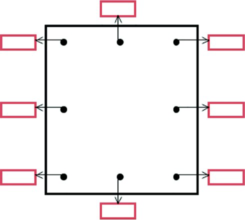
Coupon drill pattern
A specially modified depth gauge was used to measure the depth of the graphitised layer and hence the depth of corrosion relative to the original (but now ‘graphitised’) external surface. All measurements were repeated at each location, and the average was recorded. In addition, observations of the presence of any localised corrosion or pitting were made of all edges of the coupons, where necessary after cleaning of the cut surface with a 100 mm diameter angle grinder and a buffing disc. Where removal of the graphitised layer was required, the coupon was allowed to dry in the open air. This often led to the graphitised layer simply separating from the sound metal underneath. Only in some cases was some small degree of force required for removal.
Two randomly selected samples were analysed for composition. In addition, samples were taken of what appeared to be a calcareous material just below low tide level on one of the piers but well above the current riverbed level and compared with superficially similar material found on samples taken at the riverbed. X-ray diffraction analysis showed the materials to be similar, thereby indicating that the riverbed had changed between original construction and the time of demolition.
The water quality at the site was not measured at the time of demolition as it appeared to be of no interest at that time. The location of the site relatively close to the coastal waters of the Pacific Ocean, the lack of industry in the catchment, the low population in the region and at St Lawrence (population ∼200) and the high tidal flows at the site suggested that water pollution at the site would be insignificant and that the water composition would be similar to natural coastal sea water. As will be shown, the corrosion evidence suggested that this was not the case.
Experimental observations
Composition of cast iron
The average composition of the cast iron samples analysed is shown in Table 1. It is similar to that typical for cast iron at the time of the construction of the bridge. 5
Composition of cast iron recovered from St Lawrence bridge piers (typical, mass-%)

Corrosion losses and maximum depths of pitting
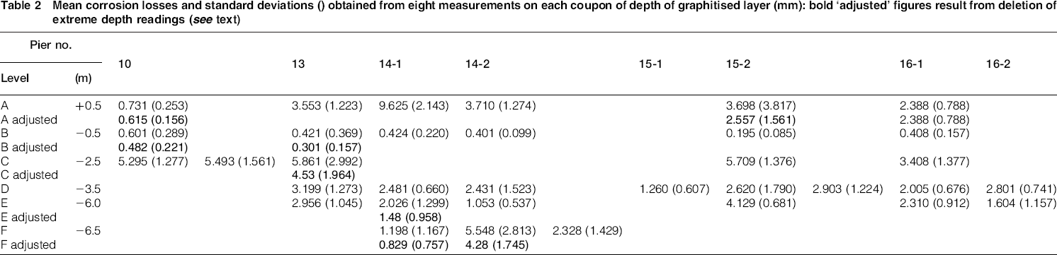
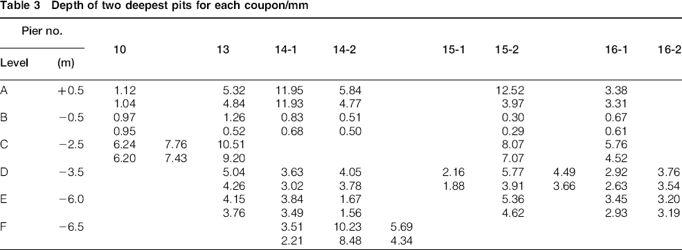
The average of the corrosion losses for each coupon and the associated standard deviations are shown in Table 2 for each pier and location examined. These values were obtained using all eight depth measurements at locations marked on the template (Fig. 4). In some cases, there were large variations in the depth readings, as illustrated in Fig. 5 for coupon 15-2A. The deepest reading, 12.52 mm, is much greater than all the others. It was noted during the measurement procedure that this corresponded closely with localised corrosion. Obviously, this high reading has a significant effect on the analysis for average corrosion loss as can be seen by comparing Fig. 5a and b. The adjusted mean and standard deviation are shown in bold in Table 2. The depths of the two deepest pits for each coupon are shown in Table 3. The original readings for each coupon are available. 6
Mean corrosion losses and standard deviations () obtained from eight measurements on each coupon of depth of graphitised layer (mm): bold ‘adjusted’ figures result from deletion of extreme depth readings (see text)
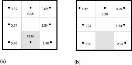
a all eight measurements and their wide variation, giving mean of 3.68 mm and standard deviation of 3.83 mm; b effect of excluding localised corrosion region and associated high reading, resulting in mean of 2.41 mm and standard deviation of 1.45 mm (coupon 15-2A)
Depth of two deepest pits for each coupon/mm
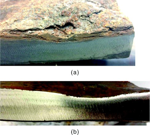
Visual observations
The measurements of depth of corrosion loss did not specifically discern localised or pitting corrosion of cast iron, which is broadly consistent with previous observations in the literature that pitting is not a major issue. 1 However, careful observation of the 34 coupons, and in particular their cut edges, shows that localised corrosion does occur although it does not appear to have the aggressive features normally associated with pitting corrosion of steels. 7 For example, Fig. 6 shows the side of a coupon cut from a pier (15-2A) in the upper tidal zone. The edge shows a depression of the sound metal under the graphitised layer, indicating localised corrosion. For the upper part of the immersion zone, one coupon (13-2C) shows what appeared to be a ‘bubble’ of the graphitised layer. When this was removed, a depression was observed, reflecting the loss of sound cast iron under, as can be seen from the cut edge (Fig. 7a). Removal of all graphitised material revealed what appear to be numerous small pits on the surface of the much larger area of localised corrosion (Fig. 7b). Further down into the immersion zone, approximately half way between the low tide level and the riverbed, somewhat more severe pitting was observed (Fig. 8).
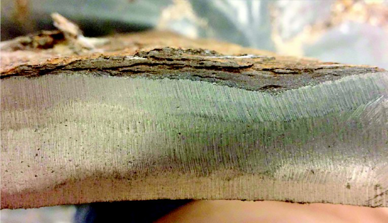
Side of coupon (15-2A) cut from upper tidal zone, showing localised corrosion under graphitised layer and remains of external encrustation (top) (© C. Herron)
a localised corrosion at edge of coupon (13-2C) after removal of upper layer of graphitised material (bubble) [note fractured graphitised material (© C. Herron)] and b edge view similar to a after complete cleaning of coupon, showing evidence of small pits on surface of larger area of localised corrosion (© C. Herron)
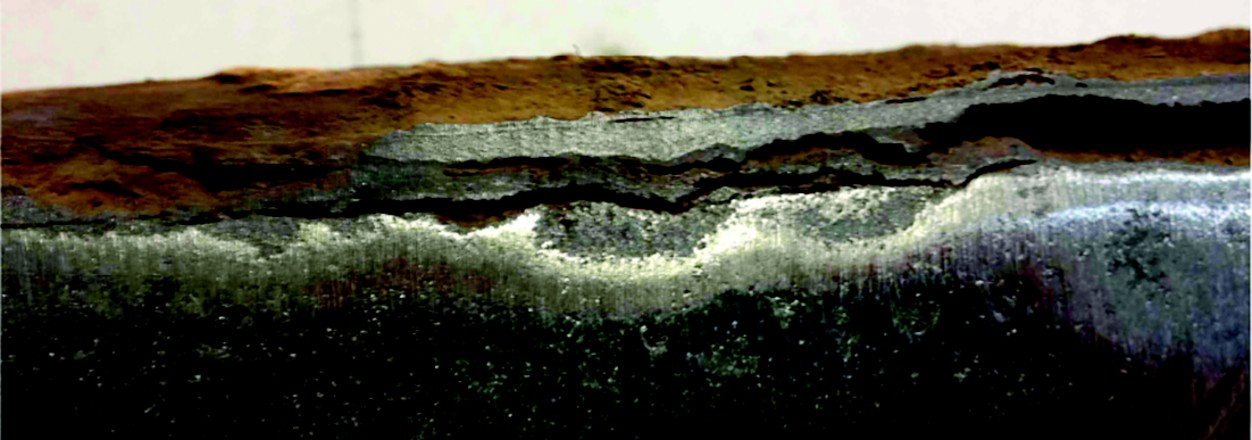
Edge view of coupon 13-2D showing interface region between cast iron (lower), graphitised material (mid) and encrustation (upper); note undulating corroded cast iron surface with pitting apparent and non-uniform nature of graphitised material (© C. Herron)
Analysis of results
Corrosion loss profiles
The overall average corrosion loss results shown in Table 2 can be used to obtain corrosion loss profiles for each of the piers considered in the sampling programme. These are shown in Fig. 9a. The corresponding standard deviations are shown in Fig. 9b. It is seen that, apart from some inevitable variability, the profiles are very similar, with higher than average corrosion just above the mean high tide level and also just below the mean low tide level. The trends seen in Fig. 9 can be made more specific and clearer by considering all the data at any one level across all piers for which corrosion loss measurements were made and determining the averages and the sample standard deviations at each level. The results are shown in Fig. 10.
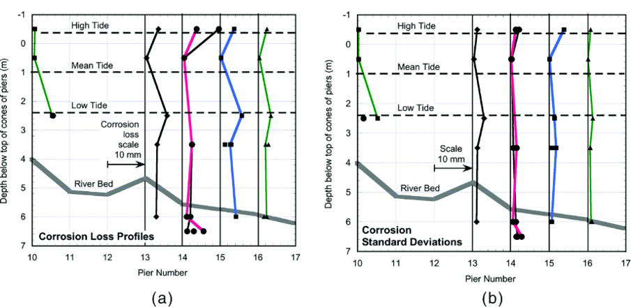
a profiles of average corrosion losses for each pier considered in sampling program (© R. E. Melchers) and b profiles of standard deviation in average corrosion loss for each pier considered in sampling program (© R. E. Melchers)
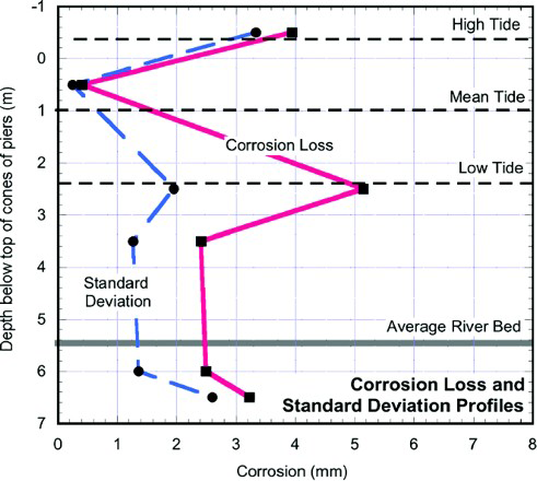
Profiles of corrosion loss and standard deviation averaged for piers 13-16 showing low corrosion at about midtide and high corrosion at high and at low tide levels compared with immersion corrosion (© R. E. Melchers)
It is seen also in Fig. 10 that corrosion losses are high just above the high water mark and are low at the mean tide level, consistent with what has been observed also for steel piles in marine tidal zones. 8 The profiles also show at around the low water level a level of average corrosion (and standard deviation) greater than the corrosion in the immersion zone. Such behaviour has not been observed for steel piling exposed in unpolluted coastal sea waters. 8 Since the completion of the study reported herein, it has been established that, under nutrient pollution conditions, corrosion in the region immediately below the low tide level also can be high, higher than for the immersion zone. 9 This has been termed accelerated low water corrosion (ALWC) and the amount of corrosion in that zone has been closely correlated with elevated levels of dissolved inorganic nitrogen (DIN), a factor known to increase the rate of metabolism of micro-organisms and linked to microbiologically influenced corrosion. 10 The profiles in Figs 9–11 therefore indicate that the tidal waters in which the piers were located were subject to pollution by ammonia, nitrates and possible nitrites, the accepted standard components of DIN. Unfortunately, the water quality of the St Lawrence creek was not sampled at the time of the demolition or, it appears, at any other time. Environmental protection or other authority water quality results also appear not to be available for the catchment. However, historical records for the township of St Lawrence 11 show that, at one time, the town was an important pastoral transit centre, with a throughput of some 100 000 sheep and 40 000 cattle annually. Given also the historical lack of environmental controls, it is possible that there would have been high levels of animal waste runoff into St Lawrence creek waters. Such wastes are high in DIN and other nutrients known to enhance microbiological metabolism and thus to increase the likelihood of microbiologically influenced corrosion. 12
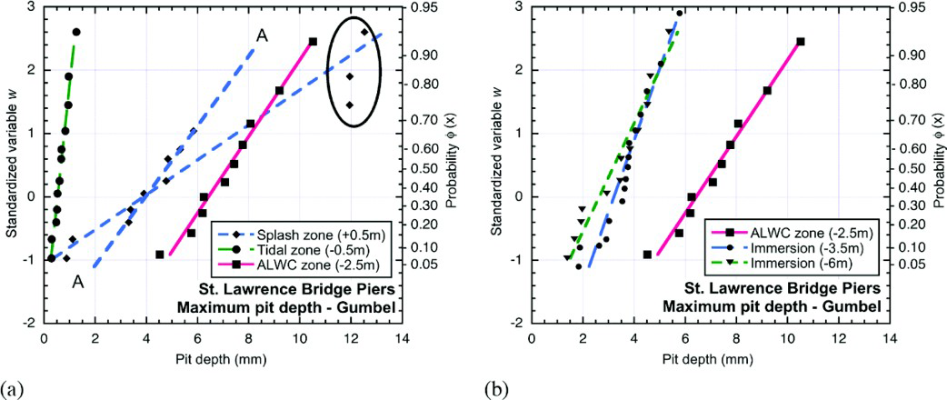
a splash, tidal and ALWC zones; b ALWC and two different levels in immersion zone
Extreme value analysis of maximum pit depths
For analysis of maximum pit depths, it is conventional to use an extreme value analysis of the data. Specifically, the Gumbel extreme value distribution usually is considered appropriate for maximum pit depths 13 and has been applied widely. The approach used here was to select the two deepest pit values for each coupon and assume that each is the deepest pit for a surface area equal to half the size of the coupon. The relatively small variations in coupon size were ignored. At each elevation (from +0.5 to − 6 m), all extreme pit depths were collected to form a statistical sample, sorted in rank order, assigned a cumulative probability using standard procedures 14 and plotted as shown in Fig. 11. For clarity, two plots are shown with the data for the ALWC zone in common.
It is clear from Fig. 11 that, with one exception, each data set can be represented by a linear trend, indicating the Gumbel extreme value distribution is an appropriate representation. For the splash zone, the data set (Fig. 11a) has three data points (circled) that clearly are not consistent with the trending of the rest of the data. That data can be assigned the trend marked A-A. Departures of data points from linearity on a Gumbel plot have been noted before and usually such points are dismissed as ‘outliers’, without being given further consideration. However, given the wide departure from the trend A-A, it appears unlikely that the three circled data points simply are outliers.
Discussion
For extreme value analysis, discarding one or more data points as outliers has been a practice followed for many years.14,15 However, it also has been shown that departures from linearity are not necessarily random and could be the result of physicochemical or other processes affecting corrosion. 16 One possibility is that these values are associated with material defects or inclusions, thereby increasing significantly the starting point or a step in the development of corrosion pitting. As observed earlier for steels, corrosion pitting is likely to progress in stages, with the development of pit depth being limited by potential limitations although this does allow a certain degree of sideways development. 17 As a result, pits tend to amalgamate or coalesce, forming plateaus that then permit new pitting to develop, a pattern that has experimental observational support, at least for steels. 18 A corollary is that any defects or inclusions present anywhere in the matrix of the material can add to faster, temporary development of pit depth. Considering that cast iron is known to be prone to having defects and inclusions in its structure, 5 it is considered feasible that the outliers, circled in Fig. 11a, are the result of such defects or inclusions. If this is correct, it immediately raises the question how this aspect should be considered in any statistical analysis and indeed whether extreme value analysis in the conventional manner of application is applicable. These clearly are matters for further investigation.
Apart from developing probability distributions to represent the probability of occurrence of the depth of the deepest pits, an important matter for structural engineering is the remaining wall thickness and thus the average corrosion loss likely to occur as a function of time. As noted above, very limited data are available for longer term exposures of cast iron in marine environments, and the influence on such corrosion of the parameters involved is not particularly clear. 4 For tropical environments, the corrosion loss observations in PCZ 3 are useful and provide the possibility for extension beyond the 16 year time horizon applicable to those results. However, this can be carried out only for ‘machined’ cast iron coupons as their data extend to 16 years, but for ‘as cast’ cast iron, which is relevant for the present study, the PCZ data sets cover only 4 years. The average sea water temperature in the PCZ is ∼27°C on average, comparable with that at St Lawrence.
The PCZ data is for isolated coupons. In contrast, the results reported herein are for cast iron that is continuous through the tidal zone. Care is required since, for steel strips, corrosion through the tidal zone shows quite different behaviour, particularly in the tidal zone, compared to that for electrically isolated coupons. 8 A similar characteristic can be expected for cast iron since, in both cases, the predominant material involved in the corrosion process is ferrous iron. For steel, the corrosion of isolated coupons and of strips in the immersion zone has been found to be closely similar, and this might be expected also for cast iron. In this case, it is valid to compare the PCZ data for immersion corrosion with the results obtained in the present study. Figure 12 shows the data both from the PCZ tests and from the present investigation for 90 years of exposure.
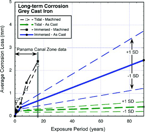
Average corrosion loss data for immersion and for midtide exposures extrapolated from limited data available from Panama Canal Zone (0-4 years) (© R. E. Melchers)
In plotting Fig. 12, it is assumed, for lack of any contrary experimental evidence, and with some support from the PCZ data sets for various metals,2,3 that the long term trends are linear or can be approximated as such. Standard deviation estimates have been added, acknowledging that, for the PCZ, there is no such information.
Figure 12 also shows the observations from the PCZ for corrosion loss for coupons in the midtide (‘tidal’) zone. For such coupons, the corrosion losses usually are relatively much higher than observed at midtide for strips. 8 However, as seen, overall, the losses are still quite low, and thus, this aspect may be ignored in plotting the line for midtide corrosion obtained in the present study. Again, the standard deviations estimated from the present data are shown also.
As noted, for the corrosion profile shown in Fig. 11, the rather high level of corrosion just below the low tide level is likely to be ALWC as a result of elevated concentration of nutrients, mainly DIN, critical for the occurrence and development of microbiologically influenced corrosion in sea waters. It should be borne in mind that the corrosion losses that were observed during the present investigation essentially are the result of a very long period of exposure (some 90 years) to St Lawrence creek waters. It is conceivable that the degree of water pollution, and in particular DIN pollution, will have changed over the life of the bridge piers.
The information presented herein about long term corrosion losses for grey cast iron and the variability in those losses and the evidence that non-uniform corrosion of cast iron can be observed in samples is, as best as can be ascertained, unique in the corrosion literature. Such information is important for the assessment of the current safety of existing cast iron infrastructure such as railway and road bridges. Also important is the prediction of likely future rates of corrosion, and for this, the extrapolation approach outlined herein is considered relevant.
Finally, in the broader context, it is hoped that the exposition given herein will motivate others involved in the demolition of older, perhaps heritage cast iron and also wrought and structural steel structures, to take the opportunity to perform studies along the lines indicated herein. So doing will help increase understanding of long term corrosion behaviour as well as the uncertainties associated with it.
Conclusions
Even in sea water exposure environments such as immersion and in the tidal zone, cast iron corrodes remarkably little over many decades provided that there is little or no pollution of the sea water.
The corrosion profiles for the piers through the tidal zone show a pattern similar to what is known as ALWC for steel piling in polluted sea waters. This indicates that the observed corrosion profiles for the cast iron piers are likely to be the direct result of water pollution of the waters in St Lawrence creek during the life of the bridge. This is consistent with known land use in the river catchment.
The corrosion of cast iron is not ‘uniform’ but may exhibit considerable localised corrosion over areas some 50-100 mm in size with corrosion penetration 6-8 mm more than in the surrounding areas. Some areas of much smaller pitting were observed also.
An extreme value statistical analysis of maximum pit depth data at various elevations through the water column showed close consistency with the Gumbel distribution, except in the case of pitting in the splash zone. It is proposed that the few but considerably deeper pits are partly the result of defects or imperfections or inclusions in the cast iron. A mechanism by which the deeper pitting might come about is proposed.
Footnotes
Acknowledgements
The support of Queensland Rail in provision of coupons and cylinders as part of a consulting activity with SKM [now Jacobs Group (Australia)] is acknowledged. Part of the work reported herein was carried out by C. Herron as part of his final year Civil Engineering Student Honours Project at The University of Newcastle, Australia.