New approach towards dynamic modelling of dephosphorisation in converter process

Abstract

A new approach was made to model the dephosphorisation process in a 300 tons basic oxygen furnace converter with three argon gas inlets. The main feature of the new approach was to utilise the velocity vectors obtained by computational fluid dynamics (CFD) simulation in a standalone model. The CFD simulation was carried out using commercial software COMSOL Multiphysics. In the standalone model, the steel melt domain was sliced into 1000 cells. The calculated velocity vector in each cell was assumed constant. Based on the imported velocity vectors from the CFD calculation, the mass transfer of carbon and phosphorus was calculated by taking into account the slag–metal reactions. The mass exchange between slag and metal was considered to be dominated by the metal droplet formation due to the oxygen jet. The convergence of the model calculation and the promising comparison between the model prediction and the industrial data strongly suggested that the proposed approach would be a powerful tool in dynamic process control. As a preliminary step, the model only simulated the process after the formation of slag–metal–gas emulsion. Note that the present work is intended to establish a structure of the model. More precise descriptions of other process aspects need to be included before the model can be practically employed in a dynamic controlling system.

Introduction

The oxygen steelmaking process, also known as the basic oxygen furnace (BOF) or Linz–Donawitz process, has been around for ∼60 years. With the decreasing access to prime raw materials and the increasing penalties and costs for yield losses and wastes, the need for improved process understanding and more accurate process control is becoming greater. The use of advanced computer models is the key in the development of the next stage of process control tools for oxygen steelmaking.

The importance of bottom blowing in the converter has since long been realised.¹ 1,2 Although the oxygen jet drives the flow of the bath and increases the velocity near the surface, the flow pattern in the liquid metal bath inside the BOF is mostly governed by bottom stirring practice. One of the primary tasks in the converter is dephosphorisation. Choudhary and Ajmani3 have reported that the argon stirring in the converter has substantial impact on phosphorus partition. Optimisation of the argon stirring can improve the dephosphorisation considerably. On the other hand, it is well known that the blockage of the gas inlets when the converter is becoming old will strongly affect the argon flowrate. The decrease in gas flowrate might slow down the dephosphorisation reaction.

In view of the impact of the flow pattern on the converter process, many computational fluid dynamics (CFD) modelling studies have been conducted.4 ^– 6 For example, a very comprehensive CFD modelling study has been carried out by Odenthal et al.4 They studied the fundamental flow phenomena, such as the penetration of supersonic oxygen jets, the motion of phase interfaces and the behaviour of gas plumes. In fact, the CFD model has proved to be a powerful tool to predict the flow in the reactors for metallurgical processes. Unfortunately, despite the success of CFD in the calculation of flow, mass transfer and heat transfer, it is still impossible to incorporate CFD directly into any online process modelling due to the complicated nature of the processes and the limitation of the CFD software.4 More or less, the calculation is still at the stage of studying the relative trend of the process and providing suggestions.

The demands of energy saving on the efficiency of the process and better process control have stimulated the developments of new techniques, e.g. acoustic measurement, infrared detection and off gas measurements. These techniques have prepared the steel industry for accurate dynamic control as they provide reliable feedback signals. Unfortunately, most of the existing dynamic control models are still based on statistical analysis. The nature of this type of model makes it difficult to meet the need for new process modification and the application of the model to other steel plants.

The present work aims at a new approach towards the development of dynamic models for process control in BOF. It utilises the velocity vectors calculated by CFD simulation to calculate the mass transfer in the metal bath. The calculation provides the concentrations of carbon and phosphorus at the slag/metal interface as a function of blowing time. A model for slag–metal reaction has also been developed to take into account the concentration variation due to slag–metal reaction. The foremost focus of the present work is to examine whether the use of CFD results in a standalone model can become potentially a process model that controls dynamically the operation using the feedback information.

Overall model consideration

Mass transfer in liquid metal

As mentioned in the section on ‘Introduction’, while the CFD calculations can suitably describe the fluid flow in the reactors, it is still almost impossible to incorporate the CFD calculation directly into any process model. The present approach intends to utilise the powerful CFD tool to predict the flow velocities in the converter. The calculated velocity vectors can be used to calculate the mass transfer (and even heat transfer) in liquid steel since the diffusion in the liquid phase is negligible in a gas stirred bath. To calculate the mass transfer in a standalone model, or later in a process model, the domain in the liquid metal is sliced into small cells. The net mass flux into a particular cell (mass in minus mass out) can be well calculated at a given moment using the calculated velocity vectors.

Slag–metal reactions

Chemical reactions in the converter process are very complicated. In fact, it takes 3–5 min before a liquid slag is built up. In this period, silicon is oxidised first due to its high affinity to oxygen. Oxidation of iron and manganese by oxygen gas will also take place to meet the constraints of mass balance. Even some carbon can be oxidised in this period, though the reaction does not dominate. Lime is dissolved in the initial slag throughout this period. Thereafter, a liquid slag containing mostly CaO, FeO, SiO₂, MnO and MgO is formed. The impinging of the oxygen jets on the liquid surface results in an emulsion consisting of slag, liquid metal droplets and gas bubbles. It is reasonable to expect that the reaction rate of decarburisation and dephosphorisation is dominated by the reaction between the metal droplets and the foaming slag, since a few tons of droplets per second are thrown into the slag.7 ^– 9 The droplets stay in the slag a few seconds before returning to the metal bath.

As the first step towards dynamic process control, the present model would start at the moment when the initial slag and the slag–metal–gas emulsion have formed (∼3 min after the start of blowing). The following considerations are made, and the assumptions are made correspondingly.

First, the model only simulates the process after the formation of slag–metal–gas emulsion. The period of initial slag formation will be studied later.

Second, the composition of the slag still varies even after the formation of the slag emulsion. Because of the insufficient transport of carbon to the slag/metal interface, more iron is oxidised in the earlier stage, leading to a high FeO content in the slag. The FeO content decreases after this period. This aspect is well known and illustrated in Fig. 1, which is reproduced from the publication of Jalkanen and Holappa.10 The figure shows also that the slag composition does not vary significantly after this period (∼40% blowing). Some publications report the variation in FeO content.11 On the other hand, the variation range of FeO is not very large, as reported by Cicutti et al. 11 at between 15 and 25 mass-%. Note that the variation in the slag composition has to be taken into account in a real dynamic process model. However, to simplify the present model, which is the first step of the dynamic modelling approach, the slag composition is taken as constant after the initial periods. In view that the slag composition is mostly used to evaluate the activities of P₂O₅ in the slag and the oxygen activity in the steel droplets, this assumption will not affect the model calculation substantially in the preliminary model.

Figure 1.

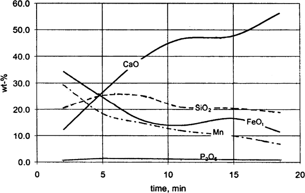
Slag evolution in converter reproduced from Jalkanen and Holappa10

Third, there are a couple of mechanisms for the decarbonisation reaction. Since the interface area between the droplets and the slag in the emulsion is much bigger than the area of the metal surface in the bath, the rate of decarbonisation is considered to be mostly due to slag–droplet reaction. The reaction can be expressed as (1) where the activity of [O] is governed by reaction (2) (2) A previous study12 has shown that the concentration gradient in the steel droplets is negligible. Droplets having diameters of >0·4 mm have the same carbon content at a given moment in the emulsion.13 These two facts strongly suggest that the metal droplets are in equilibrium with the slag and the gas phase in the emulsified slag. It is also expected that the steel at the slag/metal interface is in equilibrium with the slag. Hence, the calculated instant [C] for slag–metal equilibrium by equation (1) is justified. The partial pressure of CO gas is assumed to be 0·8 based on the industrial data of off gas analysis.

Fourth, the dephosphorisation reaction is also dominated by the reaction in the slag–metal–gas emulsion. This reaction can be described as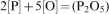 (3) Fifth, the amount of metal droplets thrown into the slag emulsion per second is a function of the oxygen flowrate and the height of the lance.7 In this work, constant oxygen flowrate and lance height are assumed to simplify the situation. Future work must be carried out to obtain the rate of droplet formation.

Sixth, since the metal droplets are found to be in thermodynamic equilibrium with the foaming slag, it can be assumed that the metal droplets have the same composition as the liquid steel at the slag/metal interface before they are thrown into the slag, and they are in equilibrium with the slag when they fall back to the steel bath at a given moment.

Seventh, the concentrations of carbon and phosphorus vary with blowing time and position in the converter. The concentrations at the slag/metal interface also vary. In addition to the variation due to mass transfer from the lower part of the metal bath, the droplets falling back from the foaming slag also contribute to the concentration variations at the slag/metal interface.

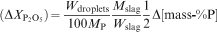
Eight, to simplify the calculation, the contents of the oxide components, except P₂O₅, are assumed constant throughout the process. The flux of phosphorus from the metal droplets to the slag is calculated by the following thermodynamic constraint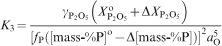 (4) where is the mole fraction of P₂O₅ at the previous step, is the change in mole fraction of P₂O₅, [mass-%P]^o is the mass percentage of P in the metal droplets before they come into the slag, Δ[mass-%P] is the change inf P in the droplets after reaction with the slag and a _o is the oxygen activity in the metal droplets. can be related to Δ[mass-%P] by the mass balance of reaction (3), i.e. (5) where W _droplets is the weight of the metal droplets, W _slag is the weight of the slag and M _P and M _slag are the molar weights of P and slag respectively.

The use of equation (3) requires the activity coefficient of P₂O₅. Turkdogan14 has critically reviewed the existing experimental data and presented the following empirical equation for the activity coefficient of P₂O₅ in the converter slag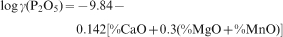 (6) The standard Gibbs energy (J) for reaction (3) is obtained from the literature15 (7)

Model structure

The abovementioned facts are summarised in Fig. 2. The figure also schematically illustrates the model structure:

Figure 2.

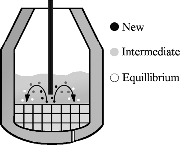
Schematic illustration of present model

the velocity distribution in the metal is calculated by CFD modelling; the velocity is constant in each calculating cell

ii.

the oxygen potential increases in the initial stage of the slag formation and becomes nearly constant thereafter; the oxygen activity can be evaluated by reaction (2)

iii.

a certain amount of metal droplets (kg s⁻¹) is thrown up into the foaming slag by the oxygen jet

iv.

the metal droplets have reached equilibrium with the slag with respect to P before they fall back to the liquid metal. Note that a certain amount of Fe droplets will get oxidised into FeO and dissolved into the slag. However, since the increase in FeO content in the slag (see Fig. 1) is not substantial, it is reasonable to assume in this preliminary model that the amount of metal droplets falling back to the liquid metal bath is the same dynamically as the amount thrown up by the oxygen jet

the liquid metal in a given cell at the slag/metal interface reaches a new composition after each time step due to the mass exchange with the neighbour cells and the exchange of metal droplets with the slag. The calculation is made step by step repeatedly.

Computational fluid dynamics calculation

In view that many CFD models can be found in the literature, only a brief description of the model is given here to orient the reader.

The three-dimensional model of the 300 tons BOF vessel (see Fig. 3) consists of one domain with three inlets. The vessel has a diameter of 6 m, and the metal bath height is 1·5 m. The positions of the three gas inlets, located on a half circle at a radius of 1·65 m, are also marked in Fig. 3.

Figure 3.

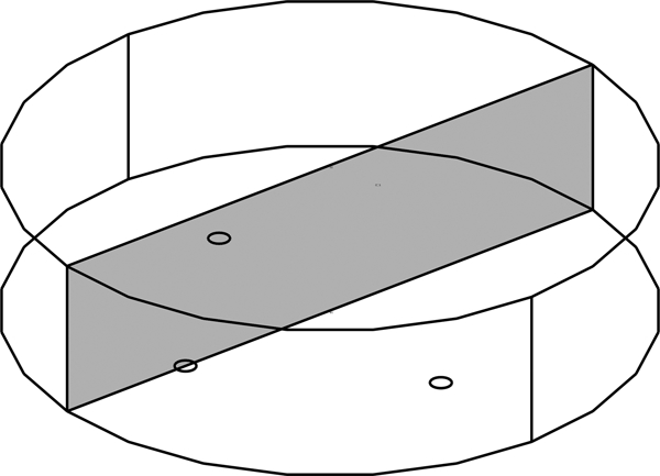
Simulating domain of BOF vessel

Governing equations

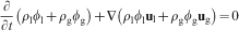
All the governing equations are taken directly from the COMSOL Multiphysics 3·5 Chemical Engineering module. The bubbly flow model is utilised to calculate the flow induced by argon stirring. The bubbly flow model is a two-phase model, with each phase having a separate velocity field. The momentum equation is expressed as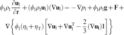 (8) The continuity equation is expressed as (9) where φ is the fraction of either phase, ρ is the density (kg m⁻³), p is pressure (Pa), g is the gravity force and u is the velocity vector (m s⁻¹). The subscripts l and g stand for liquid and gas phases respectively. η _l and η _T in equation (8) denote dynamic and turbulent viscosities respectively. The K–ϵ model is employed to calculate turbulent flow.

It is well known that the flow field in the liquid metal is driven mostly by bottom blowing;16 only the flow near the surface region is affected by top blowing. Since the focus of the present work is the mass transfer in the bath, only bottom stirring is considered. The following assumptions are made:

the temperature is constant throughout the model. This assumption is justified by the fact that the forced convection due to stirring is the dominant factor. It should be pointed out that the local heat generation by the gas–metal reaction is substantial. Considering that the flow is still mostly due to the forced convection, this heat generation is left for later modelling effort to study

ii.

the density and dynamic viscosity are assumed to be constant, with the former being 7000 kg m⁻³ and the latter 0·007 Pa s

iii.

the top slag is not considered in the fluid flow calculation; the surface is assumed to be flat

iv.

the gas flowrates going through the three gas inlets are the same and constant throughout the entire calculation time.

Boundary conditions

The following boundary conditions are adopted:

logarithmic wall function is used for the walls

ii.

the walls are insulating for the gas phase

iii.

a gas flux (kg m⁻² s⁻¹) is used for each gas inlet to get the correct flowrate (N m³ h⁻¹)

iv.

the steel surface boundary is set to outlet for the gas phase.

Computing and results

A tetrahedral mesh consisting of roughly 20 000 elements is employed. The Paradiso solver is used. The fluid flow is solved in transient mode with a solution time of 300 s. The solution at 300 s is used as the initial condition for a stationary solution.

Three total gas flowrates were studied, namely 400, 600 and 800 N m³ h⁻¹. As examples, Fig. 4 presents the flow patterns at the vertical section through the middle gas inlet for the three flowrates. This section is marked in Fig. 3 to help the reader. Note that the velocity arrows only consist of the two components in the vertical section. The flow patterns are very similar for the three gas flowrates. It is seen that the liquid metal is brought up by the gas plumes. The liquid travels downwards along the wall far from the gas inlet. It is also seen that the increase in the total gas flowrate from 400 to 800 N m³ h⁻¹ does, in general, increase the velocity. An increase of ∼20% is observed in the metal–gas plume when the gas flowrate is doubled. On the other hand, the increase is not very profound in the remaining parts of the bath.

Figure 4.

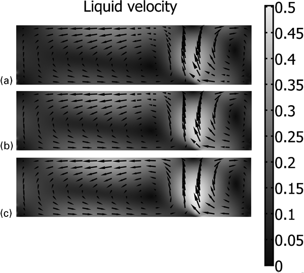
Flow profile through centre inlet at a 400 N m³ h⁻¹, b 600 N m³ h⁻¹ and c 800 N m³ h⁻¹

Dynamic model

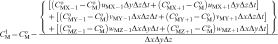
To construct the model, the domain of the liquid metal is sliced into 1000 cells (10×10×10). The velocity vectors obtained at the centres of the cells by CFD calculation are imported to the 10×10×10 domain. At the start of the calculation, the concentrations of either C or P in all the cells are assumed to have the same initial value. Figure 5 illustrates how the net flux into a particular cell Cell_M is considered.

Figure 5.

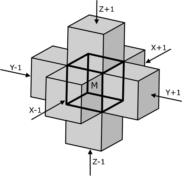
Illustration of fluxes from neighbouring cells

The concentration (of either C or P) in Cell_M after a time step can be calculated by the following equation using the concentrations of the neighbour cells at the previous step (10) where the subscripts are used corresponding to the cells marked in Fig. 5; the superscripts o and 1 stand for the previous and present steps. In equation (10), u, v and w denote the velocities in the x, y and z directions respectively. It must be noted that only the fluxes towards Cell_M are considered in equation (10). The u, v and w values are taken as positive when the fluxes are towards Cell_M. They are set to zero when the fluxes are in the outward direction from Cell_M. In other words, the fluxes going away from Cell_M are taken into account only when the corresponding neighbour cells are considered.

As mentioned earlier, in the initial period of blowing, only a limited amount of carbon is oxidised. Carbon starts decreasing when most of the silicon has been oxidised. Because of the low oxygen activity in the hot metal, the dephosphorisation is expected also to be very limited during this period. Hence, all the simulations are carried out 180 s after the start of blowing.

The FeO content varies in the first 8–10 min. Thereafter, the FeO content is somewhat constant. In the present work, the slag composition in the second half of the process is assumed to be 51CaO–15SiO₂–5MgO–24FeO–5MnO (mass-%).11 Calculation using the thermodynamic model17 reveals that the oxygen activity in the metal droplets is ∼0·0885. It is also assumed that the oxygen content increases linearly with time before it reaches this value (11) The initial composition of the liquid metal is given in Table 1. The weights of liquid metal and slag are also listed in the table. The amount of droplets thrown up to the slag depends on the oxygen flowrate and the lance position.7 Subayago and his co-workers8 have derived a dimensionless number, the ‘blow number’. The amount of droplets formed and estimated using this dimensionless number varies between 800 and 2000 kg s⁻¹, depending on the size of the reactor, the gas flowrate and the height of lance. Hence, the total weight of metal droplets thrown up by the oxygen jet is assumed to be 2000 kg s⁻¹. The calculations for droplet formation of 800, 4000 and 6000 kg s⁻¹ are also made for discussion.

Table 1.

Data used for model calculation

Steel and slag mass	Steel: 300 000 kg
Steel and slag mass	Slag: 30 000 kg
Initial chemical composition of steel	4·7C–0·5Si–0·4Mn–0·1P–0·05S and 60 tonnes of scrap (0·5C–0·05Si–0·5Mn–0·02P–0·05S)
Initial chemical composition of slag	51CaO–15SiO₂–5MgO–24FeO– 5MnO (mass-%)

A simple Windows software is developed to conduct the calculation. The stepping speed is 0·7 steps/s.

Results and discussion

The concentrations of C and P in the metal bath are calculated after each stepping time. As an example, Fig. 6a presents the concentration distributions of carbon in the vertical section through the central gas inlet (the section is marked in Fig. 3) after 600, 750 and 900 s. For these calculations, a total argon flowrate of 800 N m³ h⁻¹ is employed. The corresponding phosphorous concentrations at the same blowing times are presented in Fig. 7. It is seen that the concentration gradients for both C and P decrease with blowing time. The concentration profiles are in good accordance with the velocity distributions shown in Fig. 4. The metal–gas plumes brought up the liquid metal to the slag/metal interface. After the reaction with the slag, the metal flows downwards along the wall far away from the gas–metal plumes. Consequently, the concentrations of C and P show higher values on the left side, where the metal goes up, and lower values when the liquid metal goes downwards along the opposite wall. This phenomenon is more profound in the earlier stages of decarburisation (see Fig. 6a ) and less when most carbon and phosphorus are taken away (see Fig. 6c ).

Figure 6.

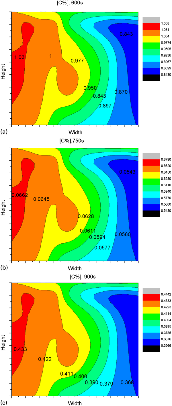
Carbon distributions on central slice at a 600 s, b 750 s and c 900 s

Figure 7.

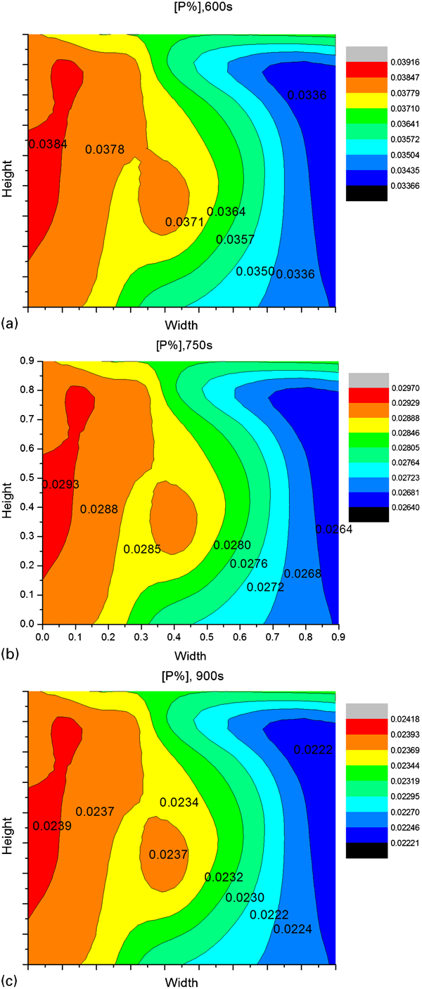
Phosphorous distribution on central slice at a 600 s, b 750 s and c 900 s

Figure 8 presents the variations of the average carbon concentration with time for three different argon flowrates. Similarly, the variations of the average phosphorus concentration at different argon flowrates are presented in Fig. 9. Although the curves are very close to each other in both ^{Figure 8} Figs. 8 and 9, the stirring does have a very strong impact on decarburisation and dephosphorisation, especially at the late stage of the process. For example, if the process requires a phosphorus concentration of 0·02 mass-%, the reduction in argon flowrate by 50% would prolong the dephosphorisation time considerably. The lower the requirement of the phosphorus content, the longer the stirring time needed for the lower argon flowrate. As shown in Fig. 9, to reach the goal of 0·02 mass-%P, the time for 75% argon blowing would increase by >200 s, while the time for 50% argon would be even longer. This result is in line with the industrial observation that the dephosphorisation is not so efficient when the converter becomes old. The partial blocking of the gas inlets that leads to much lower argon flowrate is a good explanation for the reduced dephosphorisation power.

Figure 8.

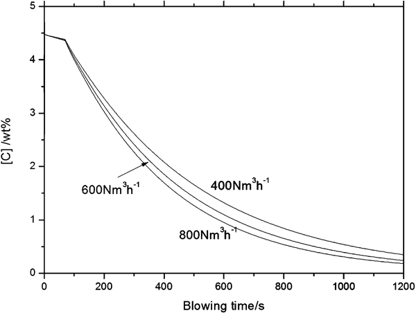
Variation in [C] with blowing time at different argon flowrates

Figure 9.

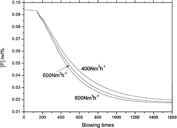
Variation in [P] with blowing time at different argon flowrates

Cicutti et al. 11 have reported the concentrations of carbon and phosphors at different blowing times for a converter of 200 T. The sampling position is very close to the slag/metal interface. Although their results are obtained from a different converter, it is still interesting to make a relative comparison with the present model prediction. This composition is shown in Fig. 10a for carbon and Fig. 10b for phosphorus. Since no exact sampling position but only a figure is given in the paper, the position is estimated. The concentrations shown in the two figures are calculated at this corresponding position. It is seen in Fig. 10a that the predicted curve using 2000 kg s⁻¹ droplet formation agrees with the experimental data reasonably well. On the other hand, the experimental data for P in Fig. 10b show a much faster dephosphorisation rate than the model prediction. Note that P reaches almost the equilibrium value in the melt after 200–250 s of blowing. In view that such a low P content would require a very high oxygen potential in the melt and the oxygen potential is still very low at this moment, the experimental data might be subjected to certain uncertainties. This aspect will need further study. The generation rate of metal droplets of 2000 kg s⁻¹ seems to predict the decarbonisation quite well. Using 2000 kg s⁻¹ for the droplet, the generation rate is on the higher side of the droplet formation. Even this aspect needs careful study in order to develop a dynamic model with high precision.

Figure 10.

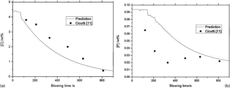
Comparison of model prediction with industrial data from Cicutti et al. 11

It must be pointed out that the present work does not focus on the precise modelling of a particular BOF reactor. Instead, the aim is to develop a structure of the future dynamic process model, which can utilise CFD results. The convergence of the model calculation, along with the semiquantitative comparison between the model prediction and the experimental data (see Fig. 10), suggests that the present modelling approach could be a promising route for the dynamic controlling model in the real process.

Note also that the present modelling exercise can only be considered as a preliminary but pioneer attempt of using the results of CFD calculations in a real process model. In order to reach the goal of a real dynamic controlling model, many aspects need to be improved and considered. The following aspects are the foremost factors to be considered in the next step along the present line:

the slag composition needs to be modelled as a function of the blowing time

ii.

the amount of droplets thrown up to the slag needs to be modelled as function of the oxygen flowrate and the position of the lance

iii.

droplets could even be oxidised into FeO dissolving in the slag. This will not only affect the mass balance calculation but also vary the slag composition. Hence, this point should be modelled simultaneously with point (i)

iv.

the oxidation of C by the oxygen gas at the gas/metal interface needs to be included

the thermodynamic model to estimate the activity coefficient of P₂O₅ needs a careful study for the real converter slag.

Summary

The present work proposes a new model structure towards the development of dynamic models for process control in the BOF. It utilised the velocity vectors calculated by CFD simulation to calculate the mass transfer in the metal bath. The standalone model provides the concentrations of carbon and phosphorus at the slag/metal interface as a function of blowing time. A model for slag–metal reaction was also developed to take into account the concentration variation due to slag–metal reaction. The foremost focus of the present work is to see whether the use of CFD results in a standalone model can potentially become a process model, which controls dynamically the operation using the feedback information.

It must be pointed out that the present work did not focus on the precise modelling of a particular BOF reactor. Instead, the emphasis was to develop a structure for a future dynamic process model. The convergence of the model calculation along with the semiquantitative comparison between the model prediction and the experimental data suggested that the present modelling approach could be a promising route for a dynamic controlling model in the real process. A significant amount of modelling work taking details of the process is still required before the model can be employed in dynamic process control.

References

Baker

Normanton

Spencely

Atkinson

: Ironmaking Steelmaking, 1980, 7, (5), 227–238.

Chatterjee

Marique

Nilles

: Ironmaking Steelmaking, 1984, 11, (3), 117–131.

Choudhary

Ajmani

: ISIJ Int., 2006, 46, (8), 1171–1176.

Odenthal

H.-J

Falkenreck

Schlüter

: Proc. European Conf. on ‘Computational fluid dynamics’, Delft, The Netherlands, September 2006, TU Delft. 220–241.

Olivares

Elias

Sánchez

Díaz-Cruz

Morales

: Steel Res., 2002, 73, (2), 45–51.

Ersson

Höglund

Tilliander

Jonsson

Jönsson

: ISIJ Int., 2008, 48, (2), 147–153.

van der Knoop

Deo

Snoeijer

van Unen

Boom

: Proc. 4th Int. Conf. on ‘Molten slags and fluxes’, Sendai, Japan, June 1992, Iron and Steel Institute of Japan, 302–308.

Brooks

SubayagoGA

Coley

Irons

: ISIJ Int., 2003, 43, (7), 983–989.

Dogan

Brooks

Rhamdhani

: ISIJ Int., 2009, 49, (1), 24–28.

10.

Jalkanen

Holappa

: Proc. 7th Int. Conf. on ‘Molten slags, fluxes and salts’, Cape Town, South Africa, January 2004, The South African Institute of Mining and Metallurgy. 71–76.

11.

Cicutti

Valdez

Pérez

Petroni

Gómez

Donayo

Ferro

: Proc. 6th Int. Conf. on ‘Molten slags, fluxes and salts’, Stockholm, Sweden/Helsinki, Finland, Royal Institute of Technology, June 2000. 367.</vol>

12.

Thoren

: Personal communication, SSAB Oxelösund AB, Oxelösund, Sweden.

13.

Frenning

: PhD thesis, A Study of Top Blowing with Focus on the Penetration Region, Royal Institute of Technology, Stockholm, Sweden, 2010.

14.

Turkdogan

: ISIJ Int., 2000, 40, 10, 964–970.

15.

Turkdogan

Pearson

: J. Iron Steel Inst., 1953, 175, 393.

16.

Singh

Ghosh

: Ironmaking Steelmaking, 1990, 17, (5), 333–342.

17.

Björkvall

: PhD thesis, Thermodynamic study of multicomponent slags, Royal Institute of Technology, Stockholm, Sweden, 2000.