
Abstract
Analysis of a single strand 36 t thin slab caster tundish has been conducted with different sets of furniture using a three-dimensional computation fluid dynamics model taking heat losses into account. Five distinct and optimised cases and a base case were used for simulation. The cases were built considering tundish furniture that is readily and economically available and provides ease of maintenance, thus targeting an optimal set of furniture. The performance of different sets of furniture was assessed based on residence time parameters like plug volume fraction, mixed volume fraction, dead volume fraction, etc. Other performance indicators used in the analysis were temperature distribution, observing cold spot, surface velocity and nature of flow in the tundish. Insight from the base case reveals the desired flow characteristics that help to achieve the target performance. Inferred results suggested the use of a turbulence inhibitor in combination with a dam as the optimal set of furniture. Use of a non-isothermal model is important, as it was found that even a small change in temperature (2·3°C) plays a vital role in the fluid flow inside the tundish.
List of symbols
mass fraction of injected tracer
empirical constant ( = 9·793)10
acceleration due to gravity
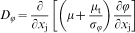
turbulent kinetic energy
turbulent kinetic energy at point p to the wall
length of the tundish
pressure
time
mean velocity
mean velocity at the cell centre adjacent to the wall

average turbulent stress
width of the tundish
coordinate for measure of distance
distance from point p (adjacent to wall) to the wall
rate of dissipation of turbulent kinetic energy
von Karman constant ( = 0·4187)
co-efficient of viscosity
density of the fluid
co-efficients
either k or ϵ
Subscripts
ith or jth component in three Cartesian coordinate directions x, y and z
turbulence
effective
Introduction
The steelmaking tundish is the last point for improving steel cleanliness before casting. To achieve better tundish performance, different types of furniture are used along with suitable tundish design. It is well established that a good performing tundish should have a minimum dead volume fraction (DV), short circuiting flow, heat loss and slag entrapment while maximising plug flow fraction, optimised surface directed flow and, of course, good inclusion removal.1 – 8 An appropriate use of tundish furniture helps to achieve the abovementioned goals but at the same time increases the cost of refractory lining and downtime for maintenance. Moreover, continuous development in the field of tundish furniture has generated vast varieties of furniture to choose from.8 – 13 This increases the complexity in terms of the right choice so as to strike the right tradeoff between tundish performance and cost. Hence, for any new plant set-up, this gives an opportunity for a tailormade solution. For an upcoming single strand thin slab caster at Tata Steel, tundish furniture is a matter of optimal choice. Given the Tata Steel experience in running tundishes for billet and slab casters, the study is conducted to arrive at an optimal tundish furniture for single strand thin slab caster tundish.
Traditionally, residence time distribution (RTD) data have been used to quantify the flow characteristic in a tundish, as this distribution can readily be obtained from a well instrumented water model and can also be obtained from plant trials through, e.g. Cu tracers and more recently from validated computation fluid dynamics simulations. Different flow characteristics are obtained from the RTD curve; these quantities include minimum residence time (MRT), average residence time (ART), peak residence time (PRT), DV, plug flow volume fraction (PV) and mixed flow volume fraction (MV). Some of these parameters also correlate with the inclusion distribution in the product. For example, increasing the MRT allows more time for inclusions of particularly small sizes to float out; therefore, a high MRT may correlate with a low inclusion count in the caster mould. Moreover, other quantities derived from fluid flow computation, such as surface velocities and temperature distribution, help in getting insight about the slag entrapment that may exist within a tundish.
In this work, a three-dimensional non-isothermal modelling of single strand tundish flow operation was carried out to analyse its performance with furniture. Different types of furniture combination have been investigated to explore the right tradeoff for performance, ease of use, less material usage, etc. Residence time distribution analysis, surface velocity profile and temperature distribution have been used as performance indicators.
Methodology
Figure 1 shows the symmetrical half of a single strand thin slab caster tundish with typical furniture set having two dams and a weir. Molten steel is poured into the tundish through the shroud submerged in the molten steel in the tundish. The flow of molten steel into the tundish creates enormous turbulence around the pouring point, so to minimise turbulence around the pouring point, different sets of furniture may be used.
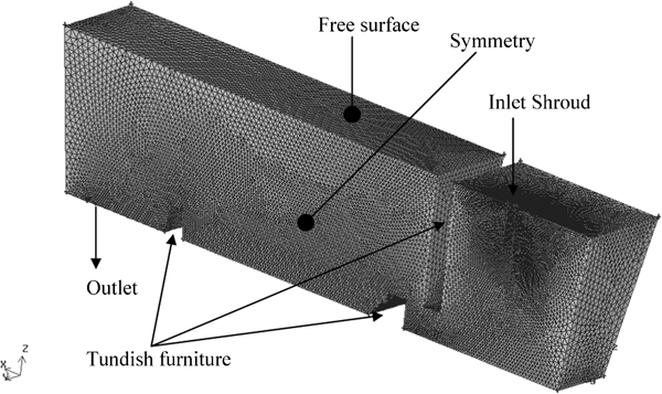
Symmetry tundish geometry and mesh
This dam–weir combination virtually splits the tundish into two parts, confining most of the turbulence within the first part, whereas a dam is provided near the outlet to avoid short circuiting of liquid stream to the outlet along the bottom of the tundish.
Five different combinations of the furniture cases were simulated to investigate the tundish furniture performance. The furniture with two dams and a weir was used as base case to compare any alternate furniture. All the design and operating parameters for the tundish are shown in Table 1.
Design and operating parameters of tundish
Mathematical model
Mathematical formulation and assumptions
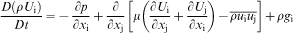
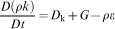
The tundish was assumed to be operating under the quasi-steady state condition non-isothermally with a flat and slag free top surface maintained at a constant level. As in the plant, thermal effects were taken into account by assuming a constant heat flux through refractory walls. The standard k–ϵ model was used to model the turbulence.9 The wall of the tundish was simulated to be hydrodynamically smooth. It was assumed that a local equilibrium exists between the dissipation and production of turbulence at the nearest cell centre wall. The production of kinetic energy and its dissipation rate at the wall adjacent nodes, which are the source terms in the kinetic energy equation, were computed on the basis of the local equilibrium hypothesis. Under this assumption, the production of turbulence kinetic energy and its dissipation rate are assumed to be in equilibrium in the wall adjacent control volume. The following governing equations in tensor form are solved to simulate the flow in the tundish.
Continuity equation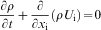
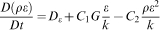


The values of constants used are C 1 = 1·44, C 2 = 1·92, σ c = 1·0, σ k = 1·0, σϵ = 1·3 and Cμ = 0·09.
For the computation of the RTD, the theoretical residence time is given by τ = volume of tundish/volumetric flowrate, and the ART is given by
The MRT is the time when first tracer appears at the outlet, while the PRT is the time when peak concentration is observed at the outlet.
The fraction of dead volume is
Boundary conditions
An overview of the boundaries can be seen in Fig. 1. The inflow of molten steel from the shroud into the tundish was modelled by defining a velocity inlet condition. For simulating actual operating conditions of the plant, the velocity perpendicular to the free surface was calculated using data of the ladle weight and the outflow from the tundish. A medium turbulent intensity of 4% was set at the inlet. To ensure overall mass balance in the tundish, an equal outflow condition from the outlet was set. A no slip boundary condition was applied at all the walls of the tundish and furniture. The standard wall function was used as proposed by Launder and Spalding.14 A symmetry condition was applied at the symmetry plane by putting the gradient of velocity components to zero. At the free surface, zero shear stress boundary condition was applied.
To simulate heat loss from tundish, heat flux boundary conditions were applied. Outflow heat fluxes of 1·96, 4·48, 5·32 and 21 kW m−2 were used for bottom, longitudinal vertical, transverse vertical walls and free surface radiation respectively.15 Adiabatic condition was applied for shroud and internal furniture. The inlet temperature of 1823 K was used for the incoming liquid steel.
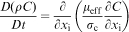
For the tracer dispersion equation, apart from the above boundary conditions, it was considered that all the walls were impervious to the tracer, i.e. at all the bounding surfaces, a zero flux condition was put. The inlet boundary condition of the tracer mass fraction was devised, and a certain amount of tracer was injected for 1 s initially.
Solution methodology
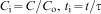
A symmetrical half of the tundish was considered for the simulation. Tundish geometry creation and grid generation were performed using the software Gambit, while the governing equations were solved in the computation fluid dynamics software Fluent, which uses a finite volume technique.16 To ensure the correct implementation of the wall function approach used in the turbulence modelling, the mesh sizes were optimised such that the y + value remains in the 30–90 range, where the logarithm law of wall is valid. The second order upwind scheme was adopted for the convective term in the governing equations. The semi-implicit method for the pressure linked equation algorithm was used to refosolve the pressure–velocity coupling in the momentum equation. 14 14,17 The grid density was kept comparatively high near the inlet due to high velocity gradients there. The solution was assumed to have converged when the whole field normalised residuals for all the variables (U i, p, k and ϵ) fell below 10−4. Values of 7000 kg m−3 and 0·00648 kg m−1 s−1 respectively were used for the density and dynamic viscosity of molten steel. Temperature dependence of density was achieved by Boussinesq approximation. To get the RTD, tracer dispersion equation (equation (8)) was solved. For the solution of the tracer dispersion equation, a time step of 1 s was used to proceed in time after steady state solution for the flow was achieved. The outlet concentration data of the tracer were captured until twice the theoretical residence time. Outlet concentration data and time were made dimensionless as per equation (10).
Validation of the model may be found elsewhere.18
Results and discussion
The simulations were carried out with and without heat loss to assess the role of non-isothermal condition on fluid flow within the tundish. It was found that due to heat loss from refractory walls, the steel temperature drops enough to create a buoyancy effect, which in turn also impacts the RTD. Hence, all simulations were performed with the non-isothermal condition, i.e. taking heat losses from tundish into account. The plant generally operates at varying throughput. To model the different sets of furniture, an average inlet velocity of 1·7 m s−1 was used; this velocity corresponds to the rated capacity of the plant.
Role of heat loss from tundish
To model the thermal effects on the RTD, the heat loss from the tundish was taken into account and compared with the isothermal base case, although the heat loss from tundish is negligible (∼0·17%) in comparison to the incoming heat flux in the form of liquid steel. This results in a temperature drop of 2·3°C from inlet to outlet. Even this small temperature drop causes a strong buoyancy effect in the tundish as comparatively hotter steel enters into the tundish during most of the operation. This phenomenon changes the fluid flow within the tundish, hence RTD. The effect of heat loss on fluid flow is shown in Fig. 2. It can be seen from the figure that liquid steel forms a circulating pattern in the middle of the tundish. In the case of an isothermal tundish, the eye of the circulation is at the centre of the tundish, whereas in the case of a non-isothermal tundish, the eye shifts upward. The reason for the change in fluid flow lies in the buoyancy effect caused by the incoming hotter liquid steel. As fluid comes out of the dam–weir chamber, it moves towards the meniscus, and due to the lesser density, it tries to remain in the top region. Owing to the change in fluid flow, the RTD characteristics of the tundish also get impacted. For the two cases, RTD results are compared in Fig. 3. The RTD analysis reveals a double peak formation, which is characteristic of a wider tundish,19 i.e. W/L>0·17. The extent of short circuiting is more in the case of an isothermal tundish than that of a non-isothermal tundish. This can be seen from the higher first peak in the case of the isothermal tundish. The RTD analysis reveals that comparatively more mixed volume fractions become active in the non-isothermal tundish, as dead and plug volume fractions reduce from 15 and 25 to 9 and 22% respectively, while mixed volume fraction increases from 60 to 69%. The pronounced thermal effect makes it mandatory to take the thermal effect into account for tundish simulation.
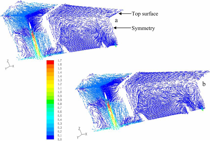
Velocity vectors (m s−1) at symmetry and top surface
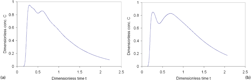
Comparison of RTD characteristics of a isothermal and b non-isothermal tundish
Different tundish furniture and performance assessment
For optimal use of tundish furniture, alternative sets of furniture were analysed vis-à-vis the base case furniture. The analysis is presented with fluid flow data at symmetry (velocity vectors), meniscus (contour) and bulk (path lines), while temperature contours (TCs) are observed at symmetry and meniscus. This draws a complete picture of the tundish furniture performance along with RTD. Specifically, the maximum surface velocity may be used as a good indicator for slag entrapment into the tundish. Similarly, the cold spot temperature was observed to have a uniform temperature distribution. Various cases of tundish furniture and their comparative analysis are given as follows.
Case 1: base set of furniture
This set of furniture has one weir and two dams, one near the inlet and the other near the outlet. From the fluid flow characteristics and RTD, it was observed that the first set of dam–weir acts as an isolation chamber where the inlet stream comes, and its turbulence is contained within this pseudochamber. The weir also helps to cut any slag entrapment due to near stream turbulence towards the outlet (Fig. 4c ). A dam near the outlet stabilises the outlet stream by cutting down the lateral fluid flow along the bottom. Liquid steel comes out of the pseudoisolation chamber of dam–weir from much below the meniscus upward and forms a big circulation zone extending up to the second dam near the outlet (Fig. 4a and e ). This circulation increases the desired plug and mixed volume fraction; this would be made out in subsequent comparisons. Moreover, this circulation zone gently touches the meniscus as well, which is a good sign as far as inclusion entrapment into the top lying slag layer is concerned. It may be shown later for some cases that if circulation does not extend up to the surface, it may be reflected as a dead zone in the RTD analysis. Hence, there is a subtle difference between the cases of different types of circulations.
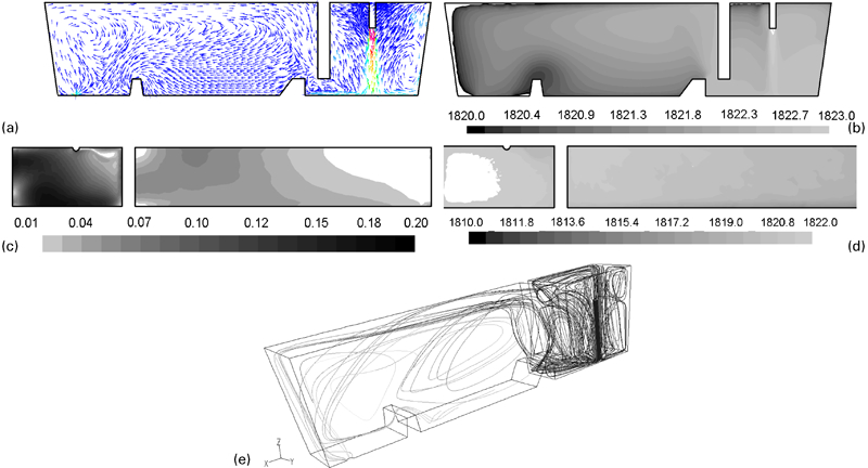
Base case analysis
Temperature contours are analysed at the symmetry plane (Fig. 4b ) and top surface (Fig. 4d ). For all the cases, the range of TCs has been kept constant from 1820 to 1823 K at the symmetry plane and from 1810 to 1822 K at the top surface. This makes it easier to visualise the white area below 1820 K as a cold spot at the symmetry plane. The top surface should be uniformly heated with undercurrents to avoid the formation of any thermally activated vortex, which may come into action when colder liquid lies over hotter liquid. This situation may arise at the top surface near the outlet. Variations at the top surface temperature are monitored and compared to have a full picture of the temperature distribution in the tundish. An average temperature drop of 2·3°C was found from the inlet and outlet streams due to heat loss from tundish walls and the top fluid surface.
The RTD results show a DV percentage of 9, PV percentage of 22 and MV percentage of 69 for prevailing average plant conditions. This corresponds to an MRT of 116 s and an ART of 616 s. The minimum temperature inside the tundish T cold spot was 1810 K, while the maximum surface velocity near the outlet was 0·06 m s−1. This base case reflects a very good overall tundish performance. Thus, an optimal furniture set targets to achieve similar performance with lesser or alternate furniture that is more readily and economically available and provides ease of maintenance.
It would be interesting to assess the contribution from the base case furniture parts that contribute to its performance. The first dam–weir set operates in tandem to guide the flow upwards as fluid moves from the first pseudochamber towards the outlet through the rest of the tundish. The dam at the end of the tundish near the outlet provides an opportunity to avoid a direct flow into the outlet along the bottom of the tundish by directing the flow towards the top again. The absence of this dam would also marginally reduce the surface velocity. Simulation results without this dam suggest that the absence of this dam would introduce lateral streams along the bottom towards the outlet that may destabilise the outlet stream from the tundish. Usage of weir is good from the point of view of tundish metallurgical performance but is perceived as a high maintenance item. Steelmakers are happier to have tundish performance of similar nature without the weir! However, removing the weir from present set costs too much on tundish performance, as can be seen in Fig. 5. In this case, one dam from the base case near the inlet was simulated. The analysis showed that this case deteriorated the tundish performance severely in comparison to the base case. The recirculation (Fig. 5a and e ) was almost absent, and most of the fluid headed directly to the outlet. This was reflected by RTD parameters (Fig. 5f ) as well. The dead volume increased to 13, and PV reduced drastically to 13, whereas the mean MRT reduced by almost half to 61. As can seen in Fig. 5b , the cold zone (white area) also increased, but the cold spot temperature (Fig. 5d ) remained almost constant at 1811 K. The maximum surface velocity near the outlet (Fig. 5c ) also went up sharply up to 0·11 m s−1, which may increase slag entrapment.
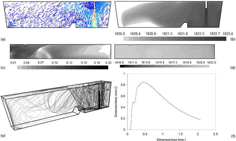
One dam case analysis
Case 2: single higher dam
The dam height was increased from 200 mm originally to 400 mm with a distance of 400 mm from the shroud centre. A higher dam helped to reinduce the circulation (Fig. 6a and e ), but it was not touching the top surface. The flow was reporting to the outlet via the top surface, which was in a way short circuiting. Such a circulation, though increased PV back to 22, further increased DV up to 16 (Fig. 6f ). Things were relatively constant on the temperature distribution front (Fig. 6b and d ). Since a higher dam guided flow upwards, the maximum surface velocity (Fig. 6c ) went up further up to 0·17 m s−1.
One higher dam case analysis
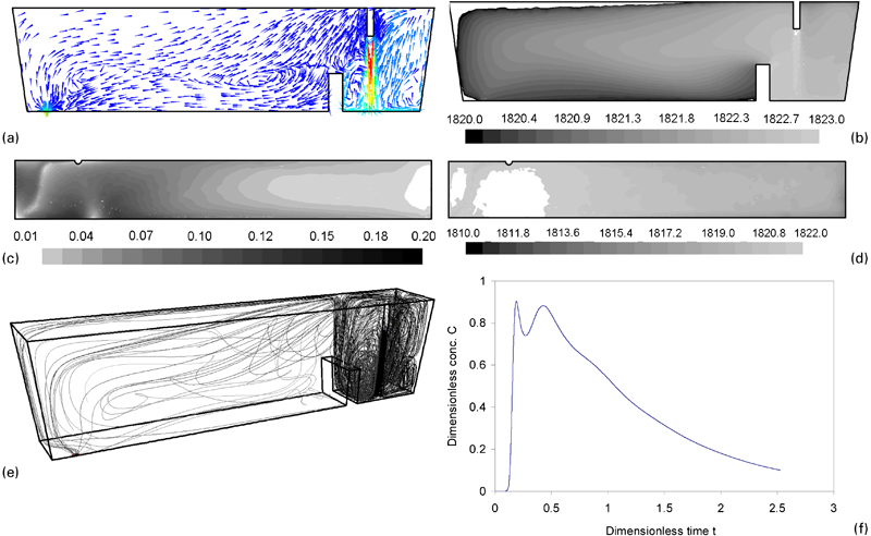
Case 3: Tundish with turbulence inhibitor
Turbulence inhibitors have been used for multistrand tundishes with good results.20 These are easy to put up and maintain and are economical. To have a comparison with the base case, simulation was performed using a typical turbulence inhibitor for the tundish. The simulation results indicated the furniture performance approaching that of the base case. The flow characteristics showed that a large circulation forms as in the base case through the top surface (Fig. 7b and f ). In this case, PV went up to 30% but at a cost of DV that also increased to 14%. The cold zone area was increased with a maximum cold spot temperature of 1809 K (Fig. 7c ). This is reflected in the TC of the surface (Fig. 7e ). Although the maximum surface velocity was on the higher side at 0·1 m s−1, it reduces as it approached the outlet (Fig. 7d ). The RTD curve (Fig. 7g ) reveals an interesting absence of short circuiting flow, as indicated by a single peak.
Turbulence inhibitor case analysis
Case 4: tundish with baffle
A typical optimised baffle design, as shown in Fig. 8a , was analysed. In this case, the baffle was designed to have three rows of holes having different inclination angles as 30, 10, and 0° from bottom to top. The diameter was kept at the maximum possible at 140 mm, and holes were uniformly placed, four in each row. The idea was to have a surface directed flow with circulation as in the base case. Both objectives were met, but even then a small circulation near the top surface just after baffle and channelised flow through top surface to outlet (Fig. 8b and f ) contributed significantly to the dead volume, which went up sharply to 21 (Fig. 8f ). For the same reason, the temperature gradient across the tundish is sharp, as depicted in Fig. 8c , although the top surface is quieter in this case as all the surface turbulence is restricted by the baffle that extends up to the top. The RTD curve in Fig. 8g shows the absence of dual peak, i.e. short circuiting.
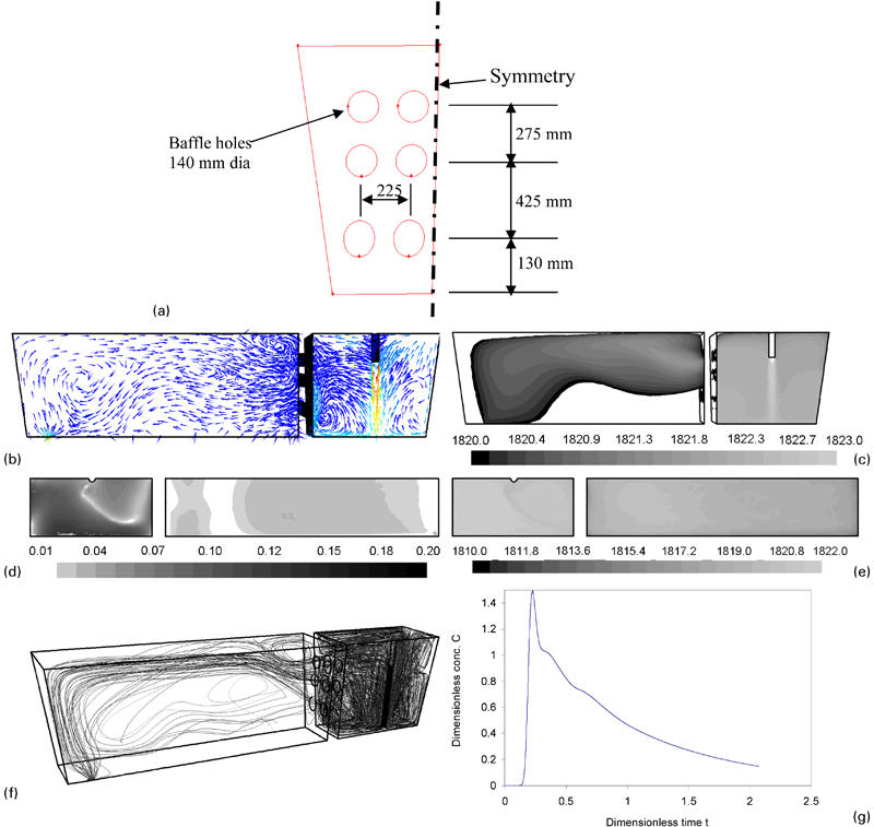
Baffle case analysis
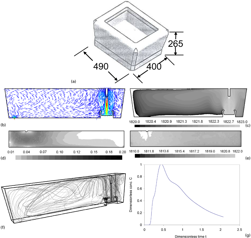
Case 5: tundish with turbulence inhibitor and dam
All the cases in comparison with the base case fail to control the DV, an important quality parameter that cannot be overlooked in a bid for optimal tundish furniture. Although the turbulence inhibitor promises a better plug volume fraction, it increases the DV and reduces the ART. This is probably due to the inability of the turbulence inhibitor to control the flow in the region near the outlet of the tundish. This forces us to go for another piece of furniture that controls flow near the outlet. A simple dam as in the base case has been used in this case along with the turbulence inhibitor. This furniture set-up was found to be at par or even marginally better with the base case. The desired fluid flow characteristics like bulk circulation through the top surface, surface directed flow, etc. were observed in this case (Fig. 9a and e ). This was reflected in the RTD analysis (Fig. 9f ) as well. The PV went up to 36%, while the DV was reduced to 8%, an improvement over the base case. The MRT and ART were observed close to that of the base case. Although the maximum surface velocity was higher than that of the base case, it was within the safe limit near the outlet (Fig. 9c ). The temperature distribution was better than that of the base case as the cold spot temperature was 1814 K (Fig. 9b and d ). This indicates a more uniform temperature distribution in the tundish. Thus, this furniture set-up is found to be an optimal choice for the single strand tundish.
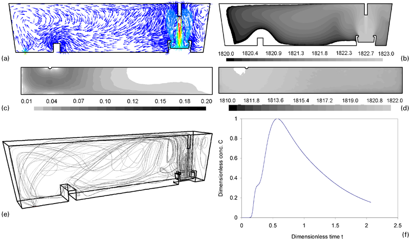
Turbulence inhibitor dam case analysis
A summary of all cases depicting the performance of various sets of furniture used in the simulation is presented in Table 2.
Summary of analysis for various sets of furniture
Conclusions
Various combinations of furniture sets have been compared for a single strand tundish using three-dimensional mathematical modelling with thermal effects. The performance of each set of furniture has been assessed by RTD, velocity and temperature distribution. The buoyancy effect caused by heat loss from the tundish is pronounced and important in assessing the performance of the tundish. This results in a liquid steel temperature drop of 2·3°C as it exits from the tundish. Tundish performance through desired flow characteristics can be achieved by a suitable and optimal use of a set of furniture. Such flow characteristics like circulation patterns, surface directed flow and quieter top surface have been recognised through analysis of the base case furniture. With the help of a comparable analysis, an optimal set of furniture was designed.