Numerical analysis of unsteady hydrodynamics and thermal transport in five-strand asymmetric tundish

List of symbols

Introduction

The tundish in a continuous casting operation is an important link between the ladle (a batch vessel) and the casting mould (a continuous operation). Traditionally, it has served as a reservoir and distributor of molten steel, but now its role has considerably expanded to optimise temperature homogeneity and steel cleanliness. These issues are highly dependent upon the fluid flow and degree of turbulence in the tundish. The state of fluid motion in a tundish significantly influences the rate of heat and mass transfer controlled processes. Most of the metallurgical operations are governed by the nature of the fluid flow, such as spatial velocity distribution and turbulent kinetic energy, and influence the tundish performance considerably, and over decades, a substantial body of work has been devoted to understanding the complex fluid flow inside the tundish.1 ^– 5

Furthermore, several studies have been accomplished to understand the heat transfer phenomenon under different liquid steel flow conditions. The liquid steel jet coming from the ladle shroud produces high turbulence, causing oxygen and nitrogen pickup from the surrounding air, wear of the tundish lining near the liquid jet and slag entrapment from the upper surface into the bulk of the liquid. Steel in the holding ladle looses heat during casting from the ladle walls and upper surface of the bath to the surroundings. Another important aspect affecting the fluid flow phenomena in the tundish is the situation where liquid steel is under non-isothermal conditions. That transforms the flow field into a natural convection situation, which arises because of the strong dependence of the density of liquid steel with temperature.

A number of papers on flow and heat transfer phenomenon are reported. Under steady state conditions, fluid flow and heat transfer phenomenon were mathematically modelled by He and Sahai,6 Szekely and Ilegbusi7 and Joo et al.,8 but in actual casting, the fluid flow and heat transfer phenomena in tundishes vary, particularly during ladle change. Chakraborty and Sahai9 reported the transient fluid flow and thermal fields existing in the tundish. They analysed the effect of transient flow mechanism on the flotation and removal of non-metallic inclusions in the melt.

Lopez-Ramirez et al. 10 investigated the effects of buoyancy forces and flow control devices on fluid flow and heat transfer phenomena in a tundish. They showed that flotation forces affect the fluid flow patterns of liquid steel under non-isothermal conditions. Few studies investigated the aspect of refractory wall wear, which limits the sequence life of the tundish.11, 12

In all of the above, symmetric tundish geometry was used with a single operating strand. There are some studies available13, 14 where multiple strand tundish geometries were used, but in all such cases, the tundish was equipped with an even number of strands. In general, tundish geometry for most industrial practices has centreline symmetry with respect to the impact pad location. There are few cases of asymmetry. To the best of the author’s knowledge, no literature is available for the case of an asymmetric tundish with an odd number of strands. These configurations lead to several issues during casting, such as non-isothermal and transient phenomenon in the flow domain. This non-isothermal nature of the process yields buoyancy forces in liquid steel, which may radically change the fluid flow and have other consequences, such as turbulence intensity, lining wear, surface rippling, gas pickup, intensify slag entrapment and flotation of non-metallic inclusions.

The present investigation aims to numerically simulate the flow and heat transfer phenomena in a five-strand asymmetric tundish. This was accomplished by devising a three-dimensional computational fluid dynamics model with suitable boundary conditions. Starting from basic fluid flow and heat transfer simulations, refractory heating, conjugate heat transfer (CHT) and filling simulations with a volume of fluid (VoF) approach were simulated to meet the requirement of extracting the complex flow and heat transfer physics of the tundish. Such numerical techniques have been applied successfully in several industrial and academic problems.

Geometric description of tundish

The five-strand tundish is equipped with an impact pad located at the bottom of the inlet shroud that is immersed in the liquid metal. Pouring liquid steel in the tundish through submerged shroud produces high turbulence intensity around the pouring point. To circumvent this, the tundish inner bottom wall is mounted with an impact pad placed below the ladle pouring point.

The inlets of the strands are mounted with cylindrical extruded parts with the objective of increased residence time of the liquid metal before entering the moulds. These break away and float in the slag during the course of casting operations. The geometrical dimensions and the operating parameters are presented in Table 1.

Model formulation

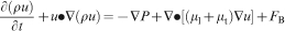
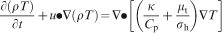
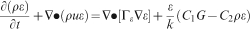
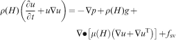
The mathematical model is based on the assumptions of continuum hypotheses that demand the mean free path within the permissible limits. Fluid is assumed to be incompressible, Newtonian and to follow Boussinesq’s approximation in density variation. The turbulence kinetic energy and intensity are assumed to be in equilibrium with the fluid flow and liquid state enthalpy. Considering those approximations, the governing equation consists of the simultaneous solution of continuity, momentum transfer and energy transfer equations under turbulent unsteady conditions together with the equations of turbulent kinetic energy k and its dissipation rate ϵ:

Mass (1) Momentum (2) Energy (3) In these equations, F _B is the buoyancy force term, u is the time averaged velocity vector and T is the steel temperature in the three-dimensional (3D) domain. Additionally, μ _l and μ _t are the molecular and turbulent viscosities of steel respectively, and κ is the steel conductivity. The turbulent viscosity is calculated by knowing the turbulent kinetic energy and its dissipation rate, which are given by their conservation equations.

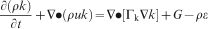
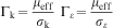
Kinetic energy (4) Dissipation rate (5) and (6) where Γ _k and Γ _ϵ are the diffusion coefficients for the turbulent kinetic energy and its dissipation rate respectively and are given by (7) where μ _eff is the effective viscosity and is given by μ _eff = μ _l+μ _t.

The tensor expression for the generation term G is given as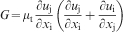 (8) The values for C_μ , C ₁, C ₂, σ _k, σ _h and σ_ϵ are 0·09, 1·44, 1·92, 1·0, 0·9 and 1·3 respectively.

Initial and boundary conditions

In the present investigation, suitable boundary conditions for flow and temperature were incorporated, as used in the published literature.10 ^– 15 At the shroud exit, the mean velocity was assumed to be uniform though its cross-section, and the other two perpendicular velocities were assumed to be zero. The turbulent kinetic energy and its dissipation rate were assumed to be uniform and calculated in terms of a fixed value of turbulence intensity at 6%. Boundary conditions for momentum transfer at all solid surfaces, including walls and bottom of the tundish, walls of cylindrical extruded tubes, surfaces of impact pad, were those of non-slipping. Zero normal gradients were imposed at symmetry planes and frictionless conditions at the free surface of liquid steel. Similar boundary conditions were established for turbulent kinetic energy and its dissipation rate. Near any solid surface, the logarithmic law for velocity distribution was applied.16 At outlets, a pressure boundary condition was adopted.

Regarding the heat transfer equation, the boundary conditions include heat losses through the wall, bottom and free surface of fluid in the tundish. Assuming a slag thickness of 35 mm, heat flux conditions were obtained from the previous literature.17 The boundary conditions of these fluxes are 1·4 kW m⁻² from the bottom, 3·2 kW m⁻² from the vertical–longitudinal walls, 3·8 kW m⁻² from the transverse–vertical walls and 18 kW m⁻² from top free surface. The heat flux conditions used in the present investigation are well established and were used in most of the numerical studies.5,10 ^– 15 The heat flux conditions for the walls of cylindrical extruded tubes were assumed to be the same as the bottom of the tundish wall.

Mathematical simulations of the process consisted of employing a constant flowrate of incoming steel from the shroud at an initial temperature of 1823 K. For starting the simulations of the unsteady state conditions, the flow and thermal fields under steady state conditions were employed as the initial conditions in the 3-D computational domain.

Numerical solution procedure

Tundish geometry and grid were generated using a software Gambit, while the governing equations were solved using a computational fluid dynamics software Fluent that uses the finite volume technique. The semi implicit method for pressure linked equations algorithm was used to avoid pressure–velocity decoupling. A third order upwind scheme QUICK was used to discretise the convective terms in the momentum and energy equations. To input the physical properties of the fluid, the constant density method was used. To prevent numerical oscillations, the necessary conditions for time stepping were determined from the Courant–Friedrichs–Lewy condition. A grid independence study based on particle residence time was carried out to choose the optimum grid points. Table 2 show the results of the grid independence study based on average particle residence time, indicating that grid independence was arrived at with 1·5 million cells to be computationally economical. An appropriate grid density scheme was adopted to capture small scales structures and fitting turbulence y⁺ value in a permissible range. The density and dynamic viscosity of the molten steel was taken as 7000 kg m⁻³ and 0·00648 kg m⁻¹ s⁻¹ respectively.

Model validation

The mathematical model was validated with the experimental data of a single strand tundish.18 For doing such validation, it is necessary to generate tundish geometry as per the reported geometrical dimensions. Therefore, as reported,18 the experimental data of dimensionless concentration were chosen for a tundish having W/L ratio of 0·215. The calculated dimensionless concentration data of the present mathematical model were compared with the experimental data reported in the literature18 and found to be in good match. This is shown in Fig. 1.

OPEN IN VIEWER

Figure 1.

Comparison of experimental and predicted concentration curves

Results and discussion

Numerical experimentations were performed for the tundish for various situations. Invoking plant operating practices, simulations were carried out to mimic the actual plant process situations.

Following are the numerical experimentations carried out:

It should be noted that for all the cases, simulations were performed for both steady and unsteady states. For the steady state, iteration loops were continued until global error reached a limiting value, i.e. <10⁻⁴, whereas for unsteady state simulations, these were performed until the system reached a dynamic steady state. The inlet melt temperature corresponded to the last temperature of the ladle outlet stream of the previous heat in a sequence casting operation. Using the calculated flow and thermal fields as the initial guesses, unsteady state calculations were carried out over the initial few heats of the casting period.

To capture the exact physics of the problem, it is necessary to invoke the actual plant operating conditions during numerical simulations; however, it is always not possible to put the exact numerical values of the plant conditions in the simulation case. In such situation, it is necessary to convert those conditions to one suitable for simulation case sets. Table 3 shows the typical operating conditions of the tundish at the plant. Table 4 represents the converted boundary conditions used in the simulation case sets.

Steady state fluid flow simulation

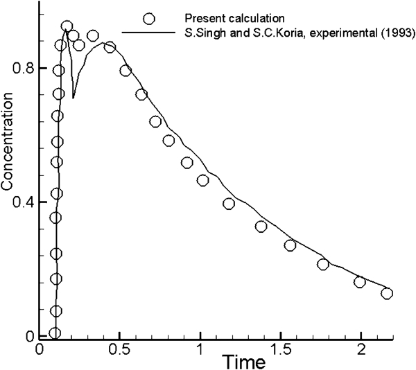
The displays of velocity and temperature presented in the following discussion correspond to a–vertical plane passing through the outlets. The velocity vector field under the steady state condition at a plane passing through the outlets with steel at 1823 K is shown in Fig. 2a . Note that the magnitude of the plotted velocity vectors and the subsequent velocity plots are proportional to their lengths. To capture the exact flow field away from the ladle stream, a few massless particles were injected from the inlets, and their trajectories were tracked over time. Figure 2b shows the trajectory of these particles in terms of the time taken by the particles to reach the outlets.

OPEN IN VIEWER

Figure 2.

a velocity vectors of liquid steel at plane passing through outlets under steady state flow simulation and b particle tracks under steady state flow simulation

It is seen that there is a formation of slow moving zone at the farthest strands. The formation of a complex velocity field with recirculating flows throughout the whole zone is also observed. Figure 2b shows that the massless particles take longest to reach the farthest strands, and there is a strong recirculatory flow with high velocities near the free surface and a steady distribution of the liquid metal at the strand exit.

Steady state fluid flow coupled with heat transfer simulation (considering buoyancy effect)

The steady energy equation was solved for calculating the temperature field in the tundish. Figure 3 shows the temperature contours at a plane passing through the strand outlets. The temperature in the plane of the entering liquid jet was found to be almost homogeneous and was probably due to the heavy mixing promoted by the turbulent flow; however, downstream, thermal stratification was readily observed. There was a uniform distribution of temperature contours inside the tundish, with no significant temperature differences between the liquid streams found at the strand exits. High temperature gradients were formed near the free surface of the liquid owing to the high heat flux of the surroundings. Average heat losses were calculated at the tundish walls and found to be of nearly uniform distribution.

OPEN IN VIEWER

Figure 3.

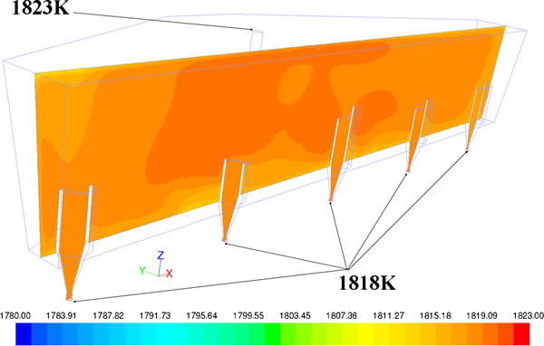
Contours of temperatures at plane passing through outlets under steady state fluid flow coupled with heat transfer simulation

Steady state heat transfer simulations for different liquid metal heights

The basic aim of this study was to determine the transient effects during filling operations, and simulations were performed with several liquid metal heights to mimic the filling of liquid metal in the tundish. Three liquid metal heights were considered, i.e. 430, 500 and 700 mm.

Figure 4 shows the temperature contours on a plane passing through the strand exits. It can be seen that there was a uniform distribution of temperature gradients inside the tundish, and thermal stratification was found to decrease with the increase in liquid metal depth.

OPEN IN VIEWER

Figure 4.

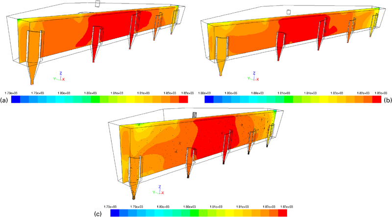
Contours of temperatures at liquid steel height of a 430 mm, b 500 mm and c 700 mm

Global temperature drops were calculated at the strand exits by defining a heat loss parameter that will determine the maximum temperature drop with increasing/decreasing depth.

Mathematically, the temperature drop Δθ was defined as (9) where T is the temperature, and T _inlet = 1823 K

Table 5 shows the temperature drops for different liquid metal depths.

OPEN IN VIEWER

Table 5.

Temperature drops at strand exits (K)

Liquid metal height	Strand#1	Strand#2	Strand#3	Strand#4	Strand#5
430 mm	5	1	1	3	7
500 mm	4	1	1	3	7
700 mm	5	2	1	3	8

It can be seen that the maximum temperature drop was at strand 5, whereas strands 2 and 3 have similar values. The maximum temperature drop increased with the increase in liquid metal depth as an increase in liquid volume causes an increase in surface area and therefore enhanced heat transfer rate.

Transient heat transfer simulations for different strand opening schedules

A general practice for multistrand tundish is that the strands are opened in a specific sequence that is plant specific. In order to understand the thermo fluidic effect during strand opening and the thermal stratification, simulations were carried out as per the plant practice; 4–2–5–1–3. The total strand opening time was ∼3 min.

Based on these data, simulations were performed for the strand opening schedules by opening the fourth strand first and keeping the others closed; then, transient stepping was carried out for 45 s. During the second run, using the initial conditions from the preceding step (i.e. initial fields for the flow and temperature from the first step), strands 4 and 2 were opened while the other strands were kept closed. Then, simulation was performed again for 45 s and so on. In this way at the final run, transient computations were carried out for 45 s by opening all the strands. The total duration of transient computations was up to 3 min.

Figure 5a–d shows the temperature contours for different strand opening schedules on a plane passing through the strand outlets. It was observed from those figures that there were no significant differences in temperature at the strand exits. Temperature contours typically showed steady distribution with uniform temperature gradients. Temperature drop was found maximum at the first run and became nearly identical at the end.

OPEN IN VIEWER

Figure 5.

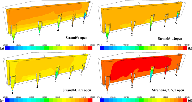
Contours of temperatures for different strand opening

Table 6 shows the temperatures at different strand exits for different strand openings. It was evident that the strand outlet temperature was lowest at the first run, and it became almost same at the final stage. Maximum temperature drops at the strand exit to an inlet temperature of 1823 K were found to be only 5 K.

OPEN IN VIEWER

Table 6.

Temperatures at different strand exits for different strand openings (K)

Sequence no	Strand#1	Strand#2	Strand#3	Strand#4	Strand#5
Open #4				1805
Open #4, #2		1805		1807
Open #4, #2, #5		1807		1807	1805
Open #4, #2, #5, #1	1818	1818		1819	1817
Open all strands	1818	1818	1819	1819	1818

Refractory heating simulations

The heat transfer simulations carried out earlier were based on the heat flux boundary conditions from the literature.17 This allowed us to come to a conclusion that the heat flux boundary conditions may not be perfect, and further modification was required for better heat transfer prediction. Those modifications can only be incorporated if exact refractory preheating simulations are performed so simulations were performed for refractory heating to evaluate the temperature profile at the refractory linings. The basic purpose of doing this was to couple the fluid simulation with refractory temperatures, i.e. replacing the heat flux boundary conditions with exact heating conditions of tundish preheating.

Using measured plant tundish, three layers of refractory shell linings were considered. The thicknesses of inner refractory bricks, safety lining and outer steel casing were 125, 113 and 26 mm respectively. The total refractory heating time was 240 min.

For such simulations, it was necessary to know the convective heat transfer coefficient from the refractory and steel casing. This was modelled as refractory with forced convective conditions and steel with natural convective heat transfer conditions. Those values exactly reflect the conditions at plant. The final refractory heating temperature at plant was limited to 1573 K. Such heat transfer coefficients were calculated from the literature and are given by the following equations.

Natural convection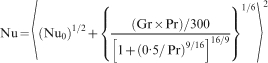 (10) where Nu is the Nusselt number on the wall and given by Here, h is the convective heat transfer coefficient per unit area, L is the characteristics length and k is the thermal conductivity respectively. Gr, Pr and Nu are the Grashoff number, Prandtl number and Nusselt number calculated at the free stream conditions.

Forced convection:

Here, Dittus–Boelter correlations have been used as (11) where Re is the Reynolds number based on bath height.

After calculation from the correlations (equations (10) and (11)), the numerical values of forced convective heat transfer coefficient at the inner refractory lining and natural convective heat transfer coefficient at the outer steel casing were obtained as 60 and 8·234 W m⁻² K⁻¹ respectively.

Considering the above geometrical and boundary conditions, a refractory mesh was generated for starting up the simulations. The number of tetrahedral cells used was 0·5 million.

Figure 6a shows the temperature contours after tundish preheating and Fig. 6b the temperature contours at different planes in the refractory after preheating. The typical distribution shows the highest thermal gradient at the working lining, and it has minimum value at the steel wall. There is a lateral spread of the temperature contours at the bottom of the working lining. This implies localised heating with a high rate of heat transfer from the surfaces.

OPEN IN VIEWER

Figure 6.

Contours of temperatures a after tundish preheating and b at different cross-sections

With the preheated refractory from refractory heating simulations, fluid flow results were coupled for starting up transient heat transfer simulations. Boundary conditions for heat flux were modified with the exact refractory heating data. Transient thermal energy equation was solved for ∼200 s after reaching the dynamic steady state condition. It was found that there was no such non-uniformity in temperature distribution. The maximum temperature drop was found to be 6 K.

Transient filling simulations with VoF method

The objective of this study is to find the transient dynamics and heat transport phenomena when liquid metal is poured into the empty tundish. Imitating such a situation demands the solution of mass, momentum, energy and volume fraction equations at each time instant during filling. This is inherently time consuming and requires several hours to compute. A complex geometry like the present tundish with 1·5 million cells will take ∼2 months to give final results. Having such limitations, simulations have been carried out for a smaller height of 430 mm. For the present case of 180 s of simulation time, it took ∼45 days for the final results.

Volume of fluid method

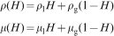
In this method, the governing equations (equations (1)–(3)) were modified in terms of void fraction for both phases. A void fraction F was defined as the fraction of liquid inside a control volume (cell), with the void fraction taking the values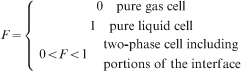 (12) Based on the void fraction, the governing equations were modified as (13) (14) where g is the gravitational acceleration, f _sv is the surface tension force and ρ(H) and μ(H) are the density and dynamic viscosities, which are defined by (15) The subscripts l and g denote the quantity with respect to the liquid and gas phase respectively. H is the heavy side function.

Since the fluid type remains constant along particle paths, the void fraction F is passively advected by the equation (16) Filling results

Considering liquid steel as the primary fluid and air as the secondary fluid, simulations were performed for ∼200 s with time step size as 10⁻⁶.

At t = 0, liquid metal starts falling in the tundish from the inlet, and as time advances, it fills up. Figure 7a–e shows isocontours of void fractions of the liquid steel for different time instants. Here, it can be seen that at about t≈80 s, the liquid metal reaches all the strand exits.

OPEN IN VIEWER

Figure 7.

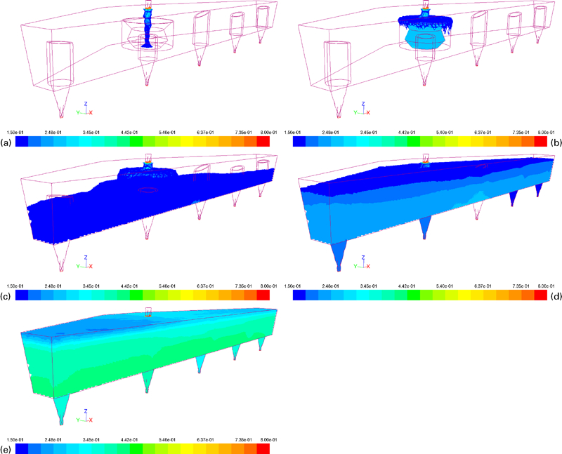
Void fractions of liquid steel for different time instants

From the simulation, the filling time was found to be 160 s, whereas the actual filling time at the plant was about 180–190 s. This supports the validity of our result. A quantitative result of temperature values at the strand exits has been calculated for t = 80 s. It was found that the maximum temperature drop from the inlet and outlet was 6 K.

Transient simulations with unheated refractory

The basis of this analysis was to predict the importance of proper tundish preheating practice. The effect of inadequate preheating was brought about by setting the simulation conditions of non-preheated tundish (room temperature). The tundish was in operation at a lower liquid metal height of 430 mm, and the full refractory insulation domain was considered. Such a situation demands CHT study, where heat dissipation was due to the coupling of convection and conduction. Radiation effect was also considered with convection.

The mode of conduction and convection in CHT was coupled by intermedium flux balance, i.e. the convective flux was balanced by conduction and radiation flux. Considering such methodology, the boundary conditions were modified as follows.

Outer steel casing:

Total heat transfer coefficient = h = h _convective+h _radiative = 14·234 W m⁻² K⁻¹

Refractory:

Initial temperature of refractory, safety lining and outer steel casing = 303 K

Inlet temperature of liquid steel = 1823 K

Bare refractory walls = h _radiative

Considering liquid steel at 1823 K, transient simulations were performed by patching insulating walls at room temperature. Transient simulations were carried out for ∼400 s, and strand outlet temperatures were monitored at different time instants.

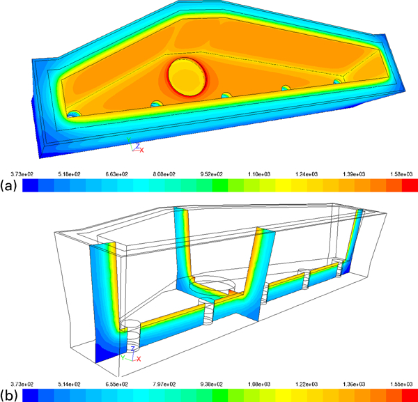
Figure 8a shows the velocity vectors at a plane passing though the strand. As before, there was the presence of recirculatory zone. Figure 8b shows the contours of temperature of the liquid steel at a plane passing through the strands. This result was at t = 180 s.

OPEN IN VIEWER

Figure 8.

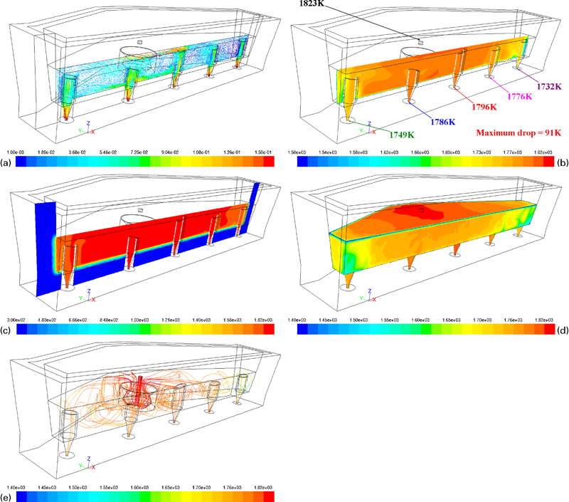
a velocity vectors at plane passing though strand, b contours of temperature of liquid steel on plane passing through strands, c temperature contours coupled with refractory insulation at plane passing through strands, d contours of temperatures of liquid steel at different planes and e particle tracking simulation results in terms of temperature values

A typical observation made from this contour was that there was a huge temperature drop at the strands, and the maximum temperature drop was ∼91 K. The outlet temperatures of each strand are shown in Fig. 8b . This clearly shows that at strands 1 and 5, liquid steel reaches its freezing temperature. There was an abrupt change in temperature gradient at the locations nearer to these strands. Such an abrupt change in the gradients causes enhancement in heat transfer and thereby reaching liquid steel freezing temperature. Figure 8c shows the temperature contours coupled with the refractory insulation at a plane passing through the strands. It is evident that walls at the CHT zone form a localised change in temperature gradients, which affects conduction of heat through the walls. Figure 8d shows the contours of temperatures of liquid steel at different planes. These 3D temperature contours in different 2D planes clearly indicate a sudden drop in temperature values at the corners. These temperature drops are the limited values of freezing temperatures at the corner locations and show that the probability of freezing of metal was high at strands 1 and 5. Figure 8e shows the particle tracking simulation results in terms of temperature values. This result shows a continuous drop in liquid stream temperature as it approaches the strand exits. This drop was maximum for strands 1 and 5.

Conclusions

Starting with the steady state fluid simulations, several heat transfer simulations for different operating conditions were performed.