Preliminary investigation of influence of temperature on decarburisation using fundamental AOD model

Abstract

A high temperature thermodynamics model was earlier coupled with a fundamental mathematical model describing the fluid flow in an argon–oxygen decarburisation (AOD) converter and was initially validated for an idealised temperature description. More specifically, a linear average temperature relation was used such that the temperature would be isolated from other effects such as reactions and mixing. Thereafter, the effect of the starting temperature on the decarburisation was studied. The purpose is to provide some initial knowledge about how temperature affects the decarburisation in an AOD converter. The results suggest that the thermodynamic limit for carbon concentration after reaching the carbon removal efficiency (CRE) maxima is vertically translated downwards at higher temperatures. Furthermore, when plotting the mass ratio between CO and CO₂, there is an indication of a point that may relate to a CRE maximum.

Introduction

The argon–oxygen decarburisation (AOD) converter is a common reactor for refining of stainless steel grades. The process has a high productivity and yields a good reduction of carbon and sulphur with small chromium losses. The AOD converters’ main tasks are to reduce the carbon and sulphur concentrations and to increase the temperature. The temperature increase originates from the reaction heat of the oxidation of alloying elements, primarily silicon, carbon, manganese and chromium. The consequence is an unwanted decrease in chromium and manganese contents in the steel since they counteract the certification of the steel grade analysis.

Fruehan investigated the influence of a temperature increase1 on decarburisation for incremental levels of decarburisations. He concluded that the changes did not differ to any significant degree and suggested that an average process temperature of 1675°C could be used when calculating the decarburisation. In 1978, DebRoy and Robertson developed a model2 in which they calculated the compositions at different depths in the melt. Later, they calculated the refining of the whole converter and compared the prediction against heat data3 and found a fairly good agreement. Their approach was to use a heat balance to describe the temperature.

Previously, Wei and Zhu developed a mathematical AOD reaction model4 for a side blown converter and used a heat balance to account for the temperature increase. Later, they made a preliminary investigation of a reaction model5 for a combined top and side blown converter and concluded that the temperature approach used in the side blown converter was not appropriate for the combined top and side blown converter. They expanded the heat description6 by solving the energy equation for a two-dimensional (2D) geometry and pointed out that factors such as an initial temperature can, to different degrees, directly influence the decarburisation rate. In 2011, Järvinen et al. 7 and Pisilä et al. 8 presented a model that simulated the temperature in the liquid steel at each time step. The method seems similar to DebRoy and Robertson’s as well as Wei and Zhu’s earlier methods.4

Previously, a fluid flow model9 was developed and later augmented with chemical reactions10 and was used in this study to investigate the effect of the starting temperature on the decarburisation during the first injection step. However, in the present study, a regression from TimeAOD211 data was used to describe the temperature in the converter and is a further development of the Sjöberg dynamic model,12 where parameters are adjusted to fit the samples taken from the process in order to calibrate the model and provide a valid calibration window. The model considers gas, steel and slag in a single reaction cell and computes temperature and composition of steel and slag. Furthermore, the temperature is calculated via total heat balance before and after the composition has been calculated; thus, the energy required for heating up the gas and the slag is considered together with the reaction heat and losses due to convection and radiation.

The part of the decarburisation period that has been studied in the current research is defined in Fig. 1. The present model was verified for an industrial heat assuming an ideal dissolution of additions. Thereafter, a parameter study was made for different starting temperatures to see the effect on the rendered decarburisation rates. This kind of parameter study has not previously been reported in the open literature.

Figure 1.

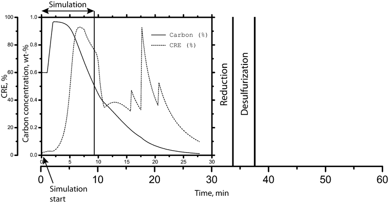
Schematic view of what is simulated in process

Model description

The computational domain can be seen in Fig. 2, where the tuyeres are located at the bottom left of the converter. Schematically, the greyish contour shows the gas distribution in the converter. The arrows show the main flow of the steel and are intended to give a schematic description of the motion in the converter. The gas is injected at the bottom left side. A part of the gas is pushed forward parallel to the bottom, which results in the vortex seen in the tuyere area. Another part of the gas is more or less immediately drawn upwards due to buoyancy forces, which cause the steel to make another vortex in the x–z plane. These vortices meet in the middle right part of the figure, which distorts the vortices and brings back the steel to the tuyere side of the converter. Moreover, the clockwise vortex pushes the counterclockwise vortex into the back of the converter, also creating a vortex in the x–y plane. An in depth analysis of the reactions and flow was earlier reported by the authors.13

Figure 2.

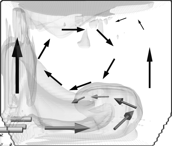
Schematic view of main steel flow and gas hold-up in converter model

Fluid flow model

The mathematical model of gas injection in an AOD converter is 3D and accounts for the steel, gas and slag phases (three-phase). The PHOENICS software,14 which was used to solve the model equations, is used to solve two separate sets of Navier–Stokes equations. One set for liquid phases and one for the gas phase, using the IPSA algorithm.15 Moreover, the present AOD model is based on an earlier model16 to which new transport equations and new auxiliary equations have been added and/or modified, since the fluid slag is incorporated. Further, the model is augmented to account for bubble swarms.

The fluid flow model is based on the following assumptions:

the AOD converter is calculated using only a half 3D grid due to symmetry along the middle plane; the domain contains 50 t steel (a half size converter)

ii.

the free surface is flat; the gas bubbles are allowed to leave the domain through the surface

iii.

the gas bubbles are introduced through three nozzles located in the side of the wall; the gas flowrate through nozzles 1, 2 and 3 is 20 Nm³ min⁻¹ respectively

iv.

the injected gas adopts the steel temperature momentarily; however, the cooling effect on the steel is considered in the TimeAOD2 data11

an interface friction coefficient is used to describe the force between the gas phase and the liquid phases, i.e. to couple the two separate sets of Navier–Stokes equations

vi.

the energy equation is not solved for; therefore, the liquid and gas temperatures are set to time dependent functions (increases linearly with elapsed time according to a regression of TimeAOD2 data11 for the industrial heat under consideration)

vii.

the liquid slag phase is homogenous and treated as liquid spherical droplets; in addition, it is initially supposed to cover the steel by a 6·3 cm thick layer on top of the steel phase

viii.

the solid part of the slag is not transportable; however, it contributes to a higher metallostatic pressure.

Transport equations

General equations

Based on the assumptions above, the following equations are solved in the 3D three-phase fluid flow model of gas injection in the AOD converter:

mass conservation equations for the steel, gas and slag phases

ii.

equations for conservation of momentum in the x, y and z directions for the steel, the liquid slag and the gas phase.

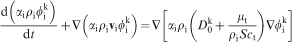
The flow field was obtained from previous simulations by solving the equations in the 3D three-phase fluid flow model of gas injection in the AOD converter.9 In addition, the following transport equation is used for transport of any species, of phase i (1) where α _i is the phase volume fraction, ρ _i is the phase density, t is the time, v _i is the phase velocity vector, is the diffusion coefficient for specie k, μ _t is the turbulent dynamic viscosity and Sc _t is the turbulent Schmidt number (set to 1).

Slag phase

Incorporation of the slag phase into a three-phase model of a steel bath has earlier been reported.17 ^– 20 Regarding movement of the liquid slag phase within the steel phase, considering a Eulerian method, it is possible to correlate the relative velocity between a slag phase and steel as a function of the flow variables, as shown in references.20 ^– 23 A detailed description of the slag implementation in the model for the flow calculations can be seen in Ref. 9.

Gas phase

The gas phase was treated as a continuous phase. The PHOENICS software solves two separate sets of Navier–Stokes equations, one set for liquid phases and one for the gas phase, using the IPSA algorithm.15 The steel and gas phases are coupled by bubble drag. The gas phase is assumed to follow the ideal gas law, and the bubble size is calculated according to Oeters.24 In the model, the bubble size has a dependence on temperature through both the gas and the steel density.

The ideal gas law has been used to calculate the gas density using temperature and pressure calculated as the static pressure implied by the weight of the mass above plus the pressure from the dynamic head. The metallostatic pressure in a cell is calculated using a mean density value by considering the amount of gas that is located above it. Further terms are added for bubble drag, for bubble swarm drag and for the gas cavity just outside the tuyeres.9 However, the top slag inflicts an additional force on the steel bath that will increase the pressure in the melt. The pressure exerted from the rigid top slag on the bath surface was calculated according to the following equation25 (2) where m is the mass of the rigid top slag, g is the gravitational acceleration and A is the area of the bath surface (assumed smooth). Further details can be found in Refs. 9 and 25.

Reference heats

In Fig. 3 the temperature predicted by TimeAOD2 model is shown together with the linear regression used in this study. The reactions are believed to change locally during the dissolution period, which is not considered in this study. Thus, the first part is assumed to be an ideal dissolution of the additions. Furthermore, the difference between the reference heats can be seen to have different lengths for the first injection step. Moreover, they have quite similar temperature profiles. In TimeAOD2, the first 3 min is set as a slag build-up period, where primarily Si is assumed to oxidise. However, Si is not included in the present model. Therefore, to be able to compare the results, a time translation is necessary. Thus, the predicted data are translated to the first decrease in carbon in the reference heat.

Figure 3.

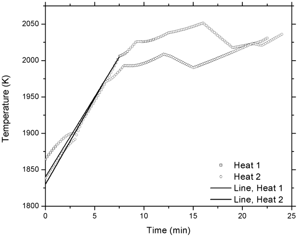
Linear regressions used in simulation compared with TimeAOD2 data

The TimeAOD2 model11 takes temperature into consideration, including heat from reactions as well as cooling effects of gas and slag. Furthermore, in the TimeAOD2 model, the temperature is assumed to be constant for the whole domain. A consequence is that the temperature at the injection point and that at the surface of molten steel are identical. This assumption results in deviations from the real temperature in those regions and may alter the amounts of reaction products. However, the results could still provide a good approximation as have been shown by others,2 ^– 5,26–28 where only a single calculation cell has been considered with satisfactory results. Moreover, it should be noted that with this temperature assumptions, the model will only be consistent for the given analysis and gas flowrate. However, the present model is intended to be further developed to be consistent for a broad range of heats in the future by solving the energy equation.

Earlier, an investigation of the effect of a solid part of the top slag on the decarburisation from a pressure perspective was conducted by the authors.25 The same implementation was used here. However, the top slag was calculated according to the amount of lime added with an estimated Si oxidation from the reference heats. In the earlier study, the typical end slag weights after the whole decarburisation were used; thus, a smaller amount of solid top slag is considered in this study. More specifically, ∼45 kg slag per tonne of steel was used in this study.

Thermodynamics

The Thermo-Calc29 software package is a widely used tool for calculating phase equilibria and phase diagrams. Based on a strong algorithm, the Gibbs energy minimisation method, Thermo-Calc has a wide area of use within thermodynamic analyses. In this study, Thermo-Calc (TQ-interface ver. 7), equipped with the databases TCMSI130 (Themo-Calc Metal Slag Interaction, ver. 3.0) and SSUB431 (SGTE Substance Database, ver. 4.1), was used to predict local equilibrium phase distributions. The database TCMSI1 contains thermodynamic data regarding steelmaking slag equilibrium and metal–slag interactions, whereas the SSUB4 database contains thermodynamic data for many condensed compounds and gaseous species. Even though the databases contain data for many different elements, the complexity of finding a solution is increased for every element added. Thus, a selection of the five most important elements to the refining process was chosen, as carried out in the earlier studies.10, 13, 25 The system was defined with the elements Fe, C, Cr, Ni and O, which could take the form of gas, liquid or one of the following stoichiometric oxides: FeO, Fe₂O₃, Fe₃O₄, Cr₂O₃ and NiO. In addition to these oxides, the model predicts a spinel phase Cr₂FeO₄ to be stable at high pressures and high oxygen activities. However, the formation of this spinel phase is controlled by kinetics. It is therefore hard to calculate the amount that would be expected to form in this model. Therefore, the spinel phase was excluded in order to keep the simplicity of the model.

The transported gas species are in accordance with previous studies:13, 25 O₂, CO and CO₂. The reason why transport of species is preferred to element transport is to distinguish the gas species from each other (O₂, CO and CO₂) in the transport equations.

Coupling

The interface between Thermo-Calc and PHOENICS is a programming interface known as TQ.29 This is an interface within the Thermo-Calc software package that is implementing functions in the native language of Thermo-Calc. This enables a reasonably quick handling of functions for the thermodynamic calculations. The communication between the TimeAOD2 model and the PHOENICS is purely static. Data regression is made externally and statically inserted to the PHOENICS software.

The computational fluid dynamics part of the model computes the convection and diffusion of reaction products and elements. In each horizontal grid plane, if the conditions are met, thermodynamic calculations are made in the plane cell wise. Reactions take place if the gas volume is between 20 and 99·5% in a calculation cell. Equilibriums are calculated at the beginning of each time step and when the gas composition has changed by 5% units or more.

Formulation of coupled problem and method of solution

Using a steady flow field9 scalar transport (equation (1)) was applied to transport the thermodynamic quantities, i.e. the flow field itself did not change during the reactions:

only the initial injection stage is considered, where the injected gas is assumed to be 100%O₂

ii.

thermodynamic equilibrium is assumed to be reached in every cell in each time step

iii.

within each time step, the steel temperature is assumed to be constant within the domain; the domain temperature increases linearly with elapsed time according to regression of TimeAOD2 data11 for the industrial heat under consideration

iv.

the reactions taking place include the following elements: Fe, Cr, Ni, C and O; as mentioned, in the present work the gas description has been improved to transport the gas species O₂, CO and CO₂.

Using the commercial software PHOENICS14 coupled with Thermo-Calc,29 the solution used three 200 number of 0·125 s time steps and took ∼72 h on a standard PC with core i7 at 3·0 GHz.

Fundamentally, the time step needs to be small enough to allow all the injected gas to react before it leaves the bath. If it is, for time averaged, i.e. Reynolds averaged Navier–Stokes approach, minor changes of the size of the time step do not seem to affect the results remarkably. However, solving the energy equation in the future may bring considerable tougher restrictions on the time step for consistent results.

Validation

The two industrial heats chosen to validate the model were taken from an RFCS project,32 in which Outokumpu Stainless AB participated. In this project, batches of heats were sampled at certain points in the process. Furthermore, for the selected heats, the initial additions were considered for the start values of the chemical compositions. However, for the temperature, an ideal dissolution was assumed. The Outokumpu Stainless, Avesta steelworks uses mainly stainless scrap, and the carbon content is thereby quite low, namely between 0·5 and 2·5 wt-%. The only variable that was not available was the dissolved oxygen in the liquid steel. Therefore, an equilibrium calculation was made to determine the saturation value, which was used as input data (Table 1).

Table 1.

Initial conditions used for validation heats and parameter studies

Heat no.	C/%	Ni/%	Cr/%	O/ppm	T/K
1	0·78	7·81	17·73	176·9	1840
2	0·63	8·27	17·65	157·9	1830
3	0·63	8·27	17·65	157·9	1850
4	0·63	8·27	17·65	157·9	1860
5	0·63	8·27	17·65	157·9	1870

Parameter study

The starting temperature of the liquid steel in the AOD process varies typically from 1773 to 1973 K, with the aimed temperature of 1853 K. Furthermore, the temperature is decreased by the additions, e.g. ferro chromium, lime, etc. One of the validated cases was chosen as a reference for the parameter study. From this reference, the start temperature was varied between 1830 and 1870 K.

Results

Validation

The dissolved carbon content in the steel melt compared with the predicted concentration can be seen in Fig. 4. A time translation has been used in order to compare the decrease in the carbon content. For the reference heat, the carbon content is seen to increase during the first 3 min as dissolution of additions begins and the steel melt absorbs carbon. Thereafter, it begins to decrease.

Figure 4.

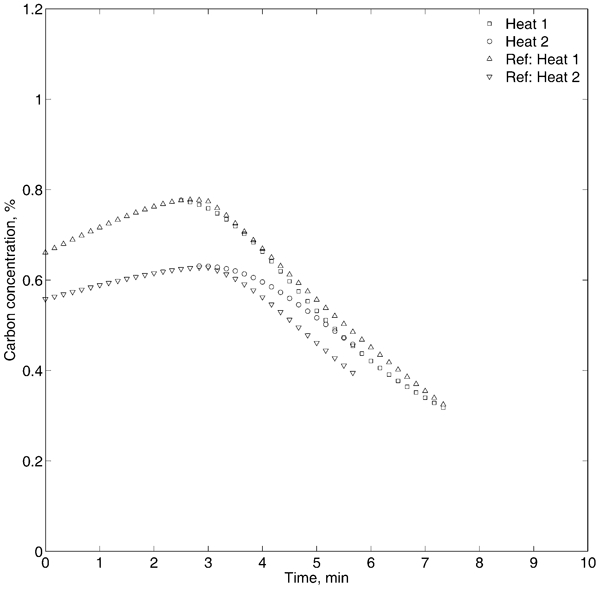
Carbon concentration as mass percentage plotted over time as predicted by model compared with reference heats predicted by TimeAOD2

The carbon concentration was computed as follows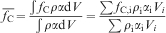 (3) where f _C,i is the carbon fraction in cell i, ρ _i is the density in cell i, α is the phase volume fraction and V _i is the volume of cell i.

In Fig. 5, the corresponding carbon removal efficiency (CRE) can be seen. Here, the increase in the CRE value is matched rather well for both heats, whereas the maximum value differs by as much as 30% units from the reference value. Initially, the CRE value increases slowly for the reference heats during the first 2 min. Thereafter, it increases rapidly to flatten out after reaching the maxima and later decreases slowly. However, the authors’ model predict a higher CRE maxima in the shape of a peak instead of the flatter shape predicted by the TimeAOD2 model.

Figure 5.

Carbon removal efficiency plotted over time as predicted by model compared with reference heats predicted by TimeAOD2

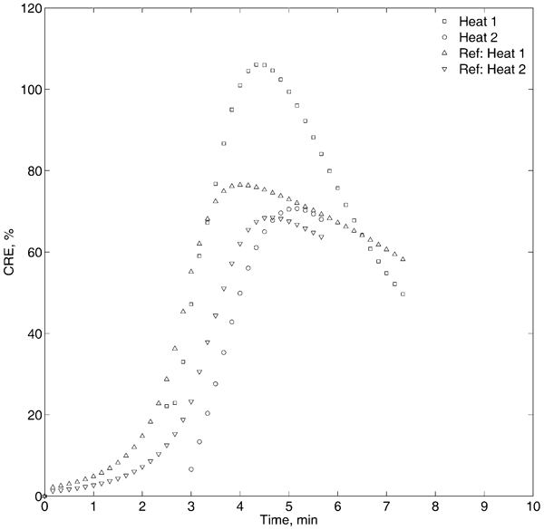
The mass ratio between the CO/(CO+CO₂) variation over time is seen in Fig. 6. The comparison between the predicted heats by the authors’ model shows a similar trend of decrease over time. There is a minor deviation for heat 1 in the very beginning, as the ratio increases more than for the other heats. Moreover, the CO₂ is predicted to increase up to a value of 1% of the carbon–oxygen gas.

Figure 6.

CO/(CO+CO₂) ratio plotted over time as predicted by model

Parameter study

The influence of a changed starting temperature on the decarburisation was investigated using heat 2 as the reference heat. This heat was chosen mainly because of the lower end temperature; thus, it allows for a vertical increase in the temperature profile without overshooting the end temperature to a value that is unreasonably high.

The average carbon concentration in the melt is plotted against time in Fig. 7. Here, it is seen that the decreasing mirrored ‘s’-like shape is consistent for all the cases. Moreover, it can be seen that an increased starting temperature results in a slightly lower carbon concentration. More specifically, for a temperature difference of 40°, the end concentration of carbon is predicted to differ up to 0·06 wt-% units.

Figure 7.

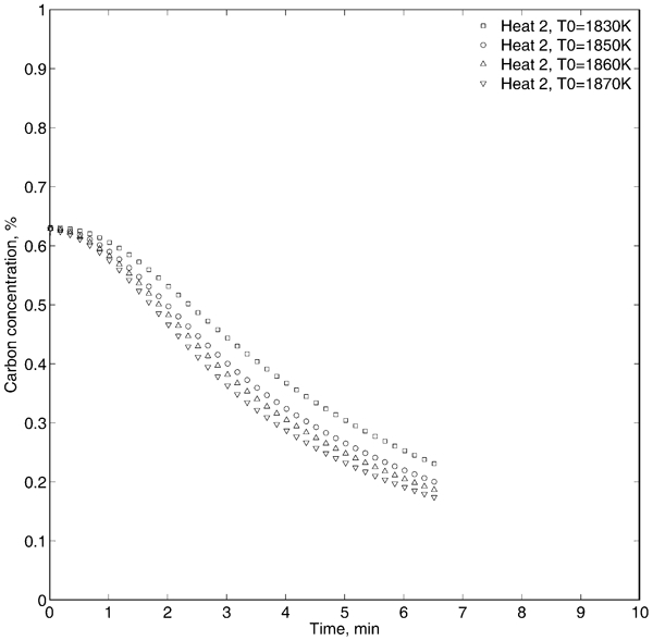
Carbon concentration as mass percentage plotted over time as predicted by model for different starting temperatures

In Fig. 8, the CRE value is plotted for different starting temperatures of the reference heat 2. Here, it can be noted that the trend for a higher starting temperature is a steeper increase in the CRE value and a narrower maximum than for lower starting temperatures. After the maximum value is reached, the decrease is more rapid for the high starting temperatures, intersecting the lower starting temperatures ∼3·5 min.

Figure 8.

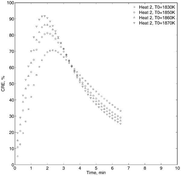
Carbon removal efficiency plotted over time as predicted by model for different starting temperatures

The CO/(CO+CO₂) gas mass ratio for different starting temperatures can be seen in Fig. 9. For 1830 and 1850 K, the decrease is smooth, and even and for the slightly higher temperatures, a saddle point is visible at ∼3 min. Moreover, a vague trend seen is that a higher starting temperature will give a slightly higher ratio of CO₂ towards the end of the first injection step. More specifically, the ratio decreases from almost 99·1% down to 98·1% for the highest temperature value.

Figure 9.

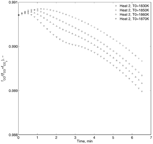
CO/(CO+CO₂) ratio plotted over time as predicted by model for different starting temperatures

The dissolved oxygen can be compared for the different starting temperature cases (Fig. 10). The overall variation over time is quite similar with increasing values, but with different slopes for the different cases. The main trend shows that a higher temperature dissolves more oxygen in the steel melt, which is expected from basic thermodynamics. More specifically, towards the end, a difference of 40° yields a difference of almost 150 ppm dissolved oxygen.

Figure 10.

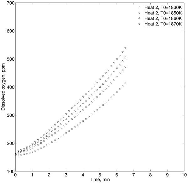
Dissolved oxygen concentration as mass parts per million plotted over time as predicted by model for different starting temperatures

Discussion

The choice of assuming an ideal dissolution of additions in the beginning was to isolate the temperature as a parameter. The dissolution is believed by the authors to have local effects around the cold charged addition lumps, which will locally affect the reactions for a region and during a period of time. Thus, to avoid unnecessary disturbances in the out phasing of the initial conditions, these assumptions were made.

The data for the reference heat 1 and the predicted heat in the author’s model agree rather well as seen in Figs. 4 and 5. However, the data in reference heat 2 deviates more from the model predictions. This can be due to the time translation and the temperature difference obtained as a consequence of that. The authors’ model does not consider Si; therefore, the model will poorly describe the initial state of the process. However, the aim of this study was to investigate the temperature influence on decarburisation in the model. Moreover, this will be of great help to interpret results when solving the energy equation in the future. It should be noted that the predicted CRE value for heat 1 goes >100% for a short period. This is due to the fact that, with the initial values used, the dissolved oxygen content decreases for some time, which corresponds to an extra amount of oxygen.

Details of the reaction products in the gas were earlier studied by Järvinen et al. 33 for a single bubble. However, the present approach is the first model to have the resolution needed to obtain these kinds of results for the whole converter and so could be used to compare different reaction model approaches in the future. In addition, it should be noted that these values may differ from gas concentrations measured only at the surface. More specifically, the gas in the lower parts of the converter may react further as it rises in the bath before exiting at the surface. Thus, the concentrations may change further.

From the results in Figs. 7 and 8, the temperature seems to correlate to the carbon concentration after a certain time in a linear fashion. Furthermore, a higher starting temperature seems to give a higher and narrower CRE maximum value. Moreover, the decarburisation seems to meet a thermodynamic limitation, which prevents it to continue the removal of carbon at a high efficiency. This is readily visible in Fig. 7, where the carbon limit is translated vertically depending on the temperature of the heat. Taking this into consideration, a suggestion can intuitively be made to always start decarburisation at a higher temperature in order to avoid cooling scrap additions that will increase the process time and lower the productivity. However, in a wider perspective, the temperature later in the process needs to be considered, i.e. a too high temperature must be prevented. Thus, depending on the carbon concentration after charging the necessary additions, this change may or may not be applicable. Moreover, the starting temperature of the AOD is a result of the tapping temperature of the electric arc furnace. Therefore, increased tapping temperatures in the electric arc furnace may increase costs further.

The results in Fig. 9 indicate that the decrease with time in CO in relation to CO₂ is stronger at higher temperatures. Furthermore, taking the results in Fig. 6 into account, the shape change of the curve seen for reference heat 1 is consistent with the shape seen for the highest starting temperature in the parameter study. The one thing these two cases have in common is a high pointy CRE maximum value, which may be the reason for this shape. More specifically, the highest temperature case shows a limit to the CO/(CO+CO₂) mass ratio at roughly 2·5 min. Initially, the trend is a relative rapid decrease up until 2·5 min. Thereafter, a slower decrease is apparent. This point seems to be connected to the CRE maximum, but this need to be explored in more detail in the future.

In Fig. 10, it was observed that the dissolved oxygen content in steel increased with an increased temperature. When the temperature is increased, the saturation limit is also increased. Therefore, the model predicts an increased dissolution of oxygen at higher process temperatures.

Conclusions

A study of the effect of the starting temperature on the decarburisation in an industrial AOD converter equipped with six tuyeres has been carried out using mathematical modelling coupled with a thermodynamic database. The flow field was obtained from a precalculated solution valid for an industrial AOD converter. In this study, the transport equations for different elements and reaction products were also solved to calculate the decarburisation. The influence of the starting temperature on the decarburisation was validated, and the effect on decarburisation was studied. Overall, the results show trends on how the isolated temperature affects the decarburisation. The main findings can be summarised as follows.

1. A higher temperature vertically translates the bulk carbon concentration after reaching thermodynamic limitations.

2. A higher starting temperature increases the CRE value more rapidly during the initial decarburisation stage under the assumptions made for this study.

3. The mass ratio between CO and CO₂ seems to show a limiting point of decrease. This should be studied in more detail in the future by allowing for local temperature variations.

The above described approach is seen as a first important step of a more thorough understanding of the temperature influence on decarburisation. Thus, it is planned that the fundamental model of the AOD process should be expanded to also include the solution of the energy equation, thereby allowing for local temperature variations.

Footnotes

Acknowledgements

The authors would like to thank Mr G. Lindstrand at Outokumpu Stainless for fruitful discussions regarding the process.

References

Fruehan

: ‘Reaction model for the AOD process’, Ironmaking Steelmaking, 1976, 3, (3), 153–158.

DebRoy

Robertson

DGC

: ‘Mathematical model for stainless steelmaking. 1: argon–oxygen and argon–oxygen–steam mixtures’, Ironmaking Steelmaking, 1978, 5, (5), 198–206.

DebRoy

Robertson

DGC

Leach

JCC

: ‘Mathematical model for stainless steelmaking: 2: application to AOD heats’, Ironmaking Steelmaking, 1978, 5, (5), 207–210.

Wei

J.-H

Zhu

D.-P

: ‘Mathematical modeling of the argon–oxygen decarburization refining process of stainless steel: Part I. Mathematical model of the process’, Metall. Mater. Trans. B, 2002, 33B, (1), 111–119.

Zhu

Wei

Shi

Shu

Jiang

Chi

: ‘Preliminary investigation of mathematical modeling of stainless steelmaking in an AOD converter: mathematical model of the process’, Steel Res. Int., 2007, 78, (4), 305–310.

Wei

J.-H

Cao

Zhu

H.-L

Chi

: ‘Mathematical modeling study on combined side and top blowing AOD refining process of stainless steel’, ISIJ Int., 2011, 51, (3), 365–374.

Järvinen

Pisilä

Kärnä

Ikäheimonen

Kupari

Fabritius

: ‘Fundamental mathematical model for AOD process. Part I: derivation of the model’, Steel Res. Int., 2011, 82, (6), 638–649.

Pisilä

Jarvinen

Karna

Ikaheimonen

Fabritius

Kupari

: ‘Fundamental mathematical model for AOD process. Part II: model validation’, Steel Res. Int., 2011, 82, (6), 650–657.

Tilliander

Jonsson

LTI

Jönsson

: ‘A three-dimensional three-phase model of gas injection in AOD converters’, Report no. 978-91-7501-266-7, KTH Royal Institute of Technology, Stockholm, Sweden, 2012.

10.

Andersson

NÅI

Tilliander

Jonsson

LTI

Jönsson

: ‘Fundamental decarburisation model of AOD process’, Ironmaking Steelmaking, 2012, DOI: 10.1179/1743281212Y.0000000060.

11.

Ternstedt

Gyllenram

Bengtsson

Jönsson

: ‘Using an AOD simulator workbench to support process control development’, Proc. 4th Int. Conf. on ‘Modelling and simulation of metallurgical processes in steelmaking’, Düsseldorf, Germany, 2011, METEC.

12.

Sjöberg

: ‘Some aspects on the scrap based production of stainless steel’, PhD thesis, KTH Royal Institute of Technology, Stockholm, Sweden, 1994.

13.

Andersson

NÅI

Tilliander

Jonsson

LTI

Jönsson

: ‘An in-depth model-based analysis of decarburization in the AOD process’, Steel Res. Int., 2012, 83, (11), 1039–1052.

14.

PHOENICS : ‘The PHOENICS-VR reference guide’, CHAM technical report no. 326, CHAM, London, UK, 2008.

15.

Spalding

: ‘IPSA 1981: new developments and computed results’, CFDU report no. HTS/81/2, Imperial College, London, UK, 1981.

16.

Tilliander

Jonsson

TLI

Jönsson

: ‘Fundamental mathematical modeling of gas injection in AOD converters’, ISIJ Int., 2004, 44, (2), 326–333.

17.

Jonsson

Grip

C.-E

Johansson

Jönsson

: ‘Three-phase (steel, slag, gas) modelling of the CAS-OB process’, AIME, Proc. 80th Steelmaking Conf., Chicago, IL, USA, 1997, 69–82.

18.

Jonsson

Jönsson

: ‘Modeling of fluid flow conditions around the slag/metal interface in a gas-stirred ladle’, ISIJ Int., 1996, 36, (9), 1127–1134.

19.

Solhed

Jonsson

Jönsson

: ‘A theoretical and experimental study of continuous-casting tundishes focusing on slag-steel interaction’, Metall. Mater. Trans. B, 2002, 33B, (2), 173–185.

20.

Zuber

Findlay

: ‘Average volumetric concentration in two-phase flow systems’, J. Heat Transfer, 1965, 453–468.

21.

Hibiki

Ishii

: ‘Development of one-group interfacial area transport equation in bubbly flow systems’, Int. J. Heat Mass Transfer, 2002, 45, (11), 2351–2372.

22.

Ishii

: ‘Drift flux model and derivation of kinematic constitutive laws’, NATO Advanced Study Institute, Hemisphere ed, 1977.

23.

Wallis

: ‘One-dimensional two-phase flow’; 1969, New-York, McGraw-Hill.

24.

Oeters

: ‘Metallurgy of steelmaking’; 1994, Düsseldorf, Verlag Stahleisen GmbH.

25.

Andersson

NÅI

Tilliander

Jonsson

LTI

Jönsson

: ‘Investigating the effect of slag on decarburization in an AOD converter using a fundamental model’, Steel Res. Int., 2012, DOI: 10.1002/srin.201200143.

26.

Reichel

Szekely

: ‘Mathematical models and experimental verification in the decarburization of industrial scale stainless steel melts’, Ironmaking Steelmaking, 1995, 22, (5), 41–48.

27.

Wei

J.-H

Zhu

D.-P

: ‘Mathematical modeling of the argon–oxygen decarburization refining process of stainless steel. Part II: application of the model to industrial practice’, Metall. Mater. Trans. B, 2002, 33B, (1), 121–127.

28.

Shi

Wei

Zhu

Shu

Jiang

Chi

: ‘Preliminary investigation of mathematical modeling of stainless steelmaking in an AOD converter: application of the model and results’, Steel Res. Int., 2007, 78, (4), 311–317.

29.

Andersson

Helander

Höglund

Shi

Sundman

: ‘Thermo-Calc & DICTRA, computational tools for materials science’, Calphad, 2002, 26, (2), 273–312.

30.

‘TCS metal slag interaction database, Version 3.0’, TCMSI1, Thermo-Calc Software AB, Stockholm, Sweden.

31.

‘SGTE substances database, Version 4.1’, SSUB4, Scientific Group Thermodata Europe, Saint Martin d’Hères, France.

32.

‘Resource-saving operation of stainless steel refining in VOD and AOD process’, RFCS project no. RFSR-CT-2007-00007, 2007–2010.

33.

Järvinen

Kärnä

Fabritius

: ‘A detailed single bubble reaction sub-model for AOD process’, Steel Res. Int., 2009, 80, (6), 429–436.