Calculation for grain growth rate of carbon steels by solute drag model considering segregation effect of each substitutional element

Abstract

Based on the solute drag model, a practical model incorporating the segregation effect is proposed to calculate grain growth rates in carbon steels. The segregation effect is modelled using two factors: the difference in atomic diameter between a solvent and a substitutional element, and the solubility of a substitutional element. By including the segregation energy, the proposed model enables the simulated retardation of grain growth by the addition of microalloying elements. The calculated grain growth rate by the proposed model shows reasonable correspondence between grain growth rates for experimental and calculated results. The temperature dependence of the grain growth rate is also well simulated.

Keywords

Solute drag Segregation Grain boundary Modelling Alloying element

Introduction

In order to produce high quality industrial parts made of metallic alloys, controlling the grain size by recrystallisation and grain growth is an effective method. For control of the grain size, process conditions are typically determined using equation (1). Here, is the mean grain size, and is the mean initial grain size. The parameters K and n in equation (1) are determined experimentally. Therefore, the grain size predicted by equation (1) is usually reliable for the corresponding experimental conditions. However, if the conditions used, such as temperature and chemical composition, are outside this range, the reliability of equation (1) becomes lower (1) There is another method to predict the grain growth rate. This is not an experimental method as above, but rather is a method constructed theoretically. It is well known that when a grain boundary moves during grain growth, the solution contained within the grain boundary is dragged. This phenomenon is called solute drag. Various models incorporating mathematical descriptions for solute drag have been proposed and subsequently improved by several authors.1^–5 With these models, the concentration profiles across grain boundaries or phase interfaces can be calculated. The velocity of boundary movement during phase transformation and recrystallisation were calculated by computing the balancing between dissipation energy and the driving force for solute drag.6^–9

In the solute drag model, the grain boundary property4 is defined for expressing the difference in properties between the interior of the grain and the grain boundary. It is difficult to measure the grain boundary property for calculating the velocity of grain boundary movement. However, the difference in properties needs to be defined to simulate the solute drag effect and the interaction between the solute and grain boundary more realistically.10 The interaction between the solute and the grain boundary is one of the causes of grain boundary segregation, especially in the case of microalloyed steels. Microalloyed Nb, V and Ti have a strong tendency to segregate at a grain boundary. These segregated elements retard boundary movement significantly in spite of low concentrations, even if the segregated elements do not form precipitates. For this reason, the segregation effect must be incorporated into the solute drag model. As far as we know, only a few studies have considered the segregation effect in the solute drag model based on experimental results. However, Nb was the only alloying element considered in these studies. 7 7,9

The purpose of the present study was to develop a practical model for calculating the grain growth rate including the influence of alloying elements and temperature. By coupling with thermodynamic calculations, the solute drag model can be applied to a wide range of alloying elements. Therefore, the solute drag model was chosen for the present study. A model that incorporates the segregation effect and the procedure to determine the segregation energy for each substitutional element is first proposed, based on the solute drag model. Next, using this model, the concentration profile across a grain boundary affected by the segregation effect of microalloying elements is calculated. Then, the influence of solute drag into grain size evolution is discussed. Finally, in order to show the validity of the model, the temperature dependence of grain growth rate is calculated, and the results are compared with experimental results.

Modelling

Calculation of concentration profile across grain boundary

Odqvist et al. developed the model to calculate the deviation from local equilibrium at moving phase interfaces in multicomponent systems. The method is based on finite interface mobility and solute drag theory.5 According to the solute drag model,5 the concentration profile across a grain boundary during grain growth can be calculated by coupling equations (2) and (3) (2) (3) Equations (2) and (3) represent fluxes of composition k under steady state conditions of grain growth rate v and the diffusion flux of composition k respectively. By solving the simultaneous equations (2) and (3), the concentration profile across a grain boundary at a grain growth rate v can be computed. α is the growing grain, and V_m is the molar volume per substitutional atom. The u fraction u_k is defined from the normal mole fraction x_k as (4) where l in the denominator is substitutional atoms only. Therefore, if there are no interstitial elements, the u fractions would be identical to the mole fractions. ∂φ_j is the gradient in diffusion potential, which works as the driving force for diffusion. The diffusion potential is defined as φ_j = μ_j−μ_n, where j is a substitutional solute and n is the solvent in a dilute solution. The parameters are related to the diffusion mobilities of different elements. (5) where δ_ij is the Kronecker delta with δ_ij = 0 unless i = j. If the atom is a substitutional element, a_j = 1. On the other hand, if the atom is an interstitial element, a = 0. M_j is the intrinsic diffusional mobility of species j.

Balancing driving force and dissipation energy for grain growth

The balance between the driving force and dissipation energy yields equation (6) (6) For calculating the grain growth rate, the driving force ΔG^tot is the excess energy that a polycrystal possesses over the energy of a single crystal. This excess energy is recognised as surface tension, explained by the Gibbs–Thomson effect. 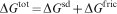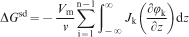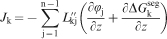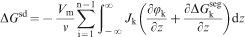Therefore, the driving force is defined by equation (7)11 (7) where σ is the grain boundary energy and is the mean radius of the grains. Total dissipation energy is energy resulting from the solute drag ΔG^sd in addition to dissipation of the Gibbs energy resulting from grain boundary friction ΔG^fric. The two kinds of dissipation energy are defined by equations (8) and (9) respectively5 (8) (9) where M is the boundary mobility of a pure metal (not the intrinsic diffusional mobility M_j). The grain growth rate at equilibrium between the driving force and total dissipation is the steady state velocity of grain growth v.

In order to calculate grain size evolution, the following procedure should be applied. Dissipation energy of the solute drag is caused by grain boundary movement with velocity v. If the grain boundary does not move, energy is not dissipated by the solute drag. The velocity v is solved by equation (6) at first time increment. During grain growth with velocity v, it is natural that grain size increases gradually. As a result of this, the driving force for grain growth decreases. Therefore, a grain size in equation (7) must be renewed, and then the velocity must be solved for the following time increment. This calculation flow corresponds to the suggestion5 as ‘The net driving force is obtained after subtracting the capillarity effect if the interface is curved’.

Grain boundary modelling for segregation effect

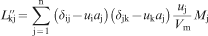
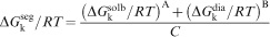
Some elements, especially microalloying elements, segregate at grain boundaries, and this significantly retards grain growth. Therefore, in order to calculate the grain growth rate, this segregation effect should be considered. According to a model by Hillert and Sundman4 for an interface during phase transformation, an energy gap across the boundary is defined to make the model more realistic. In the present study, a similar approach is applied to consider the segregation effect for the solute drag model. The segregation effect is introduced as segregation energy into the energy gap between the grain boundary and internal grain. The corresponding equations (3) and (8) are modified to equations (3)′ and (8)′ (3)′ (8)′ where expresses the segregation energy of composition k. It should be noted that is non-dimentionalised by dividing RT as well as φ_k.

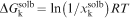
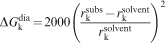
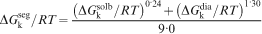
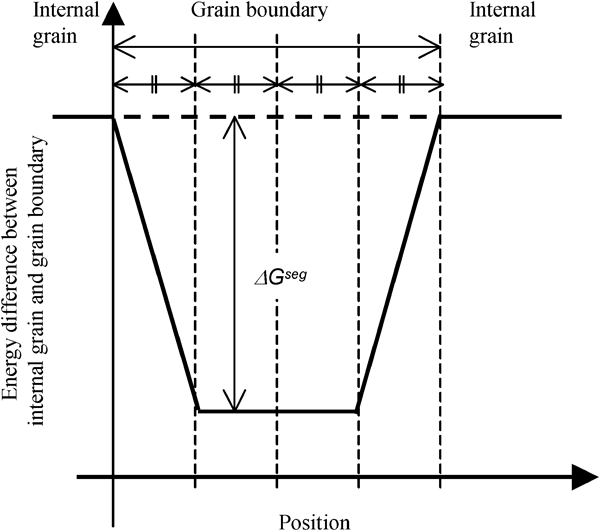
It is known that both the difference in atomic diameter between a solvent and a substitutional element and the solubility of a substitutional element strongly influence the segregation energy. 11 11,12 In order to consider both factors in ΔG^seg, it is assumed to be expressed as equation (10) (10) where ΔG^solb is the factor for the solubility and ΔG^dia is the factor for the difference in atomic diameter. A, B and C are parameters to be determined. Based on experimental results,11 ΔG^solb can be written as (11) By fitting experimental results,12 ΔG^dia derived from the difference in atomistic diameter between the radius of the substitutional element r^subs and the radius of the solvent r^solvent is related by (12) A grain boundary is divided into three zones. The central zone has an energy gap ΔG^seg from the interior of the grains. The properties of both side zones represent a gradual change between the interior of the grain and the central zone. A schematic diagram of this grain boundary model is shown in Fig. 1.

Figure 1

Schematic diagram of grain boundary model

Estimation of contribution rate of solute drag for grain growth

In the proposed model, the velocity of grain boundary movement is calculated by the balance of the driving force and dissipation energy of the solute drag and boundary friction. In this section, contribution rate of the solute drag for grain growth in total dissipation energy is discussed.

In order to estimate the driving force, an average grain size is assumed as 50 μm. For the boundary mobility of a pure metal, estimation by Turnbull13 is applied (13) where δ is the grain boundary width, D_gb is the grain boundary self-diffusion coefficient and b is the magnitude of the Burgers vector. According to equation (6), dissipation energy of the solute drag is estimated by ΔG^sd = ΔG^tot−ΔG^fric. Contribution rate of the solute drag and boundary friction is shown in Fig. 2. In this figure, it is obvious that the major contribution for grain growth is the solute drag in the range of the velocity of grain growth. Therefore, it is important that estimation of dissipation energy of the solute drag be exact to calculate grain growth rate.

Figure 2

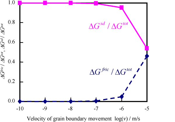
Contribution rate of solute drag and boundary friction for grain growth

Results and discussion

Parameters determination

There are three unknown parameters (A, B and C) in equation (10). The process to determine those parameters is discussed here. If there are three simultaneous equations for three unknown parameters, the equations can be solved to determine the parameters. This is the basic concept for determining parameters A, B and C.

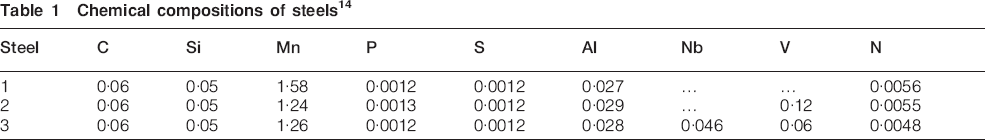
The grain growth rates under high temperature in five steels were measured.14 Grain growth rates measured in three steels without precipitations are applied for the present paper. The chemical compositions of the steels investigated are shown in Table 1. The three materials represent a base steel without microalloying elements (steel 1), a V alloyed steel (steel 2) and an Nb and V alloyed steel (steel 3). Squared grain diameters measured were proportional to time, and the factors of proportionality were defined as rate constant. Substituting the rate constants in these three steels at 1473 K into equation (6), three simultaneous equations for parameters A, B and C can be prepared. By solving those equations numerically, parameters A, B and C were determined. 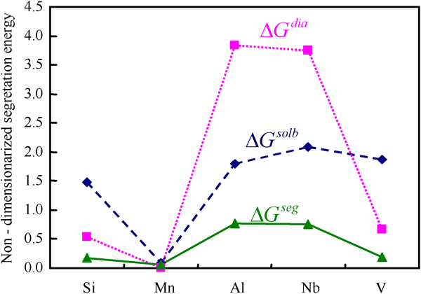With this procedure for determining the parameters, the segregation energy is expressed by equation (14) (14) The segregation energies of several elements determined by equation (14) at 1473 K are shown in Fig. 3. The energy derived from the difference in atomistic diameters between a solvent and a substitutional element, and the energy derived from the solubility of a substitutional element are also shown in Fig. 2. The values of 0·7 and 1·4 for the boundary energy were used by Hillert and Sundman4 and Enomoto6 respectively (concerning the value of 1·4, 8 kJ mol⁻¹ was used originally in Ref. 6). In Fig. 2, to non-dimensionalise the value for the y axis, the value of 1·4 is divided by RT. The values determined by equation (14) are not very different from these values. Therefore, the values determined by equation (14) are presumably valid.

Figure 3

Determined segregation energy of elements

Table 1

Chemical compositions of steels14

Steel	C	Si	Mn	P	S	Al	Nb	V	N
1	0·06	0·05	1·58	0·0012	0·0012	0·027	…	…	0·0056
2	0·06	0·05	1·24	0·0013	0·0012	0·029	…	0·12	0·0055
3	0·06	0·05	1·26	0·0012	0·0012	0·028	0·046	0·06	0·0048

Calculation conditions

The calculation procedure was coded using the Fortran programming language. The concentration profile across a grain boundary was solved with the forward difference method. It is known that the grain boundary energy σ changes depending on the kinds of alloying elements and their quantity. However, the grain boundary energy is defined as 0·2 J m⁻¹ for all steels since all influence of alloying elements are considered in equation (14) of the present study. The width of the grain boundary was defined as 10⁻⁹ m, and the calculation length was defined as three times the width of the grain boundary. The total number of grid points for a calculation was 601. The diffusion flux φ in each grid was calculated using Thermo-Calc verion S (Ref. 15) software along with the thermodynamic database TCFE6. Thermo-Calc is based on the minimisation of the total Gibbs energy of the system and on the CALPHAD approach.16^–18 The Fortran program was compiled with the Thermodynamic Calculation Interface to connect to Thermo-Calc.

Changing of concentration profile and grain size evolution

The concentration profile across a grain boundary was calculated for steel 3, which contains Nb and V, with and without consideration of segregation energy. The following calculation conditions were used: grain growth rate of 1·0×10⁻⁸ m s⁻¹ and temperature of 1473 K. The segregation energy for each element was determined by equation (14) and applied for the calculation considering the segregation energy. In the case of the calculation without consideration of the segregation energy, the value determined for Mn by equation (14) was defined as the segregation energy for all elements.

The calculated concentration profiles are shown in Fig. 4. In Fig. 4, y axis shows segregation of each element. u and u₀ are the u fraction within the grain boundary and the average concentration in bulk respectively. The x axis is normalised by the width of the grain boundary. The concentration profile calculated without consideration of the segregation energy shows a tendency for the element, which has a higher initial concentration, to have higher concentration at a grain boundary as well. On the other hand, the concentration of Nb increased significantly with consideration of the segregation energy. Figure 5 shows comparison of maximum segregation within grain boundary between the calculation with and without consideration of the segregation effect. It is recognisable that high magnitude of segregation by the calculation with consideration of the segregation effect is a cause of retardation of grain growth.

Figure 4

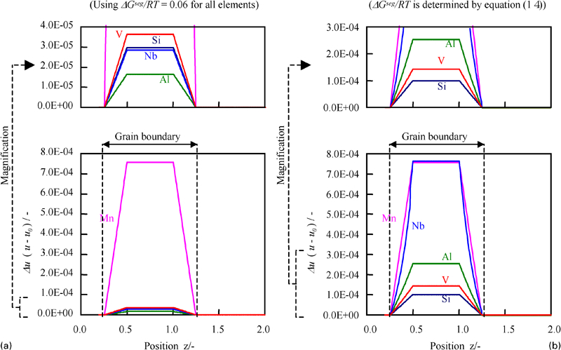
Calculated concentration profile across grain boundary of steel 3 (v = 1·0×10⁻⁸ m s⁻¹)

Figure 5

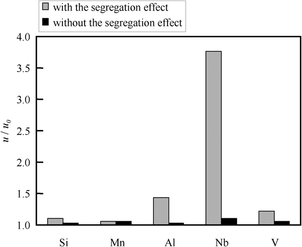
Comparison of maximum segregation within grain boundary of steel 3 between calculation with and without consideration of segregation effect

In the following, grain size evolution is calculated. The calculated grain diameter and driving force of steel 2 at 1473 K are shown in Fig. 6. In Fig. 7, the comparison of grain size evolution between experiment and calculations is shown. Three types of calculations are conducted: the proposed model, the model without considering the segregation effect of each substitutional element and the model considering only the boundary friction. Experiment and the only calculation by the proposed model show reasonable correspondence. It means that it is necessary when calculating grain growth rate to consider the solute drag and the segregation energy of each substitutional element.

Figure 6

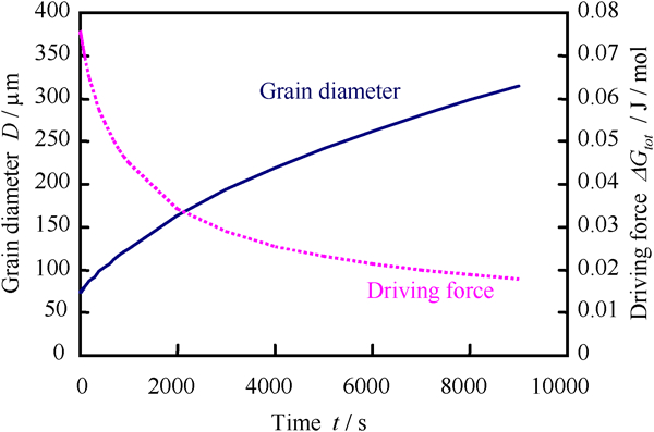
Change in grain diameter and driving force of steel 2

Figure 7

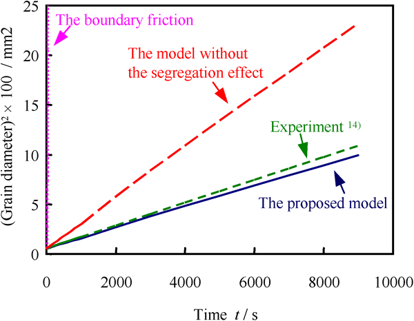
Comparison of grain growth of steel 2 between experiment and models

Calculation of temperature dependence of grain growth rate

The proposed model offers the possibility to simulate temperature dependence of the grain growth rate. This is because the diffusion potential φ, the solubility limit in ΔG^solb and the intrinsic diffusional mobilities of species M_j are included in the proposed model. All of these factors have temperature dependence. For the three materials in Table 1, the grain growth rates at 1423, 1473 and 1523 K are calculated by the proposed model. According to the experimental results,14 the initial grain size for the driving force is determined at each temperature. Equation (6) is a non-linear equation; therefore, the grain growth rate is solved by iterations. As mentioned above, squared grain diameter is proportional to time. Therefore, that relationship is described as (15) A comparison of the rate constant K is shown in Fig. 8. It is natural that the calculated results at 1473 K show reasonable correspondence, since the parameters in equation (14) were determined to fit the calculation results at 1473 K to the experimental results at 1473 K. On the other hand, the same parameters in equation (14) are given for the calculations at 1423 and 1523 K. The calculation results at 1423 and 1523 K simulate the influence of the microalloying elements and temperature well. These correspondences show the validity of the proposed model, which incorporates the segregation effect into the solute drag model, and its potential to predict the influence of alloying elements and temperature dependence.

Figure 8

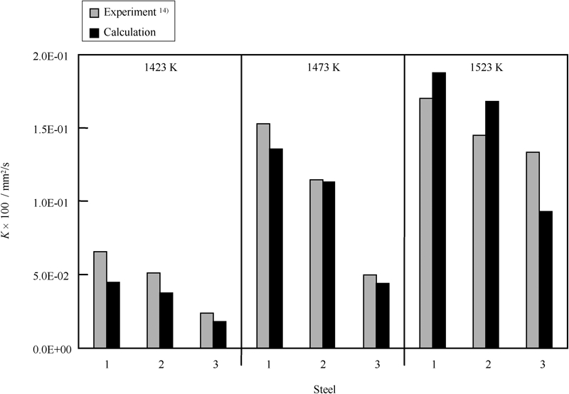
Comparison of grain boundary velocities between experiments and calculations

Summary

A practical model to calculate grain growth rate has been developed. This model is based on the solute drag model incorporating the segregation effect. Using this model, the concentration profiles across grain boundaries and grain size evolution were calculated. The calculated results to simulate the influence of microalloying elements and temperature for grain growth show reasonable agreement with experimental results.

References

Lucke

, Detert

: Acta Met. , 1957, 5, 628–637.

Cahn

: Acta Met. , 1962, 10, 789–798.

Lucke

, Stuwe

: ‘Recovery and recrystallisation’, 131; 1963, New York, Interscience Publications.

Hillert

, Sundman

: Acta Met. , 1976, 24, 731–743.

Odqvist

, Sundman

, Agren

: Acta Mater. , 2003, 51, 1035–1043.

Enomoto

: ISIJ Int. , 1999, 47, 3533–3540.

Suehiro

, Liu

, Agren

: Acta Mater. , 1996, 44, 4241–4251.

Suehiro

, Liu

, Agren

: Met. Mater. Trans. , 1998, 29A, 1029–1034.

Suehiro

: ISIJ Int. , 1998, 38, 547–552.

10.

Schalin

, Sundman

: TRITA-MAC-623, Royal Institute of Technology, Stockholm, Sweden: Solute Drag in Multicomponent Systems , 1999.

11.

‘Mikurososhiki-no-Netsurikigaku’, 135–145; 2005, Sendai, The Japan Institute of Metals.

12.

Nishizawa

: Mater. Jpn , 2001, 40, 437–441.

13.

Turnbull

: Trans. AIME , 1951, 191, 661–665.

14.

Kobayashi

: Tetsu-to-Hagane , 1977, 63, 73–79.

15.

Hillert

: in ‘Computer modeling of phase diagrams’, (ed. , Bennett

L H

, ed), 1–17; 1986, Warrendale, PA, TMS-AIME.

16.

Ågren

: Curr. Opin. Solid State Mater. Sci. , 1996, 1, 355–360.

17.

Sundman

: Scand. J. Metall. , 1991, 20, 79–85.

18.

Jansson

, Jönsson

, Sundman

, Ågren

: Thermochim. Acta , 1993, 214, 93–96.